A Simplified Algorithm for Inverting Higher Order Diffusion Tensors

Abstract

In Riemannian geometry, a distance function is determined by an inner product on the tangent space. In Riemann–Finsler geometry, this distance function can be determined by a norm. This gives more freedom on the form of the so-called indicatrix or the set of unit vectors. This has some interesting applications, e.g., in medical image analysis, especially in diffusion weighted imaging (DWI). An important application of DWI is in the inference of the local architecture of the tissue, typically consisting of thin elongated structures, such as axons or muscle fibers, by measuring the constrained diffusion of water within the tissue. From high angular resolution diffusion imaging (HARDI) data, one can estimate the diffusion orientation distribution function (dODF), which indicates the relative diffusivity in all directions and can be represented by a spherical polynomial. We express this dODF as an equivalent spherical monomial (higher order tensor) to directly generalize the (second order) diffusion tensor approach. To enable efficient computation of Riemann–Finslerian quantities on diffusion weighted (DW)-images, such as the metric/norm tensor, we present a simple and efficient algorithm to invert even order spherical monomials, which extends the familiar inversion of diffusion tensors, i.e., symmetric matrices.

1. Introduction

Diffusion tensor imaging is a technique based on nuclear magnetic resonance imaging, where one can non-invasively measure the orientation-dependent diffusivity of water molecules in human tissue, such as brain white matter [1,2]. As the behavior of water molecules inside tissue is influenced by the local geometry, this allows the indirect study of the structure and orientation of tissue. One of the goals in brain diffusion imaging is to use this information to trace the axonal fiber bundles that carry information between neurons in different parts of the brain. There are numerous models that relate the diffusion weighted imaging (DWI) signal to local physiological parameters [3]. One of the earlier models, and essentially the only one that is currently used in the clinical setting, is diffusion tensor imaging (DTI). In this model, one assumes anisotropic Gaussian diffusion.

By imaging the signal attenuation, first without an additional magnetic gradient and then comparing this with the signal when a directed magnetic field is applied, one can measure the so-called apparent diffusion coefficient (ADC) in each voxel. Measurements are repeated in several, e.g., 35 directions, and a second order model is fitted to describe this radially-symmetric diffusion profile. The diffusion length, typically measured at a scale of square micrometers per milliseconds, in direction $\mathbf{v}=(cos\varphi sin\theta ,sin\varphi sin\theta ,cos\theta )$, can be computed as:

$$D\left(\mathbf{v}\right)=\sum _{i,j=1}^3{\mathbf{D}}_{ij}{\mathbf{v}}_i{\mathbf{v}}_j$$

(1)

where ${\mathbf{D}}_{ij}$ is the element at the i-th row and j-th column of a $3\times 3$ matrix $\mathbf{D}$ (diffusion tensor) and ${\mathbf{v}}_i$ is the i-th component of vector $\mathbf{v}$.

Throughout this paper, the following notation is used: we express scalars with regular lower case fonts s (except for the diffusivity D), vectors with bold face lower cases $\mathbf{v}$ and tensors with bold face upper case fonts $\mathbf{T}$. Similar to the vectors, the components of the tensors are denoted with indices in the subscript ${\mathbf{T}}_{ij}$.

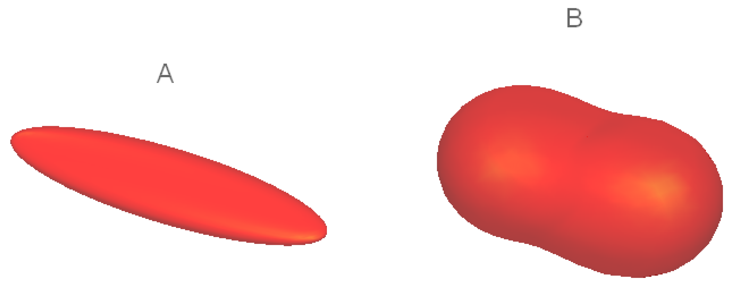
In the DTI case, two popular ways to visualize the diffusion profile is to either plot the set of points $\{\left(\mathbf{v}·{\mathbf{D}}^{\frac{1}{2}}·\mathbf{v}\right)·\mathbf{v}||\mathbf{v}|=1\}$, i.e., a glyph or $\{\mathbf{D}·\mathbf{v}|\left|\mathbf{v}\right|=1\}$, that is, an ellipsoid (see Figure 1). Note that in the D-induced metric, the vectors that constitute the ellipsoid have a unit length. The semi-axes of these ellipsoids are ${\lambda }_i{\mathbf{v}}_i$, where ${\lambda }_i$ are the eigenvalues and ${\mathbf{v}}_i$ the eigenvectors of the diffusion tensor.

Later, O’Donnell et al. connected the inverse of the diffusion tensor to a metric tensor [4,5]. Whereas the diffusion tensor tells how far a particle can diffuse in a given time, say a millisecond, a metric tensor tells how long the particle has to diffuse to reach, say, a micrometer distance from the starting point. Together with the assumption that fiber bundles coincide with the shortest curves relative to this metric, this interpretation of the diffusion tensor led to a fiber tracking algorithm, called geodesic tractography. Of course, given the complex architecture of the white matter, such an assumption is not always valid. Nevertheless, whenever axon tracking can be cast into a shortest path problem, efficient methods for extracting the geodesics become relevant and are valuable as such.

Figure 1. (A) The ellipsoid, i.e., the unit level set of the inverse of a diffusion tensor; and (B) the glyph determined by the same diffusion tensor.

Figure 1. (A) The ellipsoid, i.e., the unit level set of the inverse of a diffusion tensor; and (B) the glyph determined by the same diffusion tensor.

High resolution diffusion magnetic resonance imaging (HARDI) brought axon tracking to another level by scanning far more imaging directions than is necessary for DTI. The diffusion profiles (glyphs) could now have a more complex form than a symmetric peanut. The most obvious disadvantage of the DTI model is the fact that it works very well when a voxel only contains a single fiber bundle, but fails completely when there are two or more fiber populations with distinct orientations. A number of models have been suggested to overcome this, but none of them has the intuitive Riemannian interpretation as in DTI. In an effort to extend the Riemannian framework into HARDI, approaches employing Riemann–Finsler geometry were suggested [6,7,8,9,10]. The essential difference with respect to Riemannian geometry is that the distance function is determined by a position- and direction-dependent norm function instead of a position-dependent inner product. Axons that intersect each other in a single voxel, which were impossible to distinguish in the DTI setting, could now be resolved to some extent using the Riemann–Finsler geometry [6]. An algorithm extending the regular streamline tracking to the Finslerian framework, where the metric is determined by the Hessian of the local Finsler-norm, could apparently successfully extract crossing bundles of fibers in human brain, such as typical of corpus callosum, corona radiata and cingulum [8]. However, the approach in [8], while being a straightforward higher order generalization of DTI, has a shortcoming that we wish to remove.

The Finsler-norm function was computed as the (multiplicative) Möbius-inverse [11] of the diffusion profile, which is typically not a spherical tensor (monomial) itself.

We would like to treat diffusion and norm profiles on an equal footing, as is the case for the diffusion and metric tensor in the Riemannian framework [4,12]. This requires that the (higher order) diffusion and metric tensors can be related to each other via a unique inverse operation.

In this contribution, we describe a simple heuristic algorithm for computing the inverse of a higher order tensor. In Section 2, we briefly provide the motivation for our approach, although, in essence, equivalent to that of other authors [13,14], besides aesthetic, but also practical and efficient. In Section 3, we describe our simple inversion algorithm in detail, as well as by means of visual illustration and show some examples. We finish with conclusions in Section 5.

2. The Parsimony of Monomials

By a (spherical) monomial, we mean a function of the following type:

$$\sum _{i_1,\cdots ,i_n=1}^3{\mathbf{A}}_{i_1\cdots i_n}{\mathbf{v}}_{i_1}\cdots {\mathbf{v}}_{i_n}$$

(2)

where ${\mathbf{A}}_{i\cdots n}\in \mathbb{R}$, $\left|\mathbf{v}\right|=1$ and n is a fixed even positive number. This in contrast with a (spherical) polynomial:

$$\sum _{n=0,2,\cdots }\left(\sum _{i_1,\cdots ,i_n=1}^3{\mathbf{A}}_{i_1{i}_2\cdots i_n}{\mathbf{v}}_{i_1}\cdots {\mathbf{v}}_{i_n}\right)$$

(3)

In both cases, running through all unit vectors $\mathbf{v}$ on the two-sphere, one obtains a spherical surface homeomorphic to the two-sphere.

The general protocol of converting raw HARDI data to a diffusion profile (a spherical polynomial or an equivalent monomial) is described elsewhere [7,13,14], and we do not repeat it here. The number of directions along which the ADC can be measured and the resulting angular resolution is, in practice, limited. This implies that it makes no sense to use a very high order model to capture the diffusion profile [15]. Therefore, a spherical polynomial of order from 2 to 6 is typically sufficient to estimate the diffusion profiles. The conventional formula that translates the signal $S_D$ obtained with a diffusion-sensitized gradient to an “apparent diffusion coefficient” D is as follows:

$$D=\frac{ln(S_0/S_D)}{b}$$

(4)

Here, $S_0$ is the signal without diffusion weighting magnetic gradient and:

$$b={(\gamma G\Delta )}^2(\Delta -\delta /3)$$

(5)

where δ is the gradient pulse duration, Δ is the time between gradient pulses, γ is the gyromagnetic ratio and G is the magnitude of the magnetic gradient. In DWI, one cannot distinguish between the two possible directions (forward/backward) along a specified orientation. For this reason, at least in the conventional HARDI, the diffusion profile is always radially symmetric. As a consequence, any function describing such a profile is also radially symmetric.

For the reasons mentioned above, we model diffusion profiles with fourth order monomials fitted to the signal data as in [7,14]. It can be shown that a monomial expression is equivalent to spherical harmonics or a polynomial expression of equal order [7,16,17]. Therefore, why use monomials? One reason is that they are a compact expression that directly generalizes the DTI tensor concept. Another reason is that in exploiting the Riemann–Finsler concepts of norms and metric tensors, one computes from a position ($\mathbf{x}$) -dependent norm a position and direction (x, y) -dependent metric tensor by calculating the Hessian of the squared norm function with respect to $\mathbf{y}$ as follows:

$${\mathbf{G}}_{ij}(\mathbf{x},\mathbf{y})=\frac{1}{2}\frac{{\partial }^2{F}^2\left(x\right)}{\partial {\mathbf{y}}_i\partial {\mathbf{y}}_j}$$

(6)

where $\mathbf{G}$ is the metric tensor and F is the norm function. Indeed, monomials are extremely simple/fast to differentiate twice. The third reason is that, as we will show in the next section, an even order symmetric monomial can be inverted, so that the inverse is also (an equal order) monomial, and moreover, this inversion can be done in a simple setting of matrix multiplication.

The main motivation for computing these position- and orientation-dependent glyphs and (Finsler) metric tensors is that this gives a straightforward extension of DTI streamline tracking to HARDI, allowing the extraction of multiple fiber orientations in a single voxel.

3. Inversion of Even Order Fully-Symmetric Tensors

Brazell et al. [18] show how even order tensors can be inverted in the sense of the so-called Einstein contracted product. In our context, the tensors are totally symmetric, which allows some essential simplifications to the more general formulation of inversion in [18].

To keep the notation simple, we define the Einstein contracted product (ECP) only for fourth order tensors. For a general definition, see [18]. Let $\mathbf{A}$ and $\mathbf{B}$ be fourth order tensors. The ECP of these, $\mathbf{C}$, is a fourth order tensor with elements:

$${\mathbf{C}}_{ijkl}=\sum _{m,n=1}^3{\mathbf{A}}_{ijmn}·{\mathbf{B}}_{mnkl}$$

(7)

Recall that even order tensors can be regarded as nested matrices. In particular, a fourth order tensor can be denoted by a matrix of matrices. For example, a fourth order tensor $\mathbf{A}$ can be explicitly written down as follows:

$$\mathbf{A}=\left(\begin{array}{ccc}\left(\begin{array}{ccc}{\mathbf{A}}_{1111}& {\mathbf{A}}_{1112}& {\mathbf{A}}_{1113}\\ {\mathbf{A}}_{1121}& {\mathbf{A}}_{1122}& {\mathbf{A}}_{1123}\\ {\mathbf{A}}_{1131}& {\mathbf{A}}_{1132}& {\mathbf{A}}_{1133}\end{array}\right)& \left(\begin{array}{ccc}{\mathbf{A}}_{1211}& {\mathbf{A}}_{1212}& {\mathbf{A}}_{1213}\\ {\mathbf{A}}_{1221}& {\mathbf{A}}_{1222}& {\mathbf{A}}_{1223}\\ {\mathbf{A}}_{1231}& {\mathbf{A}}_{1232}& {\mathbf{A}}_{1233}\end{array}\right)& \left(\begin{array}{ccc}{\mathbf{A}}_{1311}& {\mathbf{A}}_{1312}& {\mathbf{A}}_{1313}\\ {\mathbf{A}}_{1321}& {\mathbf{A}}_{1322}& {\mathbf{A}}_{1323}\\ {\mathbf{A}}_{1331}& {\mathbf{A}}_{1332}& {\mathbf{A}}_{1333}\end{array}\right)\\ \left(\begin{array}{ccc}{\mathbf{A}}_{2111}& {\mathbf{A}}_{2112}& {\mathbf{A}}_{2113}\\ {\mathbf{A}}_{2121}& {\mathbf{A}}_{2122}& {\mathbf{A}}_{2123}\\ {\mathbf{A}}_{2131}& {\mathbf{A}}_{2132}& {\mathbf{A}}_{2133}\end{array}\right)& \left(\begin{array}{ccc}{\mathbf{A}}_{2211}& {\mathbf{A}}_{2212}& {\mathbf{A}}_{2213}\\ {\mathbf{A}}_{2221}& {\mathbf{A}}_{2222}& {\mathbf{A}}_{2223}\\ {\mathbf{A}}_{2231}& {\mathbf{A}}_{2232}& {\mathbf{A}}_{2233}\end{array}\right)& \left(\begin{array}{ccc}{\mathbf{A}}_{2311}& {\mathbf{A}}_{2312}& {\mathbf{A}}_{2313}\\ {\mathbf{A}}_{2321}& {\mathbf{A}}_{2322}& {\mathbf{A}}_{2323}\\ {\mathbf{A}}_{2331}& {\mathbf{A}}_{2332}& {\mathbf{A}}_{2333}\end{array}\right)\\ \left(\begin{array}{ccc}{\mathbf{A}}_{3111}& {\mathbf{A}}_{3112}& {\mathbf{A}}_{3113}\\ {\mathbf{A}}_{3121}& {\mathbf{A}}_{3122}& {\mathbf{A}}_{3123}\\ {\mathbf{A}}_{3131}& {\mathbf{A}}_{3132}& {\mathbf{A}}_{3133}\end{array}\right)& \left(\begin{array}{ccc}{\mathbf{A}}_{3211}& {\mathbf{A}}_{3212}& {\mathbf{A}}_{3213}\\ {\mathbf{A}}_{3221}& {\mathbf{A}}_{3222}& {\mathbf{A}}_{3223}\\ {\mathbf{A}}_{3231}& {\mathbf{A}}_{3232}& {\mathbf{A}}_{3233}\end{array}\right)& \left(\begin{array}{ccc}{\mathbf{A}}_{3311}& {\mathbf{A}}_{3312}& {\mathbf{A}}_{3313}\\ {\mathbf{A}}_{3321}& {\mathbf{A}}_{3322}& {\mathbf{A}}_{3323}\\ {\mathbf{A}}_{3331}& {\mathbf{A}}_{3332}& {\mathbf{A}}_{3333}\end{array}\right)\end{array}\right)$$

(8)

Further, recalling that in our case, the tensors are totally symmetric, we have, in particular, the following equivalence:

$${\mathbf{A}}_{ijkl}={\mathbf{A}}_{klij}$$

(9)

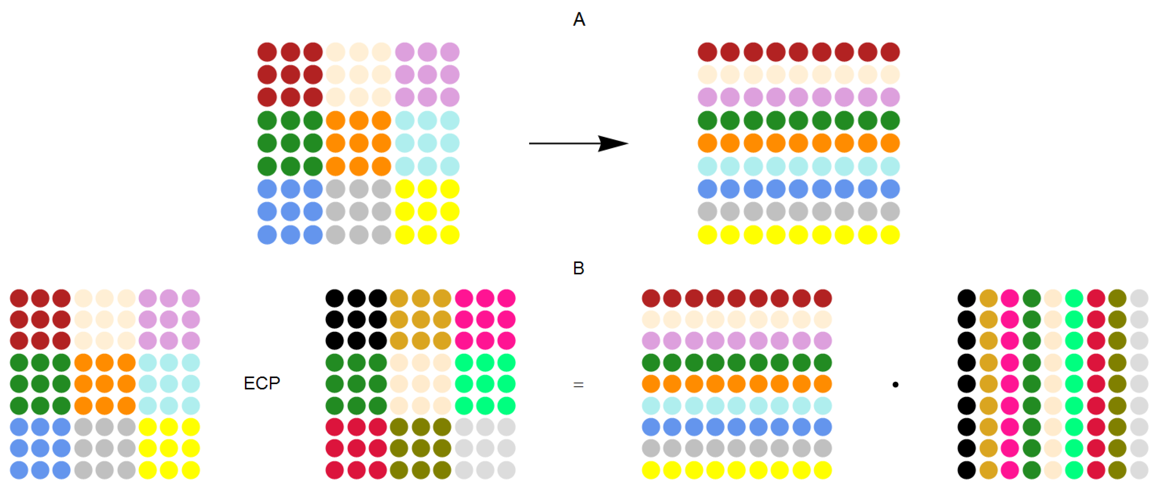
This means that the ECP of $\mathbf{A}$ and $\mathbf{B}$ can be seen as componentwise products of all “inner” matrices. Furthermore, if we “reshape” the inner matrices, ECP is actually a matrix product (see Figure 2).

Figure 2. (A) An illustration of how the nested matrix should be reshaped to replace the Einstein contracted product (ECP) with an ordinary matrix product; (B) the correspondence between ECP and the matrix dot product after manipulating the tensor shape.

Figure 2. (A) An illustration of how the nested matrix should be reshaped to replace the Einstein contracted product (ECP) with an ordinary matrix product; (B) the correspondence between ECP and the matrix dot product after manipulating the tensor shape.

To find the inverse tensor ${\mathbf{A}}^{-1}$ of $\mathbf{A}$, we need to solve this from the following equation:

$$sym\left(\sum _{m,n=1}^3{\mathbf{A}}_{ijmn}·{\mathbf{A}}_{mnkl}^{-1}\right)={\mathfrak{I}}_{ijkl}$$

(10)

where the left-hand side is the symmetrized ECP of $\mathbf{A}$ and ${\mathbf{A}}^{-1}$, and $\mathfrak{I}$ is the fourth order identity tensor. The fully symmetric identity tensor $\mathfrak{I}$ is defined as follows:

$${\mathfrak{I}}_{ijkl}=\frac{1}{3}\left({\delta }_{ik}{\delta }_{jl}+{\delta }_{il}{\delta }_{jk}+{\delta }_{ij}{\delta }_{kl}\right)$$

(11)

where:

$${\delta }_{ij}=\left\{\begin{array}{cc}1,\hfill & i=j\hfill \\ 0,\hfill & i\ne j\hfill \end{array}\right.$$

(12)

The symmetric identity tensor $\mathfrak{I}$ in matrix notation is then:

$$\left(\begin{array}{ccc}\left(\begin{array}{ccc}1& 0& 0\\ 0& \frac{1}{3}& 0\\ 0& 0& \frac{1}{3}\end{array}\right)& \left(\begin{array}{ccc}0& \frac{1}{3}& 0\\ \frac{1}{3}& 0& 0\\ 0& 0& 0\end{array}\right)& \left(\begin{array}{ccc}0& 0& \frac{1}{3}\\ 0& 0& 0\\ \frac{1}{3}& 0& 0\end{array}\right)\\ \left(\begin{array}{ccc}0& \frac{1}{3}& 0\\ \frac{1}{3}& 0& 0\\ 0& 0& 0\end{array}\right)& \left(\begin{array}{ccc}\frac{1}{3}& 0& 0\\ 0& 1& 0\\ 0& 0& \frac{1}{3}\end{array}\right)& \left(\begin{array}{ccc}0& 0& 0\\ 0& 0& \frac{1}{3}\\ 0& \frac{1}{3}& 0\end{array}\right)\\ \left(\begin{array}{ccc}0& 0& \frac{1}{3}\\ \frac{1}{3}& 0& 0\\ \frac{1}{3}& 0& 0\end{array}\right)& \left(\begin{array}{ccc}0& 0& 0\\ 0& 0& \frac{1}{3}\\ 0& \frac{1}{3}& 0\end{array}\right)& \left(\begin{array}{ccc}\frac{1}{3}& 0& 0\\ 0& \frac{1}{3}& 0\\ 0& 0& 1\end{array}\right)\end{array}\right)$$

(13)

This inversion clearly generalizes the matrix inversion used to convert the familiar second order diffusion tensor to a metric tensor. Due to the symmetries between the tensor elements, the inverse operation can be performed in the three simple steps of Algorithm 1.

Algorithm 1: Computing the inverse of a symmetric fourth order tensor $\mathbf{A}$.

1. Compute the Einstein product $\mathbf{P}$ of the chosen tensor $\mathbf{A}$ with a symmetric variable tensor $\mathbf{V}$,  with components $v_{1111},v_{1112},\cdots$, e.g., as a matrix product, as in Figure 2; 2. reshape the result to a four tensor and symmetrize with formula ${\mathbf{P}}_{ijkl}^{sym}=\frac{1}{4!}{\sum }_{\sigma \in S_4}{\mathbf{P}}_{\sigma \left(i\right)\sigma \left(j\right)}{\mathbf{I}}_{\sigma \left(k\right)\sigma \left(l\right)}$; 3. Solve the 15 equations ${\mathbf{P}}_{1111}^{sym}={\mathfrak{I}}_{1111},{\mathbf{P}}_{1112}^{sym}={\mathfrak{I}}_{1112},\cdots ,{\mathbf{P}}_{3333}^{sym}={\mathfrak{I}}_{3333}$.

Here, $S_4$ refers to the set of all permutations of a set of four elements. For a visually intuitive explanation on symmetrizing a fourth order tensor, see e.g., [7]. One should not directly solve the tensor with the matrix inverse, since the highly symmetric tensor in matrix form is singular. By solving only the 15 necessary equations, we avoid a system of over-determined equations and get reliable results, which are different from that obtained by the plain pseudo-inverse approach.

It is interesting to see that this also perfectly matches with the intuition of inverting the so-called glyph, which is the set:

$$\left\{\sum _{i,j,k,l=1}^3{\mathbf{A}}_{ijkl}{\mathbf{y}}_i{\mathbf{y}}_k{\mathbf{y}}_l||\mathbf{y}|=1\right\}$$

(14)

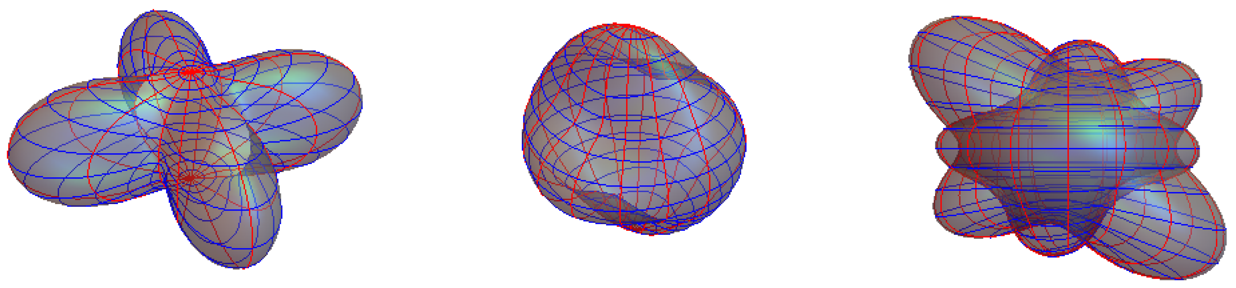
The glyph (and the unit level set) of $\mathfrak{I}$ is the unit two-sphere. For an illustration of dODF-based glyphs and their ECP-inverses, see Figure 3. Clearly, in the orientations that correspond to larger diffusivity, the ECP-inverse is small, just as the case with inverting the second order tensor. Using this inverted tensor, one can further compute Finslerian quantities, such as geodesics, that can be exploited, e.g., in the context of diffusion-based fiber tracking.

Figure 3. (Left) The glyph represents the diffusion orientation distribution function. (middle) The glyph represents the ECP-inverse of this; and (right) another tensor glyph with its inverse is plotted together. For visual comparison, lines of longitudes are indicated in red and latitudes in blue.

Figure 3. (Left) The glyph represents the diffusion orientation distribution function. (middle) The glyph represents the ECP-inverse of this; and (right) another tensor glyph with its inverse is plotted together. For visual comparison, lines of longitudes are indicated in red and latitudes in blue.

4. Applications in Fiber Tracking

Once a proper diffusion-induced metric has been defined for a DWI image, one may apply tractography in order to reconstruct the fibrous tissue structure of the underlying neural axons of the white matter. One prominent approach in deterministic tractography is to model the fibers as minimum length paths, i.e., the geodesics in the given metric space. The main assumption in this technique is that the fibers tend to follow the most efficient diffusion propagation, thereby corresponding to the paths of shortest distance [19,20]. A recently-introduced geodesic tractography technique obtains the pathways as solutions of Euler–Lagrange (EL) equations in Riemannian or Finslerian space [21,22]. This tractography approach can capture multi-valued geodesics connecting two given points or regions by considering the geodesics as a function of position and direction. A manifold is defined using as a metric the adjugate of the diffusion tensor or the inverted dODF. Please note that we use the dODF obtained by fitting the HARDI data with a procedure described by Descoteaux et al. [23]. By applying the inversion technique proposed here to the dODF-tensors and subsequently feeding them as input for the tractography, we have obtained some preliminary results. The tractography was done in a $10\times 10\times 30$ cube cut from the healthy human dataset obtained by a Philips scanner with resolution $2\times 2\times 2$ mm, b-value of 1000 s/mm${}^2$ and 128 gradient directions.

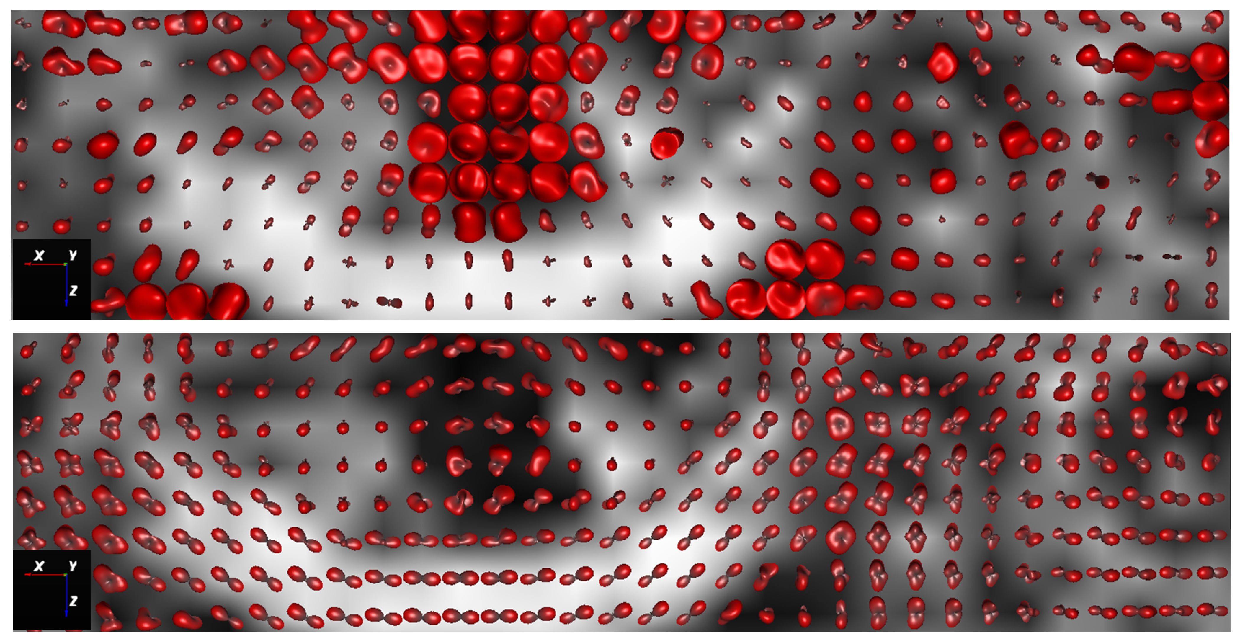
Given the region of interests, geodesics are computed from all discrete coordinates to a large number of directions until they meet one of the boundaries. To determine which of the numerous geodesics corresponds to the most likely fiber, we have used the line-plane intersection method, as in [22,24]. In this way, the geodesics are cut once they enter one of the user-defined regions of interest. Figure 4 indicates the ODFs and the inverted ODFs for a part of the centrum semiovale. In Figure 5, few fiber tracts for corpus callosum (CC) have been computed, and their corresponding ODFs and the inverted ODFs per fiber voxel have been indicated. 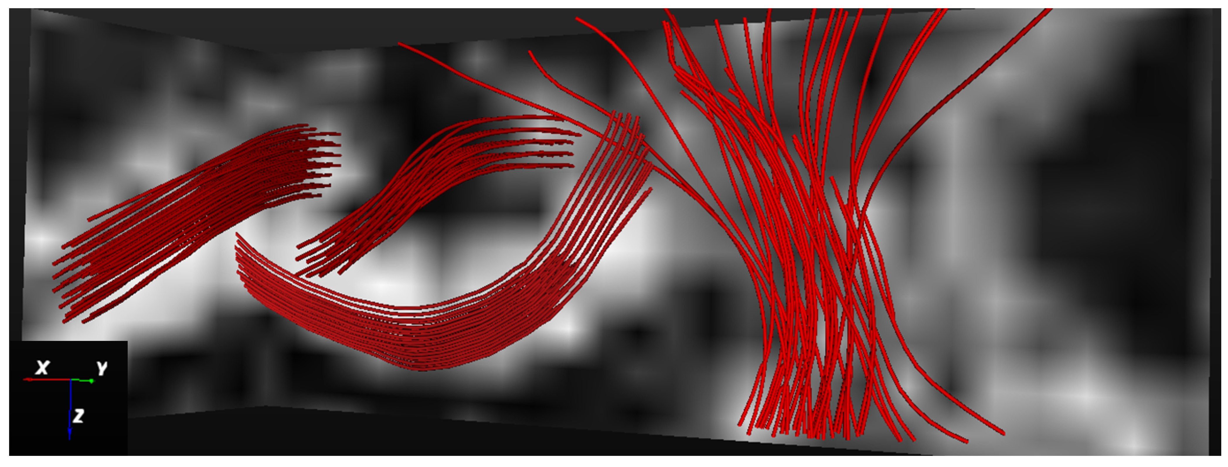Figure 6 shows the tractography result for the area of corona radiata (CR), CC and cingulum (CG).

Figure 4. Inverted fourth order orientation distribution function (ODF) field (top) and its corresponding ODF field (bottom) from part of the centrum semiovale.

Figure 4. Inverted fourth order orientation distribution function (ODF) field (top) and its corresponding ODF field (bottom) from part of the centrum semiovale.

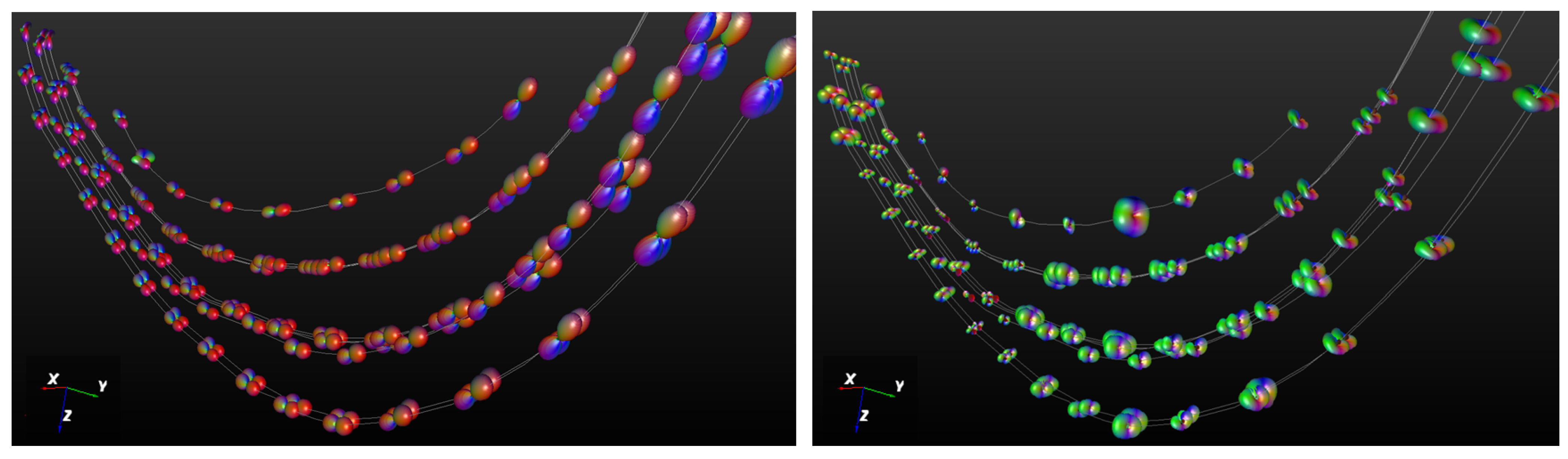
Figure 5. Corpus callosum fibers: (left) the corresponding ODFs per fiber voxel and (right) the corresponding inverted ODFs per fiber voxel.

Figure 5. Corpus callosum fibers: (left) the corresponding ODFs per fiber voxel and (right) the corresponding inverted ODFs per fiber voxel.

Figure 6. Fiber tracts for corpus callosum (CC), corona radiata (CR) and cingulum (CG).

Figure 6. Fiber tracts for corpus callosum (CC), corona radiata (CR) and cingulum (CG).

5. Conclusions

We have proposed to use a symmetrized contracted Einstein product in the inversion of higher even order tensors in the context of HRDW-image analysis. We have shown that this approach generalizes the approach of O’Donnell et al., which applies tools from Riemannian geometry in the DTI setting. The unit level set of the ECP-inverted monomial generalizes the metric ellipsoid used in the DTI-setting. By employing monomials in modeling the diffusion profiles, we obtain an intuitive and consistent framework for the analysis and tractography on DW-images. We also illustrated how this inversion can be efficiently computed using a simple Algorithm 1. This is useful, since, in the case a tensor is of high order, the computation of indexed sums can easily become time consuming.