
Operational Approach and Solutions of Hyperbolic Heat Conduction Equations

Faculty of Physics, Moscow State University, Leninskie Gory, Moscow 119991, Russia
Axioms 2016, 5(4), 28; https://doi.org/10.3390/axioms5040028
Submission received: 27 October 2016
/
Revised: 6 December 2016
/
Accepted: 6 December 2016
/
Published: 12 December 2016
(This article belongs to the Special Issue Special Functions: Fractional Calculus and the Pathway for Entropy Dedicated to Professor Dr. A.M. Mathai on the occasion of his 80th Birthday)
Abstract
:We studied physical problems related to heat transport and the corresponding differential equations, which describe a wider range of physical processes. The operational method was employed to construct particular solutions for them. Inverse differential operators and operational exponent as well as operational definitions and operational rules for generalized orthogonal polynomials were used together with integral transforms and special functions. Examples of an electric charge in a constant electric field passing under a potential barrier and of heat diffusion were compared and explored in two dimensions. Non-Fourier heat propagation models were studied and compared with each other and with Fourier heat transfer. Exact analytical solutions for the hyperbolic heat equation and for its extensions were explored. The exact analytical solution for the Guyer-Krumhansl type heat equation was derived. Using the latter, the heat surge propagation and relaxation was studied for the Guyer-Krumhansl heat transport model, for the Cattaneo and for the Fourier models. The comparison between them was drawn. Space-time propagation of a power–exponential function and of a periodic signal, obeying the Fourier law, the hyperbolic heat equation and its extended Guyer-Krumhansl form were studied by the operational technique. The role of various terms in the equations was explored and their influence on the solutions demonstrated. The accordance of the solutions with maximum principle is discussed. The application of our theoretical study for heat propagation in thin films is considered. The examples of the relaxation of the initial laser flash, the wide heat spot, and the harmonic function are considered and solved analytically.
1. Introduction
The differential equations (DE) are of paramount importance both in pure mathematics and in physics since they describe a very broad range of physical processes. Rapid development of computer methods and machine calculations in the 21st century facilitated equation solving. A good description of the major numerical methods is given, for example, in [1,2,3,4,5,6]. Here they allow numerical modelling of complicated physical processes [7,8,9,10,11,12,13,14,15,16,17,18,19], including multidimensional heat transfer in rectangles and cylinders [20,21,22,23]. However, proper understanding of the solutions and of the obtained results can be best done when they are obtained in analytical form. Analytical studies generally are more suitable for the analysis of the undergoing physical processes rather than numerical models, the latter giving precise description of the performance of the devices and of the specific studied cases. Analytical solutions are highly appreciated, but only a few types of DE allow explicit, if any, exact analytical solutions. Recently some fractional ordinary DE and partial differential equations (PDE) were analyzed and analytically solved in [24,25,26,27,28,29,30,31,32,33,34,35,36,37]. They benefit from the use of special functions [38,39,40]. The mathematical instruments, used to solve DE, generally range from a variety of integral transforms [41,42] to expansion in a series of generalized orthogonal polynomials [43] with many variables and indices [44,45,46], which arise naturally in studies of physical problems, such as the radiation and dynamics of beams of charges [47,48,49,50,51,52,53,54], heat and mass transfer [55,56,57,58,59], etc. Moreover, exponential operators and matrices are currently used also for description of such nature fundamentals as neutrino and quarks in theoretical [60,61,62,63,64,65] and in experimental [66,67,68] frameworks. The method of inverse differential and exponential operators has multiple applications for treating the above mentioned problems and related processes; some examples of DE solution by the inverse derivative method with regard to the heat equation, the diffusion equation, and their extensions, involving the Laguerre derivative, were given in [46,69,70,71,72,73]. Orthogonal polynomials can be defined in forms through operational relations [74], although we will also use their series presentations.
In what follows we treat the problem of heat conduction by the operational method in the framework of classical thermodynamics. We obtain, compare, and explore exact solutions for relevant DE in the framework of heat conduction models for Fourier [75], Cattaneo [76], and Guyer-Krumhansl [77] heat laws.
2. Fourier Heat Equation and Its Operational Solution
Fourier’s law of heat propagation imposes a linear relation between the temperature gradient and the heat flux. This is one of the most popular laws in continuum physics and it is in excellent agreement with everyday life and with more than 90% experiments. Recently the Fourier heat equation with a linear term
was studied operationally as a special case of the Schrödinger equation in imaginary time [70,73]. The solution of such DE with the initial condition is given by the Gauss transform:
where , , . The heat diffusion operator
was thoroughly explored by Srivastava in [78]. The exponential differential operator (3) reduces to the exponential differential operator upon the application of the following integral presentation [41]:
where in our case. Thus, the above formula reads as follows:
The action of the operator of translation for produces a shift
The solution (2) consists of the action of the evolution operator on the initial condition , which is transformed by and . Interestingly, for the Airy initial condition the operational method readily yields the fading oscillating solution without any spread [71], while the solution for the Gauss initial function demonstrates the spread of the packet.
In direct analogy with (1) the following two dimensional DE
with the initial condition has the solution, which reads:
and it includes the phase . The solution consists of the two-dimensional Gauss transform due to the action of the heat diffusion operators (3) , and of the consequent shift along both coordinates, executed by the translation operators , .
In the context of the operational method the orthogonal polynomials are useful and their operational definitions are necessary. Indeed, the action of the heat diffusion operator on the monomial yields according to the operational definition of the Hermite polynomials of two variables [74]
and we obtain the solution of DE (1) , where as follows:
It is easy to demonstrate that for the initial condition the following operational rule applies:
so that we obtain , . The consequent action of the translation operator yields the shift along the x argument and results in
where .
Now we can easily solve the following extended heat equation:
which can be considered as the generalization of Equation (1) upon the substitution of the derivative . To address Equation (13) we note that if is the solution of Equation with the initial function , then is the solution of the equation with the initial function . Distinguishing the perfect square of the operator , we come to the solution of Equation (13) in the following form:
where satisfies Equation (1) for with the initial condition . Let us set without substantial loss of generality and choose the monomial initial condition for (13). Then is the initial condition for the Equation . Its solution is given by (12) upon the substitution of and we end up with the following solution of the extended heat Equation (13)
where is the additional phase. This solution reduces to (10) in the proper limiting case.
3. Propagation of a Heat Surge with Fourier Heat Diffusion Type Equation
In heat conduction experiments the relaxation of the instant point-like heat surge is the standard technique, approved for thermal diffusivity measurements [79]. In practical terms it is executed with the flash method—the standard engineering procedure for measuring thermal diffusivity with intense and ultra-short laser heat pulses. The latter can be modelled by the initial δ-function space distribution. Let us consider this example now: . With the help of Equation (5) we immediately obtain the action of the operator on δ-function as follows:
In two dimensions Equation (16) becomes . Then the operators induce the space shift and yield the particular solution (8) for the initial function , which evolves in the Gaussian as follows:
One-dimensional solution for the initial flash condition simply reads , and unsurprisingly resembles the solution [71] for the initial Gaussian function .
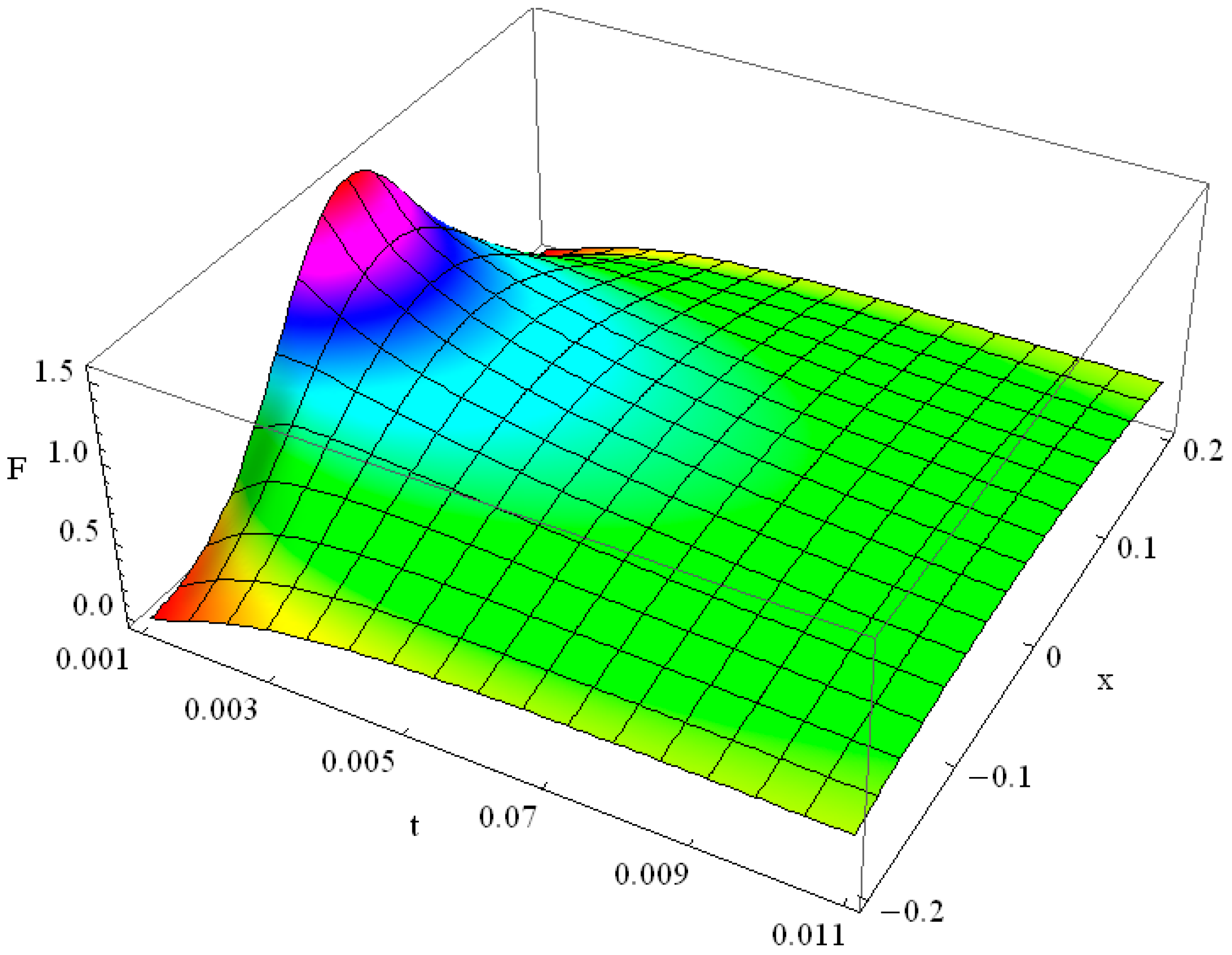
Consider the Equation (13) for , . This case represents the Fourier heat propagation, including heat exchange with the environment. Consider the flash initial condition for it. The solution is shown in Figure 1 and it evidences significant spread of the initial function already for the times .
The plot in Figure 1 is compiled for α = 1, γ = 1, which represents the Fourier heat solution with some heat exchange with the environment. At the moment t = 0.001 we see the Gaussian as the result of the evolution of the δ-function; at the moment t = 0.01 this Gaussian has faded and the contribution of the heat exchange term γ is noticeable. The relaxed solution slowly grows due to non-zero heat exchange with .
4. Operational Solution of the Hyperbolic Heat Conduction Equation
The Fourier heat law [75] has some shortcomings, noted by L. Onsager in 1931, who said [80] that it “contradicts the principle of microscopic reversibility, but this contradiction is removed if we recognize that it is only an approximate description of the process of conduction, neglecting the time needed for acceleration of the heat flow”. The Fourier law does not properly describe heat conduction at low temperature <25 K in dielectric crystals and in systems with reduced dimensions. Moreover, it has some unphysical properties, such as lack of inertia. In other words, if an instant temperature perturbation is applied at a point in the solid, it will be felt everywhere instantaneously. This contradicts the phenomenon of the second sound, when the temperature perturbation propagates like a wave with damping. To overcome these problems Cattaneo [76] proposed a time-dependent relaxational model, which yielded the following equation: , where DT is the heat conductivity and the relaxation time τ in heat conduction is extremely small (τ ≈ 10−13 s) at room temperature. This equation models the phenomenon of the second sound, first observed in liquid helium [81]. With the development of the second sound theoretical background [77], it was then later detected also in solid crystals [82,83,84,85]. In the relevant tests heat flash technology [79] was used for the sensitive measurement of the thermal diffusivity.
The application of the operational method for solution of the second order PDE was given in [72]. The following PDE with initial conditions:
where and are differential operators, acting over the coordinate, dependently on the specific form of the operators and , describes a variety of physical processes in thermodynamics, electrodynamics etc. The particular fading with time solution of Equation (18) formally reads as follows [72]:
The other solution of Equation (18) has a positive sign in the exponential: , and does not satisfy the requirement , which otherwise can be formulated as , i.e., the solution converges at infinite time. Both of these assumptions are reasonable for physical applications. We perform the Laplace transforms [41] in (19):
and, provided the integral converges, we obtain for Equation (18) the following vanishing at infinite time solution:
whose particular form depends on the differential operators , and on the initial condition . In what follows, we consider some examples.
Let us first of all consider and , keeping the linear term κ in the r.h.s. of Equation (18). Then we end with the telegraph equation, also known as a hyperbolic heat conduction equation (HHE):
Its fading at solution reads as follows:
The action of the heat diffusion operator can be accomplished with the help of the identity (4), resulting in
where . Consider an example of the initial function , which, is useful for the description of heat pulses of a variety of shapes, custom modelled by the sum . With the help of the operational identity (11) we obtain the exact form of the solution:
We omit the bulky result of the above integration for arbitrary , which can be computed with account for (9). In the particular case of given n and γ, for the example for , we obtain
For , , we have the following solution:
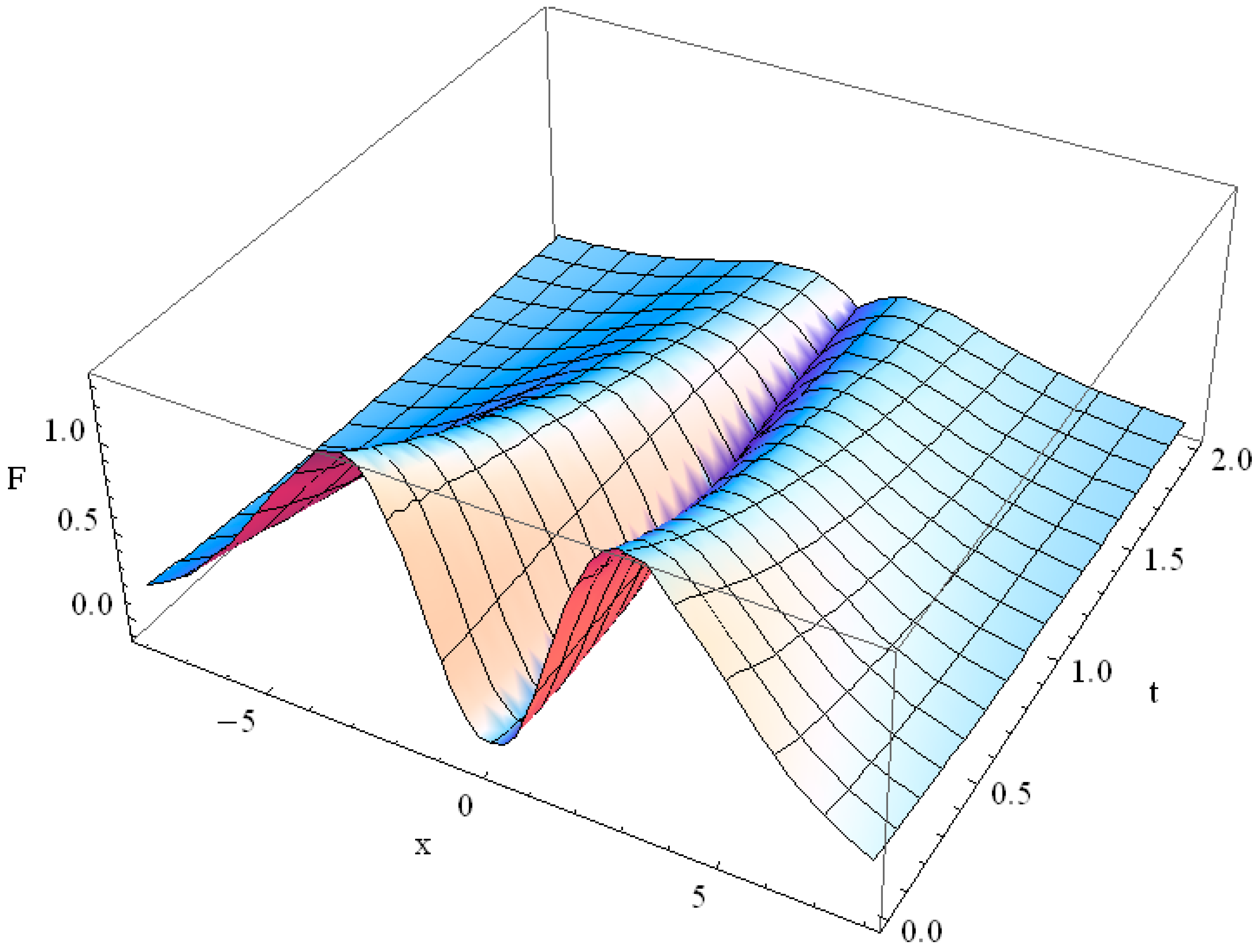
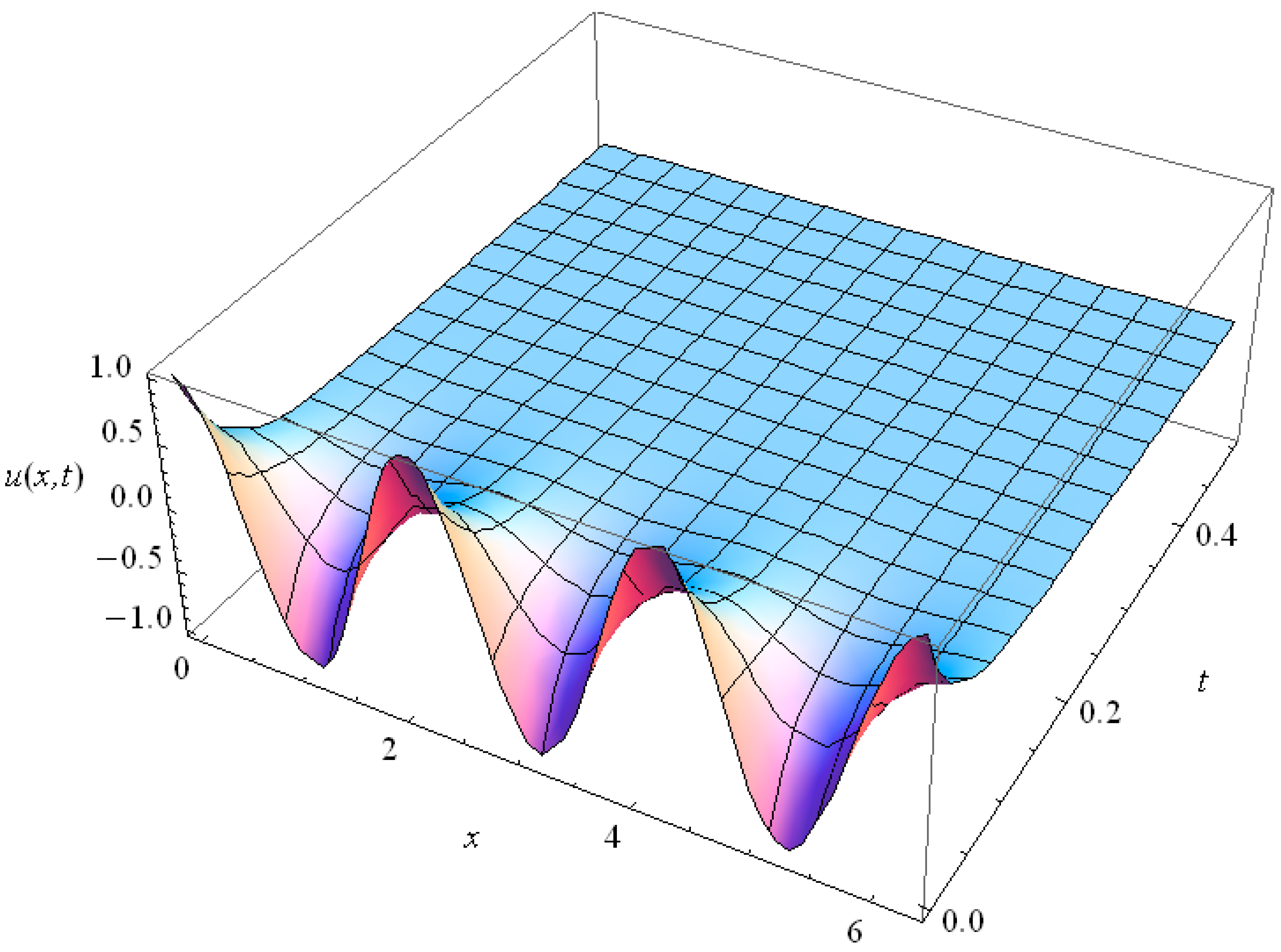
The solution for the initial function is too bulky to be presented in its analytical form; it describes the damped wave propagation as shown in Figure 2.
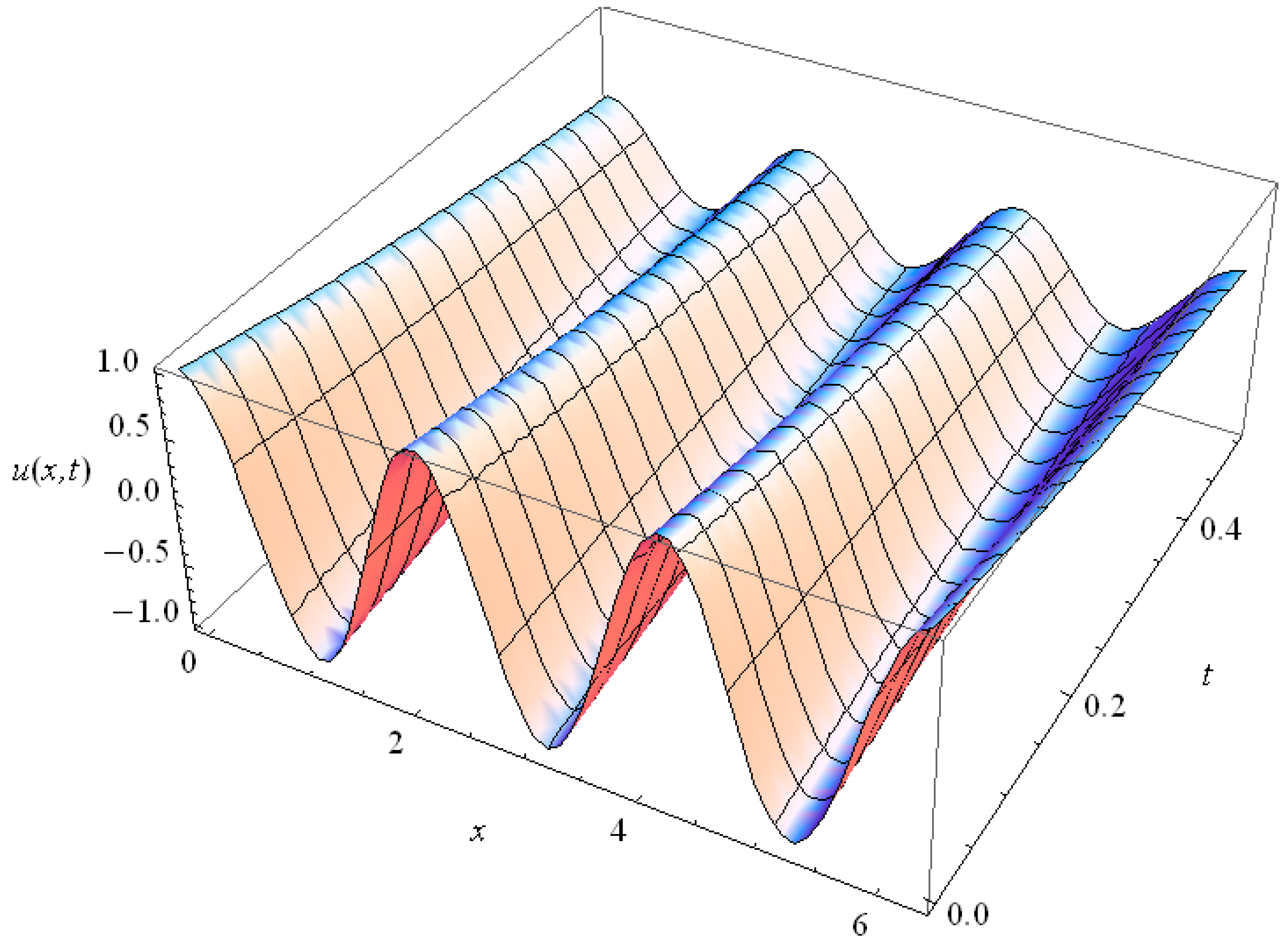
By choosing in (22), i.e., , , the influence of the second time derivative in the Cattaneo equation is reduced, but the heat conductivity remains unchanged, as compared with the case . The relaxation of the solution occurs much earlier for , than for , as follows from the comparison of the plot in Figure 2 with that in Figure 3; the reason is that the diffusive heat transfer in this case prevails over the wave heat transfer.
5. Propagation of a Heat Surge with the Hyperbolic Heat Conduction Equation
We now consider the example of initial δ-function for Equation (22). The action of the operator in our solution (23) can be accomplished with the help of Equation (16), where , as follows: . Now the integration in (23) can be completed for the times , where the solution exists:
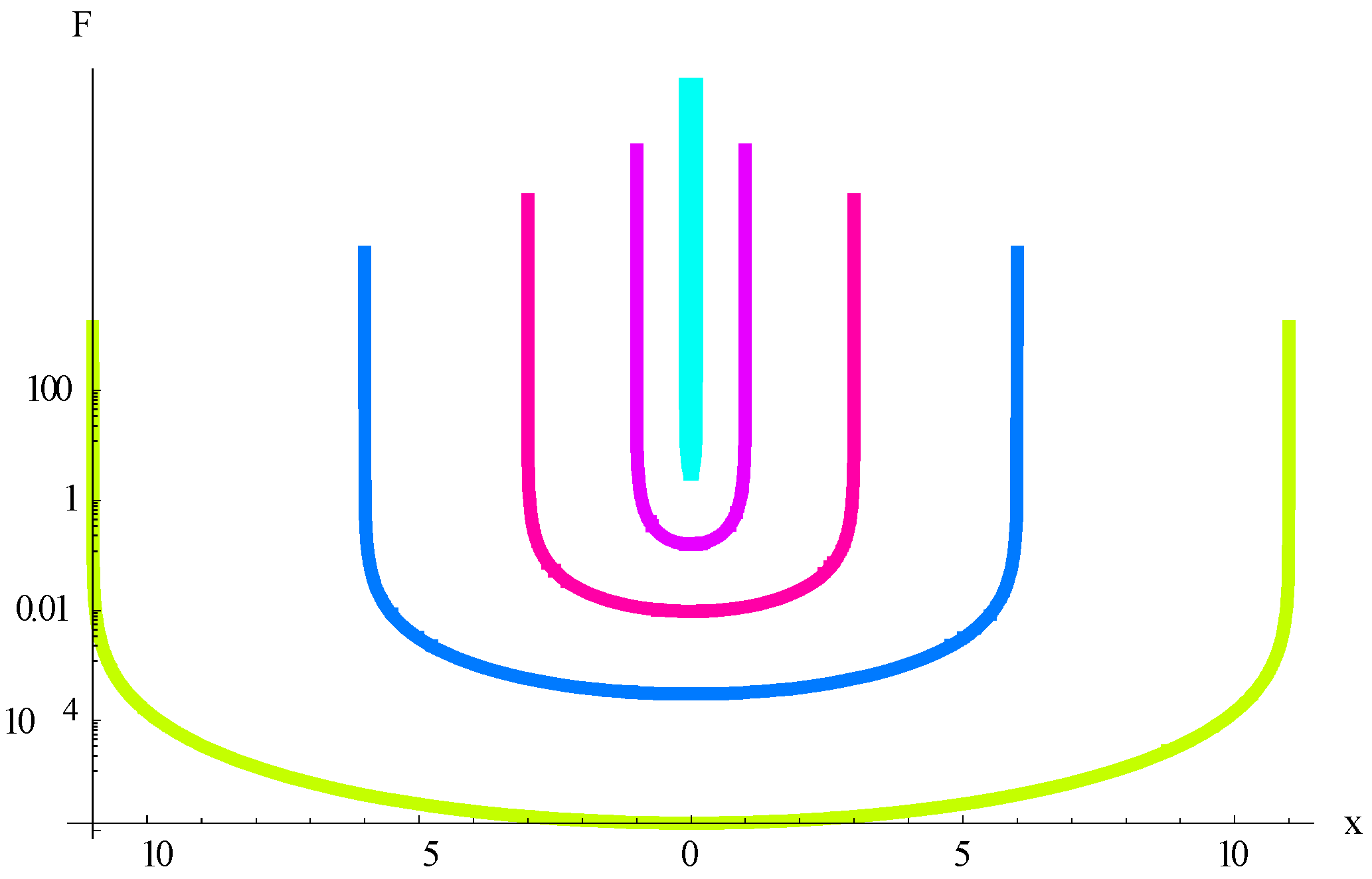
Physical meaning of the condition , i.e., is that the time, needed for the initial δ(x) function to reach the point x in space, is exactly and before that the heat surge is just not felt in the point x at all. The value is the velocity of the surge propagation, finite in the Cattaneo model, contrary to the infinite signal propagation speed in the Fourier law. The solution of Equation (22) for for the initial function is shown in Figure 4 for the moments of time t = 0.01 (light blue line), t = 0.1 (lilac line), t = 0.3 (pink line), t = 0.6 (blue line) and t = 1.1 (yellow–green line). Differently from the Fourier law, the initial flash reaches the point x at the moment and there is still no non-trivial solution in the point x before this moment of time. The initial δ-function is not shown in Figure 4 because of its infinite amplitude.
Higher values of α and ε reduce the contribution of the second order time-derivative in the Cattaneo Equation respectively to the role of other terms in (22). The damping of the solution in this case occurs sooner. We omit the proper plot for conciseness. Note that in the case of negative κ, i.e., when positive κ is in the l.h.s. of the hyperbolic Equation (22), the integral in (28) converges for , . Interestingly, despite the fact that the solution (28) was obtained for , it holds true for any . For we obtain positive values for , while for as well as for we obtain complex values for the resulting function . For we obtain . For the solution (28) diverges.
Heat propagation in three spatial dimensions in the Cattaneo model is governed by the direct three-dimensional generalization of (22) for κ = 0: , where is the heat conductivity. The ratio has the dimension of velocity and it stands for the speed of the heat wave propagation in the medium, τ is the material parameter, describing the time, needed for the initiation of a heat flow after a temperature gradient was imposed at the boundary of the domain. Thus, it determines the time lag for the appearance or disappearance of the heat flow after the temperature gradient is imposed or removed. This relaxation time is associated in the framework of the Cattaneo model with the linkage time of phonon-phonon collision and it measures the thermal inertia of the medium through the time, needed for the heat flow to fade in or out. The role of the constant term in the HHE becomes clearer in the context of the signal propagation in long telephone lines. We will consider it in what follows. At the moment we will keep for generality the constant term in the three-dimensional telegraph equation, thus writing it as follows:
where is the thermal diffusivity, k is the thermal conductivity, ρ is the mass density, cp is the specific heat capacity, is the relaxation time, often related to the speed of the second sound C in media: . The operational solution of (29) includes the action of the heat diffusion operators for each coordinate on the initial function:
The action of , where is easy to obtain: the result for each coordinate heat operator action is given by the inner integral in (24) and then the integration over can be performed if the integral converges.
For experimental measurement of the thermal conductivity the flash technique is commonly approved. For this reason we choose the initial function , modelling an intense instant point-like volume heating. The application of the heat operators gives yields the following solution for HHE (29) with :
The above integral converges for and we obtain the following simple analytical expression, involving modified Bessel functions K2:
Note, that the above solution also holds for . As well as in the one-dimensional case (28) for , that is for the times, inferior , when the heat wave reaches point x, we obtain positive values for the solution for negative κ, such that . For as well as for we obtain complex solution . In the limiting case of we obtain the finite limit for the solution: , but for the solution diverges.
Despite that the Cattaneo heat Equation (22) for is reversible on the time scale of the thermal relaxation time τ, and despite that it predicts a finite value for the heat wave velocity , its quantitative value disagrees with the experimental data at high frequencies and low temperatures. However, the HHE is widely used in radio engineering.
6. Propagation of a Harmonic Signal with the Telegraph Equation
In the context of signal propagation in cable lines without radiation loss the HHE (22) is perfectly usable for the description of the voltage and current 86. For this reason we choose the initial harmonic function . The action of the operator with account for (5) yields , . Integration in (24) in turn yields the following solution for the telegraph Equation (22) for :
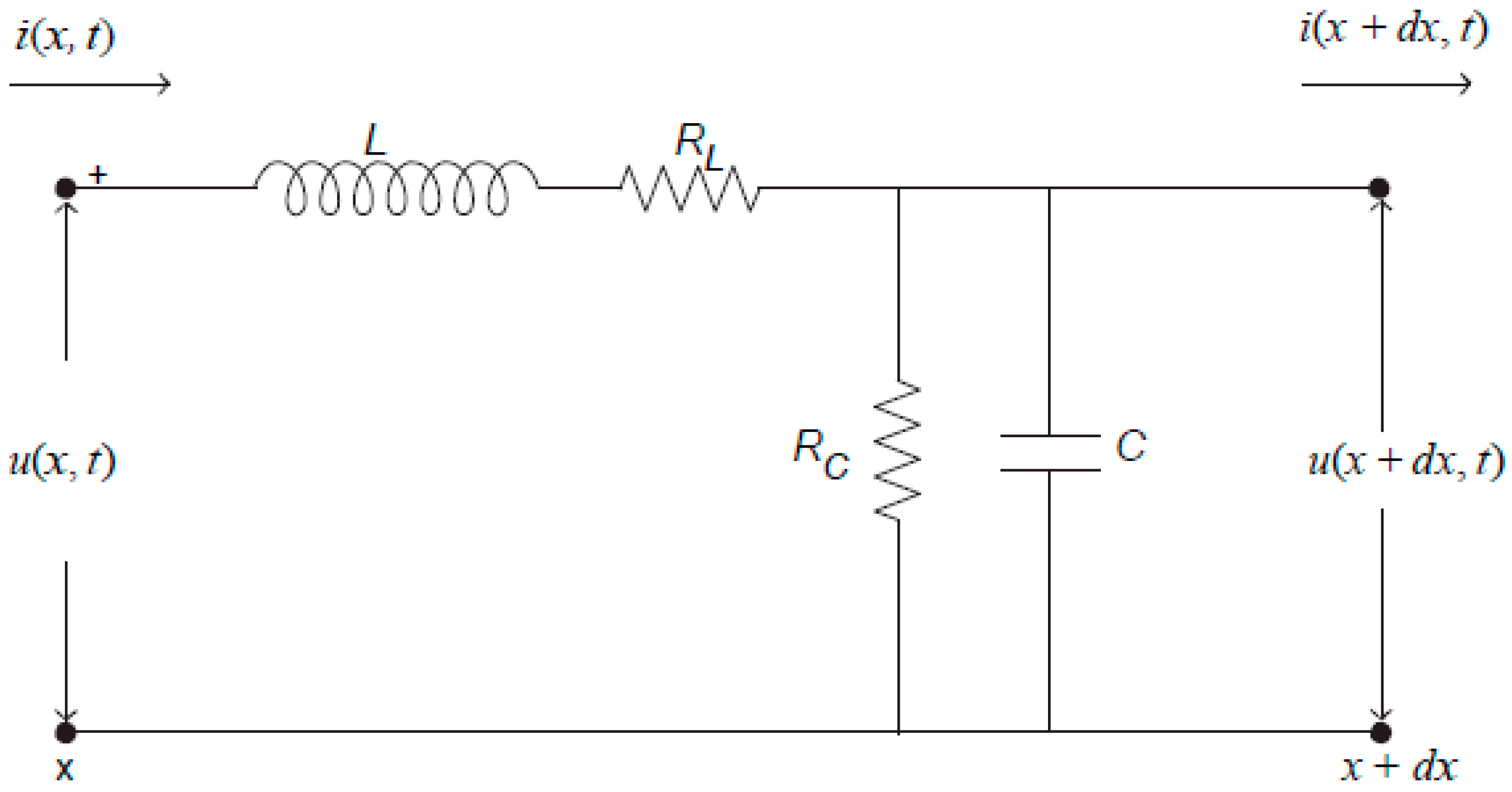
The harmonic solution (33) is not spreading in space, but only fading in time. Its physical meaning is clarified if we attribute the constants in HHE (22) the values according to the schematic diagram of the electric circuit in Figure 5, where the electric line with finite resistance, inductivity, capacitance, and leakage is shown.
In terms of the resistance RL, inductivity L, capacitance C and leakage resistance RC the voltage along the transmission line, shown in Figure 5, is described by the one-dimensional telegraph equation [86]:
In our notations , and . The solutions (28) and (32) for the initial δ-surge are valid and converge also for provided .
For the periodic solution (33) is realized; it fades without the space shift (see examples in Figure 6). In the case of the voltage behavior in the circuit has space shift and its time fading depends exclusively on (see examples in Figure 7):
The essential difference between the plots in Figure 6 and Figure 7 is in the time dependent spatial phase shift, which is seen in Figure 7 for and is absent in Figure 6 for .
Thus the first three harmonics for RC = 7, C = L = RL = 1 develop in time without the space shift with decent fading (see examples for n = 2, 3 in Figure 6); for them the solution (33) is realized. The harmonics with are governed by the solution (35), they have a time-dependent space shift (see examples for n = 4, 5 in Figure 7). With increase of n the relaxation time of the harmonics also increases, but from a certain harmonic, for which the space shift appears, the relaxation time stabilizes and remains equal for all higher harmonics. In the context of heat conduction it means that the heat conduction for higher harmonics is lower than the heat conduction for low harmonics. It may also occur that, dependent on the values of the parameters in the HHE all harmonics have time-dependent space shift, i.e., the solution (35) is realized for . This frequency dependent heat conductivity is typical for HHE and it is absent in the Fourier law.
Concluding the study of the hyperbolic heat Equation (22) we note that it can be easily modified by adding non-commuting with terms and mixed derivatives over time and coordinate. Such a modified hyperbolic equation can be solved with the help of the above developed operational technique.
7. Operational Solution of Guyer-Krumhansl Type Heat Equation and Heat Conduction in Thin Films
The Cattaneo hyperbolic equation gives a qualitatively correct description of the second sound through the heat wave propagation at finite velocity, but numerical results do not match the experiment. The predicted values for the speed of the heat wave in matter disagree with the data on ultrasonic wave propagation in dilute gases. Neither the heat pulse propagation at very low temperature is described correctly in non-metallic very pure crystals of Bi and Na F. In response to this disagreement, further generalizations of the Fourier law were developed. Among them the Guyer-Krumhansl (GK) equation [87] is distinguished for simplicity and coherence with observed data. In addition to the heat waves the GK model takes into consideration the so-called ballistic transport, which can be observed when the mean free path of a particle significantly exceeds the dimension of the medium in which it travels. The mean free path increases at low temperatures For example, for electrons in a medium with negligible electrical resistance, their motion is altered by collisions with the walls. Ballistic conduction applies also to phonons. It is typically observed in low dimensional structures, such as very thin films, silicon nanowires, carbon nanotubes, graphene etc. (see, for example, [88,89,90,91,92]). When the bulk phonon mean free path l is comparable to the structure size L, neither the Casimir phonon theory [93] nor Fourier diffusion [75] describe the heat transfer well, which is affected by boundary as well as internal scattering. The common rule that determines which type of transport dominates is the following: when l << L, the heat diffusion prevails, but for l >> L, or when the temperature gradient becomes large, the ballistic transport cannot be ignored. Recently the conditions for the transition region between the ballistic heat transport and the diffusion were described in [92]. Whether the heat transfer is ballistic or diffusive is also important for experimentalists, because the account for the ballistic phonon transport requires the knowledge of the boundary quality, while the wave and diffusive transport constants are intrinsic material properties [94,95,96]. The three dimensional Guyer-Krumhansl (GK) heat law was derived from the solution of the linearized Boltzmann equation for a phonon field in dielectric crystals at low temperature. It is good for the description of phonon gases in low temperature samples and even for some heat propagation processes on the microscopic [97] and macroscopic [98,99,100,101,102] level at room temperature [103,104,105]. The relaxation of the laser flash was shown to follow the GK law [106], which was reconsidered in the framework of weakly non-local thermodynamics in [107]. Due to the wide interest in the GK equation and its relatively good agreement with an array of experiments over a broad temperature range, conducted in various materials, we will consider the GK equation solution for propagation of spatial heat waves and flash pulses. To this end we will use the operational technique.
Let us choose the operators and in (18), which results in the following GK type equation with mixed derivative:
The one-dimensional GK equation is essentially Equation (36) with κ = 0; we will keep for the sake of generality. Its role is not indifferent and it will be discussed in what follows. Introducing the operators and , we can rewrite (36) with positive coefficients in the following form:
Note that equations represent Fourier law. If and , we have , and, provided the Fourier Equation is fulfilled, we have the particular case of GK equation, which is Equation (37) with , also satisfied by this solution . The form of the heat conduction equation Equation (36) with arises in the study of heat propagation in a one-dimensional thin film with account for the phonon transport [108]. From (21), where , , we write the solution of Equation (36) as follows:
By means of the integral presentation (see (5)) we obtain after grouping the 2nd order derivative terms in the exponential the particular bounded solution for the modified hyperbolic heat conduction Equation (36) with initial function as follows:
where , , . Note, that the obtained integral solution is valid also if the constant term in the r.h.s. of the Equation (36) is negative: and , which insures the integral convergence. Equations with negative sign of κ have sense and they arise for ballistic heat propagation in thin films [108].
The application of the above solution is direct: it was demonstrated that heat propagation in thin films obeys the extended form of GK Equation (36). In particular, the following equation for thin films was proposed [108]:
where is the ballistic component of the dimensionless energy (or quasi-temperature) and Kn is the Knudsen number, describing the molecular and the boundary effects. Equation (40) is a GK type Equation (36) with the following coefficients: , , , .
In what follows, we will consider some examples of heat pulse propagation.
8. Propagation of a Heat Surge with the Guyer-Krumhansl Heat Equation
Consider the example of the initial flash , corresponding to an intense and instant laser point heating at at the moment of time . From Equation (16) for we obtain . Then from (39) the analytical solution of GK type Equation (36) with follows:
where we denote the special function
Function reduces for some particular values of a and b to the hypergeometric function , this last being the particular case of . Moreover, and . The numerical calculation of the double integral (41), taken with care around the point a = 0, corresponding to the time , yields real values. The example of the solution (41) of the GK type Equation (36) with for the initial flash is shown in Figure 8.
From the comparison of Figure 8 with Figure 1 we conclude that the solution of the Fourier heat Equation (1) (see Figure 1) is more pronounced at short times, it has a higher peak, while the solution of GK Equation (36) spreads faster (see Figure 8) when the additional terms ε = δ = 1 are comparable with the others order.
In the context of heat conduction in thin films we solved the respective GK equation for and for . The results for the ballistic dimensionless energy change after a laser pulse heating of a thin film, modelled by the GK type Equation (40), are shown in Figure 9 for Knudsen number Kn = 1 and in Figure 10 for Knudsen number Kn = 0.2. Their comparison confirms much faster heat propagation in a thin film with Kn = 1, where the ballistic transport mechanism contributes noticeably, as compared with the film with small value of Kn = 0.2.
9. Solution of the Guyer-Krumhansl Equation for the Exponential–Polynomial Initial Function
Interesting features of the heat conduction, governed by the Guyer-Krumhansl equation, arise from consideration of the evolution of the power–exponential initial function . Consideration of such a function is useful not only because it allows better approximation of experimental data than the usual polynomial and , γx < 0, but also as itself it represents a pulse, and practically any solitary space wave or surge is easy to approximate by its sum . The operational method allows the exact analytical solutions for these functions to be obtained. Indeed, we make use of the operational identity (11) to obtain for , , . The solution for arbitrary values of can be obtained upon the following integration:
where , , , . The integration can be done in elementary functions if we account for the series presentation . We omit the final result for conciseness. For example, in the simplest case of , i.e., we obtain the following solution of the GK equation:
Let us now consider the initial smooth function . By means of the above developed operational technique we obtained the following exact analytical solution of the GK equation in elementary functions:
Direct substitution of the solution satisfies the GK equation. Earlier it was demonstrated that such solutions can show bizarre behavior with local maximums and local minimums even with negative values, occurring in the middle of the domain, so that theoretically for a certain set of parameters of the GK equation the maximum principle can be violated [58]. However, for applications, such as those in the thin films, modelled by the GK type Equation (40), there is no problem with the second law of thermodynamics violation. Indeed, the propagation of the smooth spatial heat distribution in the range of the values of the Knudsen number between changes no more than three percent.
The difference between these plots is not distinguishable visually and we present here just one example for in Figure 11. It corresponds to the values , . The behavior of the solution surprisingly resembles that for α ≈ ε ≈ δ ≈ 1, which we omit for brevity, as well as that for , for which , .
To contrast it, we demonstrate the behavior of the solution of GK equation (see (36), κ = 0) for relatively small contribution of the Cattaneo’s term: α = ε = δ = 10, which does not depend on the sign and on the exact value of the constant term κ (we omit proper figures with κ ≠ 0) for conciseness) and it has bizarre non-Fourier behavior, shown in Figure 12.
The initial pulse rapidly decreases and assumes negative values, then it gradually approaches zero. It maintains negative values in the whole space domain, but for the vicinity of . Around the solution becomes positive: and then it relaxes to zero: .
In this case, based on the obtained exact vanishing analytical solution of the GK equation with the initial function and , we conclude the minimum of the solution over the time-space domain is in the middle of the domain (see Figure 12). The local maximum of the solution may also occur in the middle of the domain (see [58,59]).
10. Harmonic Solution of Guyer-Krumhansl Equation and Temperature Distribution in Thin Films
The other good example of a given initial temperature distribution, is given by a harmonic function , which is necessary to consider approximations or expansion of the initial function into the Fourier series to fit experimental data distributions. The action of the heat conduction operator yields the following bounded at infinite times solution:
Upon integration we end up with the explicit solution of the GK Equations (36) and (37) for the periodic initial function , expressed in elementary functions as follows:
Interestingly, the solution (47) of GK type Equation (36) for the initial harmonic function repeats the solution of telegraph Equation (33) upon the substitution , where , in (33). In other words, the solution (47) of Equation GK type (36) for is also the solution of the HHE (22) with the harmonic dependent coefficient for the first order time derivative:
Thus, for the initial harmonic function and same values of the coefficients in Equations (36) and (48), these share identical particular solution (47). For the initial function , the solution of Equations (36) and (48) will be given by the series , where is the solution of (47). In this sense the GK type equation with the harmonic initial function can be viewed as the telegraph equation with the harmonic dependent coefficient for : and the GK equation for is in fact the Cattaneo equation for with instead of term. This radically changes the solution behavior. Indeed, the relaxation time for all higher harmonics in the telegraph Equation (33) is the same; only low harmonics may fade out faster. On the contrary, the solution (47) of the GK type Equation (36) for the harmonic function and the solution of the equivalent telegraph equation with (48) for high harmonics show that these harmonics fade out faster than the fundamental one (n = 1) and the higher the harmonic number n, the lower is its relaxation time. The examples for n = 3, 5 are shown in Figure 13.
Compare Figure 13 with the solution of the telegraph Equation (22) (see Figure 6 and Figure 7). High harmonics of the telegraph equation, shown in Figure 7, fade out slower than the low harmonics, shown in Figure 6. For the GK type equation or the HHE with on the contrary, high harmonics fade out faster than the fundamental and the low ones, as evidenced in Figure 13. The effective thermal conductivity in the common telegraph Equation (22) is constant for higher harmonics and in certain cases even for all n. On the contrary, in the GK type Equation (36), which is HHE with for (see (48)), the thermal conductivity for the harmonic function rises with increase of the harmonic number n.
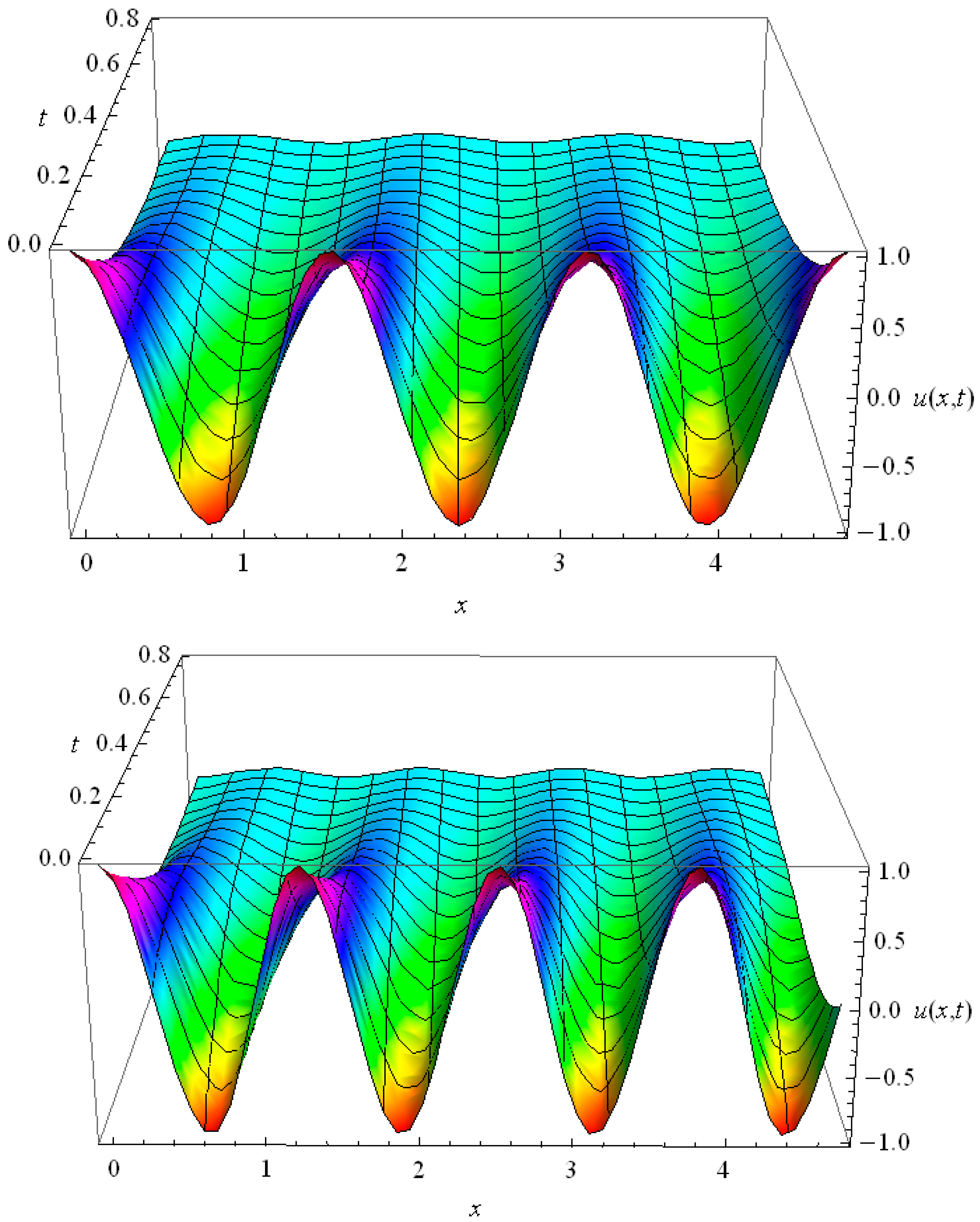
In the context of the heat conduction in thin films, for Kn = 1 we plotted the bounded solutions of Equation (40), for , n = 1, 3, in Figure 14 and Figure 15 respectively. High harmonics fade out rapidly as follows from their comparison with teach other. For Kn = 0.2 we present the solutions in Figure 16 and Figure 17 for n = 1, 3 respectively. The comparison with Figure 14, Figure 15 shows that the solutions for Kn = 0.2 relax much slower than those for Kn = 1.
This means that high values of the Knudsen number provide the ballistic transport contribution to the heat conduction, and the latter increases in the GK model, in particular, for high harmonics. The proper relaxation times for the first harmonic read as follows: n=1τKn=1 ≈ 0.5 and n=1τKn=0.2 ≈ 2.5; for the third harmonic the relaxation times are n=3τKn=1 ≈ 0.2 and n=3τKn=0.2 ≈ 3. The ratios of proper relaxation times are and . The heat conduction is evidently better for Kn = 1 than for Kn = 0.2.
11. Conclusions
We obtained exact analytical solutions for heat conduction in the Fourier, Cattaneo, and Guyer-Krumhansl heat transport models. Extended forms of these equations with additional constant terms were solved by the operational method. The obtained solutions directly satisfy the considered equations. The initial functions, modelling various types of pulses and signals were considered. The power–exponential pulse and the flash heat pulse were considered, modelling the laser heat pulse experimental technique, common for thermal conductivity measurements.
The analytical solutions were compared with each other. The finite speed of the heat propagation in the Cattaneo model was demonstrated. By reducing the effect of the second time derivative in the equation for , maintaining the heat conductivity unchanged, we obtain faster fading of the solution. In this case diffusive heat conduction prevails over the wave-like propagation process. On the contrary, for the wave-like propagation of the initial function dominates. For , both heat transport mechanisms contribute; the wave propagates at a constant speed, accompanied by fading.
The exact analytical solution of HHE in three space dimensions for initial flash was obtained in terms of modified Bessel functions. The HHE was solved with the harmonic initial function . The obtained solution fades in time exponentially and does not spread. The space phase shift of the solution depends on the sign of the linear term in HHE.
The GK type heat equation with linear term was solved operationally; the solution was written in terms of integrals and special functions. The propagation of the initial heat flash was studied and demonstrated for the model of heat conduction in thin films. Small values of Knudsen number result in slower relaxation of the initial heat surge; for the ballistic heat transport contributes and the heat surge fades out much faster. An exact solution for the evolution of the exponential-monomial function in the GK equation was obtained. This allows not only the propagation of a surge with power rise, followed by the common exponential fade, to be studied but also the result for the initial function to be obtained, which can be expanded in the series or approximated by them. The example of the initial smooth heat pulse relaxation in a thin film was considered.
We found that variation of the Knudsen number values in a reasonable range practically does not influence the relaxation time of the initial smooth pulse: the values of the solution of GK type equation vary less than 3% for . Thus in thin films the conditions on the surface, expressed by the Knudsen number, are particularly important for laser heat flash, but not that important for relaxation of a wide heat spot without a sharp boundary.
For the propagation of the initial laser heat flash the relaxation time is ten times smaller for Kn = 1 than for Kn = 0.2. The relaxation time τ for the harmonic initial function for the first harmonic (n = 1) is five times shorter for Kn = 1 than for Kn = 0.2: n=1τKn=1 ≈ 0.5 and n=1τKn=0.2 ≈ 2.5; for the third harmonic the relaxation time τ is 15 times shorter for Kn = 1 than τ for Kn = 0.2: the proper relaxation times are n=3τKn=1 ≈ 0.2 and n=3τKn=0.2 ≈ 3. The ratios of proper relaxation times are and .
We obtained exact analytical solutions in terms of the orthogonal polynomials and special functions for three different models of heat conduction: Fourier, Cattaneo, and Guyer-Krumhansl. These solutions allow analytical modelling of the space–time propagation for heat flashes and pulses, which is the established experimental technique. We can also model the relaxation of any initial function, expandable in the Fourier series and in the series of the exponential-polynomial function. This series approximation is applicable practically to any pulse.
In conclusion we stress that the operational technique, used for the solution of hyperbolic heat equations, yields exact analytical solutions. They have clear physical meaning and allow easy understanding of the role of different terms in the equations. The validity of the obtained analytical solutions was checked by their substitution in the equations, the latter were satisfied. Our study not only has theoretical interest, but it also provides practical results of experimental technique and measurements. The obtained exact analytical solutions can be used as a benchmark for numerical solutions of more sophisticated forms of the studied equations.
Conflicts of Interest
The author declares no conflict of interest.
References
- Von Rosenberg, D.U. Methods for the Numerical Solution of Partial Differential Equations; Society of Petroleum Engineers: Richardson, TX, USA, 1969; Volume 6. [Google Scholar]
- Smith, G.D. Numerical Solution of Partial Differential Equations: Finite Difference Methods; Oxford University Press: Oxford, UK, 1985. [Google Scholar]
- Ghia, U.; Ghia, K.N.; Shin, C.T. High-Re solutions for incompressible flow using the Navier-Stokes equations and a multigrid method. J. Comput. Phys. 1982, 48, 387–411. [Google Scholar] [CrossRef]
- Ames, W.F. Numerical Methods for Partial Differential Equations; Academic Press: Cambridge, MA, USA, 2014. [Google Scholar]
- Johnson, C. Numerical Solution of Partial Differential Equations by the Finite Element Method; Courier Corporation: Chelmsford, MA, USA, 2012. [Google Scholar]
- Carnahan, B.; Luther, H.A.; Wilkes, J.O. Applied Numerical Methods; John Wiley & Sons: Hoboken, NJ, USA, 1969. [Google Scholar]
- Spassky, D.; Omelkov, S.; Mägi, H.; Mikhailin, H.; Vasil’ev, A.; Krutyak, N.; Tupitsyna, I.; Dubovik, A.; Yakubovskaya, A.; Belsky, A. Energy transfer in solid solutions ZnxMg1−xWO4. Opt. Mater. 2014, 36, 1660–1664. [Google Scholar] [CrossRef]
- Kirkin, R.; Mikhailin, V.V.; Vasil’ev, A.N. Recombination of correlated electron-hole Pairs with account of hot capture with emission of optical phonons. IEEE Trans. Nuclear Sci. 2015, 59, 2057–2064. [Google Scholar] [CrossRef]
- Gridin, S.; Belsky, A.; Dujardin, C.; Gektin, A.; Shiran, N.; Vasil’ev, A. Kinetic model of energy relaxation in Csl:A (A = Tl and In) scintillators. J. Phys. Chem. C 2015, 119, 20578–20590. [Google Scholar] [CrossRef]
- Krutyak, N.R.; Mikhailin, V.V.; Vasil’ev, A.N.; Spassky, D.A.; Tupitsyna, I.A.; Dubovik, А.M.; Galashov, E.N.; Shlegel, V.N.; Belsky, A.N. The features of energy transfer to the emission centers in ZnWO4 and ZnWO4:Mo. J. Lumin. 2013, 144, 105–111. [Google Scholar] [CrossRef]
- Savon, A.E.; Spassky, D.A.; Vasil’ev, A.N.; Mikhailin, V.V. Numerical simulation of energy relaxation processes in a ZnMoO4 single crystal. Opt. Spectrosc. 2012, 112, 72–78. [Google Scholar] [CrossRef]
- Denisov, V.I.; Shvilkin, B.N.; Sokolov, V.A.; Vasili’ev, M.I. Pulsar radiation in post-Maxwellian vacuum nonlinear electrodynamics. Phys. Rev. D 2016, 94, 45021. [Google Scholar] [CrossRef]
- Denisov, V.I.; Sokolov, V.A. Analysis of regularizing properties of nonlinear electrodynamics in the Einstein-Born-Infeld theory. J. Exp. Theor. Phys. 2011, 113, 926–933. [Google Scholar] [CrossRef]
- Denisov, V.I.; Sokolov, V.A.; Vasiliev, M.I. Nonlinear vacuum electrodynamics birefringence effect in a pulsar’s strong magnetic field. Phys. Rev. D 2014, 90, 023011. [Google Scholar] [CrossRef]
- Denisov, V.I.; Kozar, A.V.; Sharikhin, V.F. Investigation of the trajectories of a magnetized particle in the equatorial plane of a magnetic dipole. Mosc. Univ. Phys. Bull. 2010, 65, 164–169. [Google Scholar] [CrossRef]
- Vladimirova, Y.V.; Zadkov, V.N. Frequency modulation spectroscopy of coherent dark resonances of multi-level atoms in a magnetic field. Mosc. Univ. Phys. Bull. 2010, 65, 493. [Google Scholar] [CrossRef]
- Yanyshev, D.N.; Balykin, V.I.; Vladimirova, Y.V.; Zadkov, V.N. Dynamics of atoms in a femtosecond optical dipole trap. Phys. Rev. A 2013, 87, 033411. [Google Scholar] [CrossRef]
- Bulin, A.-L.; Vasil’ev, A.; Belsky, A.; Amans, D.; Ledoux, G.; Dujardin, C. Modelling energy deposition in nanoscintillators to predict the efficiency of the X-ray-induced photodynamic effect. Nanoscale 2015, 7, 5744–5751. [Google Scholar] [CrossRef] [PubMed]
- Pastukhov, V.M.; Vladimirova, Y.V.; Zadkov, V.N. Photon-number statistics from resonance fluorescence of a two-level atom near a plasmonic nanoparticle. Phys. Rev. A 2014, 90, 063831. [Google Scholar] [CrossRef]
- Gong, L.; Zhao, J.; Huang, S. Numerical study on layout of micro-channel heat sink for thermal management of electronic devices. Appl. Therm. Eng. 2015, 88, 480–490. [Google Scholar] [CrossRef]
- Xia, G.; Ma, D.; Zhai, Y.; Li, Y.; Liu, R.; Du, M. Experimental and numerical study of fluid flow and heat transfer characteristics in microchannel heat sink with complex structure. Energy Convers. Manag. 2015, 105, 848–857. [Google Scholar] [CrossRef]
- Wang, R.; Du, J.; Zhu, Z. Effects of wall slip and nanoparticles’ thermophoresis on the convective heat transfer enhancement of nanofluid in a microchannel. J. Thermal Sci. Technol. 2016, 11, JTST00017. [Google Scholar] [CrossRef]
- Roy, R.; Ghosal, S. Homotopy perturbation method for the analysis of heat transfer in an annular fin with temperature-dependent thermal conductivity. J. Heat Transfer 2016, 139, 022001. [Google Scholar] [CrossRef]
- Demiray, S.T.; Bulut, H.; Belgacem, F.B. Sumudu transform method for analytical solutions of fractional type ordinary differential equations. Math. Probl. Eng. 2015, 2015, 131690. [Google Scholar]
- Mathai, A.M. M-convolutions of products and ratios, statistical distributions and fractional calculus. Analysis 2016, 36, 15–26. [Google Scholar] [CrossRef]
- Saxena, R.K.; Mathai, A.M.; Haubold, H.J. Computational solutions of unified fractional reaction-diffusion equations with composite fractional time derivative. Commun. Nonlinear Sci. Numer. Simul. 2015, 27, 1–11. [Google Scholar] [CrossRef]
- Mathai, A.M. Fractional integral operators in the complex matrix variate case. Linear Algebra Appl. 2013, 439, 2901–2913. [Google Scholar] [CrossRef]
- Haubold, H.J.; Mathai, A.M.; Saxena, R.K. Further solutions of fractional reaction-diffusion equations in terms of the H-function. J. Comput. Appl. Math. 2011, 235, 1311–1316. [Google Scholar] [CrossRef]
- Mathai, A.M. Fractional differential operators in the complex matrix-variate case. Linear Algebra Appl. 2015, 478, 200–217. [Google Scholar] [CrossRef]
- Akinlar, M.A.; Kurulay, M. A novel method for analytical solutions of fractional partial differential equations. Math. Probl. Eng. 2013, 2013, 195708. [Google Scholar] [CrossRef]
- Mathai, A.M.; Saxena, R.K.; Haubold, H.J. A certain class of Laplace transforms with applications to reaction and reaction-diffusion equations. Astrophys. Space Sci. 2006, 305, 283–288. [Google Scholar] [CrossRef]
- Zhukovsky, K.V. Operational solution for non-integer ordinary and evolution type partial differential equations. Axioms 2016, in press. [Google Scholar]
- Saxena, R.K.; Mathai, A.M.; Haubold, H.J. Solutions of certain fractional kinetic equations and a fractional diffusion equation. J. Math. Phys. 2010, 51, 103506. [Google Scholar] [CrossRef]
- Filobello-Nino, U.; Vazquez-Leal, H.; Benhammouda, B.; Perez-Sesma, A.; Jimenez-Fernandez, V.M.; Cervantes-Perez, J.; Sarmiento-Reyes, A.; Huerta-Chua, J.; Morales-Mendoza, L.J.; Gonzalez-Lee, M.; et al. Analytical solutions for systems of singular partial differential-algebraic equations. Discret. Dyn. Nat. Soc. 2015, 2015, 752523. [Google Scholar] [CrossRef]
- Benhammouda, B.; Vazquez-Leal, H. Analytical solutions for systems of partial differential-algebraic equations. SpringerPlus 2014, 3, 137. [Google Scholar] [CrossRef] [PubMed]
- Hesam, S.; Nazemi, A.R.; Haghbin, A. Analytical solution for the Fokker-Planck equation by differential transform method. Sci. Iran. 2012, 19, 1140–1145. [Google Scholar] [CrossRef]
- Vitanov, N.K.; Dimitrova, Z.I.; Vitanov, K.N. Modified method of simplest equation for obtaining exact analytical solutions of nonlinear partial differential equations: Further development of the methodology with applications. Appl. Math. Comp. 2015, 269, 363–378. [Google Scholar] [CrossRef]
- Bateman, H.; Erdélyi, A.; Magnus, W.; Oberhettinger, F.; Tricomi, F.G. Higher Transcendental Functions; McGraw-Hill Book Company: New York, NY, USA; 1953; Volume II. [Google Scholar]
- Mathai, M.; Saxena, R.K.; Haubold, H.J. The H-Function: Theory and Applications; Springer Science & Business Media: Berlin, Germany, 2009. [Google Scholar]
- Mathai, A.M.; Haubold, H.J. Special Functions for Applied Scientists; Springer Science & Business Media: Berlin, Germany, 2008. [Google Scholar]
- Wolf, K.B. Integral Transforms in Science and Engineering; Plenum Press: New York, NY, USA, 1979. [Google Scholar]
- Dattoli, G.; Srivastava, H.M.; Zhukovsky, K. A new family of integral transforms and their applications, Integral Transform. Integral Transform Spec. Funct. 2006, 17, 31–37. [Google Scholar] [CrossRef]
- Appèl, P.; de Fériet, J.K. Fonctions Hypergéométriques et Hypersphériques; Polynômes d’Hermite; Gauthier-Villars: Paris, France, 1926. [Google Scholar]
- Dattoli, G.; Srivastava, H.M.; Zhukovsky, K. Оrthogonality properties of the Hermite and related polynomials. J. Comput. Appl. Math. 2005, 182, 165–172. [Google Scholar] [CrossRef]
- Dattoli, G. Generalized polynomials, operational identities and their applications. J. Comput. Appl. Math. 2000, 118, 111–123. [Google Scholar] [CrossRef]
- Dattoli, G.; Srivastava, H.M.; Zhukovsky, K.V. Operational methods and differential equations with applications to Initial-Value problems. Appl. Math. Comput. 2007, 184, 979–1001. [Google Scholar] [CrossRef]
- Dattoli, G.; Mikhailin, V.V.; Zhukovsky, K.V. Influence of a constant magnetic field on the radiation of a planar undulator. Mosc. Univ. Phys. Bull. 2009, 64, 507–512. [Google Scholar] [CrossRef]
- Dattoli, G.; Mikhailin, V.V.; Zhukovsky, K. Undulator radiation in a periodic magnetic field with a constant component. J. Appl. Phys. 2008, 104, 124507. [Google Scholar] [CrossRef]
- Zhukovsky, K. Analytical account for a planar undulator performance in a constant magnetic field. J. Electromagn. Waves Appl. 2014, 28, 1869–1887. [Google Scholar] [CrossRef]
- Zhukovsky, K.V. Harmonic radiation in a double-frequency undulator with account for broadening. Mosc. Univ. Phys. Bull. 2015, 70, 232–239. [Google Scholar] [CrossRef]
- Zhukovsky, K. High harmonic generation in undulators for FEL. Nucl. Instr. Meth. B 2015, 369, 9–14. [Google Scholar] [CrossRef]
- Zhukovsky, K.V. Harmonic generation by ultrarelativistic electrons in a planar undulator and the emission-line broadening. J. Electromagn. Waves Appl. 2015, 29, 132–142. [Google Scholar] [CrossRef]
- Zhukovsky, K. High harmonic generation in the undulators for free electron lasers. Opt. Commun. 2015, 353, 35–41. [Google Scholar] [CrossRef]
- Zhukovsky, K. Emission and tuning of harmonics in a planar two-frequency undulator with account for broadening. Laser Part. Beams 2016, 34, 447–456. [Google Scholar] [CrossRef]
- Haimo, D.T.; Markett, C. A representation theory for solutions of a higher-order heat equation, I. J. Math. Anal. Appl. 1992, 168, 89–107. [Google Scholar] [CrossRef]
- Haimo, D.T.; Markett, C. A representation theory for solutions of a higher-order heat equation, II. J. Math. Anal. Appl. 1992, 168, 289–305. [Google Scholar] [CrossRef]
- Zhukovsky, K.V. Exact solution of Guyer-Krumhansl type heat equation by operational method. Int. J. Heat Mass Transfer 2016, 96, 132–144. [Google Scholar] [CrossRef]
- Zhukovsky, K.V. Violation of the maximum principle and negative solutions with pulse propagation in Guyer-Krumhansl model. Int. J. Heat Mass Transfer 2016, 98, 523–529. [Google Scholar] [CrossRef]
- Zhukovsky, K.V.; Srivastava, H.M. Analytical solutions for heat diffusion beyond Fourier law. Appl. Math. Comp. 2007, 293, 423–437. [Google Scholar] [CrossRef]
- Dattoli, G.; Zhukovsky, K.V. Quark flavour mixing and the exponential form of the Kobayashi-Maskawa matrix. Eur. Phys. J. C 2007, 50, 817–821. [Google Scholar] [CrossRef]
- Dattoli, G.; Zhukovsky, K. Quark mixing in the standard model and the space rotations. Eur. Phys. J. C 2007, 52, 591–595. [Google Scholar] [CrossRef]
- Dattoli, G.; Zhukovsky, K. Quark mixing and the exponential form of the Kobayashi-Maskawa matrix. Phys. Atom. Nucl. 2008, 71, 1807–1812. [Google Scholar] [CrossRef]
- Dattoli, G.; Zhukovsky, K.V. Neutrino Mixing and the exponential form of the Pontecorvo-Maki-Nakagawa-Sakata matrix. Eur. Phys. J. C 2008, 55, 547–552. [Google Scholar] [CrossRef]
- Zhukovsky, K.; Borisov, A. Exponential parameterization of neutrino mixing matrix—Comparative analysis with different data sets and CP violation. Eur. Phys. J. C. 2016, in press. [Google Scholar] [CrossRef]
- Zhukovsky, K.; Melazzini, F. Exponential parameterization of neutrino mixing matrix with account of CP-violation data. Eur. Phys. J. C 2016, 76, 462. [Google Scholar] [CrossRef]
- Haubold, H.J.; Mathai, A.M.; Saxena, R.K. Analysis of solar neutrino data from Super-Kamiokande I and II. Entropy 2014, 16, 1414–1425. [Google Scholar] [CrossRef]
- Mathai, A.M.; Haubold, H.J. On a generalized entropy measure leading to the pathway model with a preliminary application to solar neutrino data. Entropy 2013, 15, 4011–4025. [Google Scholar] [CrossRef]
- Mathai, A.M.; Saxena, R.K.; Haubold, H.J. Back to the solar neutrino problem. Space Res. Today 2012, 185, 112–123. [Google Scholar]
- Zhukovsky, K. Solution of some types of differential equations: Operational calculus and inverse differential operators. Sci. World J. 2014, 2014, 454865. [Google Scholar] [CrossRef] [PubMed]
- Zhukovsky, K.V. A method of inverse differential operators using ortogonal polynomials and special functions for solving some types of differential equations and physical problems. Mosc. Univ. Phys. Bull. 2015, 70, 93–100. [Google Scholar] [CrossRef]
- Zhukovsky, K.V.; Dattoli, G. Evolution of non-spreading Airy wavepackets in time dependent linear potentials. Appl. Math. Comp. 2011, 217, 7966–7974. [Google Scholar] [CrossRef]
- Zhukovsky, K. Operational solution for some types of second order differential equations and for relevant physical problems. J. Math. Anal. Appl. 2017, 446, 628–647. [Google Scholar] [CrossRef]
- Zhukovsky, K.V. Operational solution of differential equations with derivatives of non-integer order, Black-Scholes type and heat conduction. Mosc. Univ. Phys. Bull. 2016, 71, 237–244. [Google Scholar] [CrossRef]
- Gould, H.W.; Hopper, A.T. Operational formulas connected with two generalizations of Hermite polynomials. Duke Math. J. 1962, 29, 51–63. [Google Scholar] [CrossRef]
- Fourier, J.P.J. The Analytical Theory of Heat; Cambridge University Press: London, UK, 1878. [Google Scholar]
- Cattaneo, C. Sur une forme de l’equation de la chaleur eliminant le paradoxe d’une propagation instantanee. Comptes Rendus Hebdomadaires des Séances de l'Académie des Sciences 1958, 247, 431–433. [Google Scholar]
- Guyer, R.A.; Krumhansl, J.A. Solution of the linearized phonon Boltzmann equation. Phys. Rev. 1966, 148, 766–778. [Google Scholar] [CrossRef]
- Srivastava, H.M.; Manocha, H.L. A Treatise on Generating Functions; Ellis Horwood Limited: Chichester, UK, 1984. [Google Scholar]
- Parker, W.J.; Jenkins, R.J.; Butler, C.P.; Abbott, G.L. Flash method of determining thermal diffusivity, heat capacity, and thermal conductivity. J. Appl. Phys. 1961, 32, 1679. [Google Scholar] [CrossRef]
- Onsager, L. Reciprocal Relations in irreversible processes. Phys Rev. 1931, 37, 119. [Google Scholar] [CrossRef]
- Peshkov, V. Second sound in Helium II. J. Phys. (Mosc.) 1944, 8, 381. [Google Scholar]
- Ackerman, C.; Guyer, R.A. Temperature pulses in dielectric solids. Ann. Phys. 1968, 50, 128–185. [Google Scholar] [CrossRef]
- Ackerman, C.; Overton, W.C. Second sound in solid helium-3. Phys. Rev. Lett. 1969, 22, 764. [Google Scholar] [CrossRef]
- McNelly, T.F.; Rogers, S.J.; Channin, D.J.; Rollefson, R.; Goubau, W.M.; Schmidt, G.E.; Krumhansl, J.A.; Pohl, R.O. Heat pulses in NaF: Onset of second sound. Phys. Rev. Lett. 1979, 24, 100. [Google Scholar] [CrossRef]
- Narayanamurti, V.; Dynes, R.D. Observation of second sound in Bismuth. Phys. Rev. Lett. 1972, 26, 1461–1465. [Google Scholar] [CrossRef]
- Frederick Emmons Terman. Radio Engineers’ Handbook, 1st ed.; McGraw-Hill: New York, NY, USA, 1943. [Google Scholar]
- Guyer, R.A.; Krumhansl, J.A. Thermal conductivity, second sound and phonon hydrodynamic phenomena in non-metallic crystals. Phys. Rev. 1966, 148, 778–788. [Google Scholar] [CrossRef]
- Baringhaus, J.; Ruan, M.; Edler, F.; Tejeda, A.; Sicot, M.; Taleb-Ibrahimi, A.; Li, A.; Jiang, Z.; Conrad, E.H.; Berger, C.; et al. Exceptional ballistic transport in epitaxial graphene nanoribbons. Nature 2014, 506, 349–354. [Google Scholar] [CrossRef] [PubMed]
- Hochbaum, A.I.; Chen, R.; Delgado, R.D.; Liang, W.; Garnett, E.C.; Najarian, M.; Majumdar, A.; Yang, P. Enhanced thermoelectric performance of rough silicon nanowires. Nature (Lond.) 2008, 451, 163–167. [Google Scholar] [CrossRef] [PubMed]
- Boukai, I.; Bunimovich, Y.; Tahir-Kheli, J.; Yu, J.-K.; Goddard, W.A.; Heath, J.R. Silicon nanowires as efficient thermoelectric materials. Nature (Lond.) 2008, 451, 168–171. [Google Scholar] [CrossRef] [PubMed]
- Chiritescu, C.; Cahill, D.G.; Nguyen, N.; Johnson, D.; Bodapati, A.; Keblinski, P.; Zschack, P. Ultralow thermal conductivity in disordered, layered WSe2 crystals. Science 2007, 315, 351–353. [Google Scholar] [CrossRef] [PubMed]
- Maldovan, M. Transition between ballistic and diffusive heat transport regimes in silicon materials. Appl. Phys. Lett. 2012, 101, 113110. [Google Scholar] [CrossRef]
- Casimir, H.B.G. Note on the conduction of heat in crystals. Physica 1938, 5, 495–500. [Google Scholar] [CrossRef]
- Minnich, J.; Johnson, J.A.; Schmidt, A.J.; Esfarjani, K.; Dresselhaus, M.S.; Nelson, K.A.; Chen, G. Thermal conductivity spectroscopy technique to measure phonon mean free paths. Phys. Rev. Lett. 2011, 107, 095901. [Google Scholar] [CrossRef] [PubMed]
- Cahill, G. Thermal conductivity measurement from 30 to 750 K: The 3ω method. Rev. Sci. Instrum. 1990, 61, 802. [Google Scholar] [CrossRef]
- Paddock, A.; Eesley, G.L. Transient thermoreflectance from thin metal films. J. Appl. Phys. 1986, 60, 285. [Google Scholar] [CrossRef]
- Hsiao, T.; Chang, H.; Liou, S.; Chu, M.; Lee, S.; Chang, C. Observation of room-temperature ballistic thermal conduction persisting over 8.3 mm in SiGe nanowires. Nat. Nanotechnol. 2013, 8, 534–538. [Google Scholar] [CrossRef] [PubMed]
- Kaminski, W. Hyperbolic heat conduction equations for materials with a nonhomogeneous inner structure. J. Heat Transfer 1990, 112, 555–560. [Google Scholar] [CrossRef]
- Mitra, K.; Kumar, S.; Vedavarz, A.; Moallemi, M.K. Experimental evidence of hyperbolic heat conduction in processed meat. J. Heat Transfer 1995, 117, 568–573. [Google Scholar] [CrossRef]
- Herwig, H.; Beckert, K. Fourier versus non-Fourier heat conduction in materials with a nonhomogeneous inner structure. J. Heat Transfer 2000, 122, 363–365. [Google Scholar] [CrossRef]
- Roetzel, W.; Putra, N.; Das, S.K. Experiment and analysis for non-Fourier conduction in materials with non-homogeneous inner structure. Int. J. Thermal Sci. 2003, 42, 541–552. [Google Scholar] [CrossRef]
- Scott, P.; Tilahun, M.; Vick, B. The question of thermal waves in heterogeneous and biological materials. J. Biomech. Eng. 2009, 131, 074518. [Google Scholar] [CrossRef] [PubMed]
- Both, S.; Czél, B.; Fülöp, T.; Gróf, G.; Gyenis, Á.; Kovács, R.; Ván, P.; Verhás, J. Deviation from the Fourier law in room-temperature heat pulse experiments. arXiv 2015. [Google Scholar] [CrossRef]
- Zhang, Y.; Ye, W. Modified ballistic-diffusive equations for transient non-continuum heat conduction. Int. J. Heat Mass Transfer 2015, 83, 51–63. [Google Scholar] [CrossRef]
- Chen, G. Ballistic-diffusive heat-conduction equations. Phys. Rev. Lett. 2001, 86, 2297–2300. [Google Scholar] [CrossRef] [PubMed]
- Kovacs, R.; Van, P. Generalized heat conduction in heat pulse experiments. Int. J. Heat Mass Transfer. 2015, 83, 613–620. [Google Scholar] [CrossRef]
- Van, P.; Fulop, T. Universality in heat conduction theory: Weakly non-local thermodynamics. Ann. Phys. 2012, 524, 470–478. [Google Scholar] [CrossRef]
- Lebon, G.; Machrafi, H.; Gremela, M.; Dubois, C. An extended thermodynamic model of transient heat conduction at sub-continuum scales. Proc. R. Soc. A 2011, 467, 3241–3256. [Google Scholar] [CrossRef]
Figure 1.
Evolution of the initial δ(x) function as the solution of the Fourier Equation for , , for the interval of time .
Figure 1.
Evolution of the initial δ(x) function as the solution of the Fourier Equation for , , for the interval of time .
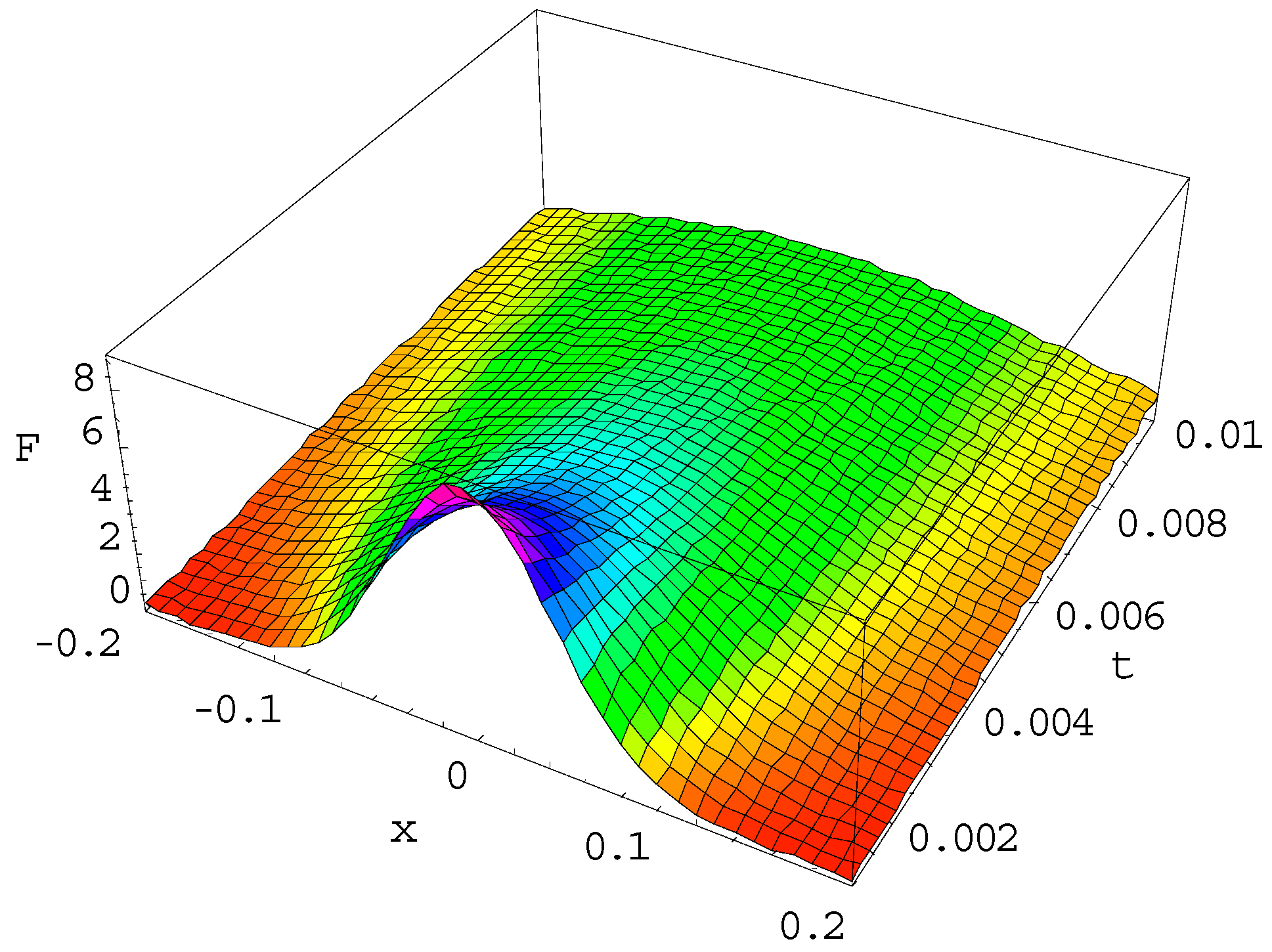
Figure 2.
Solution of the Cattaneo heat equation for μ = 0, α = 1, ε = 1 for the initial function .

Figure 3.
Solution of the Cattaneo heat equation for μ = 0, α = 5, ε = 5 for the initial function .

Figure 4.
Solution F(x, t) of hyperbolic heat equation with initial δ(x) function for α = 100, ε = 10, κ = 1 in the moments of time t = 0.01 (light blue line), t = 0.1 (lilac line), t = 0.3 (pink line), t = 0.6 (blue line) and t = 1.1 (yellow–green line).
Figure 4.
Solution F(x, t) of hyperbolic heat equation with initial δ(x) function for α = 100, ε = 10, κ = 1 in the moments of time t = 0.01 (light blue line), t = 0.1 (lilac line), t = 0.3 (pink line), t = 0.6 (blue line) and t = 1.1 (yellow–green line).

Figure 5.
Schematic diagram of an electric cable line with leakage.

Figure 6.
Space-time distribution of for harmonic for RC = 7, C = L = RL = 1.
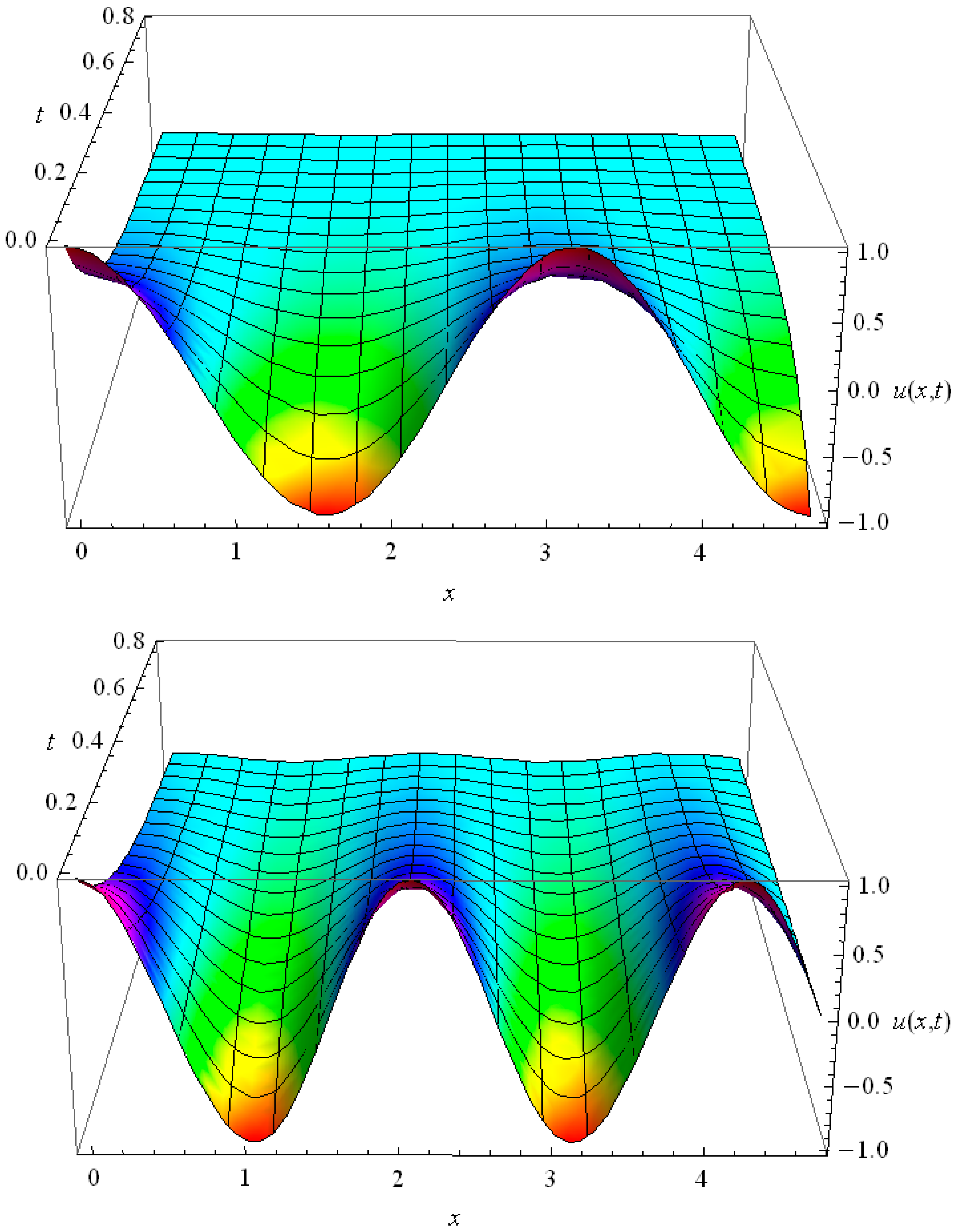
Figure 7.
Space—time distribution of for harmonic for RC = 7, C = L = RL = 1.

Figure 8.
Solution of the Guyer-Krumhansl equation with initial δ(x) function for α = ε = δ = κ = 1 in the interval of time .
Figure 8.
Solution of the Guyer-Krumhansl equation with initial δ(x) function for α = ε = δ = κ = 1 in the interval of time .
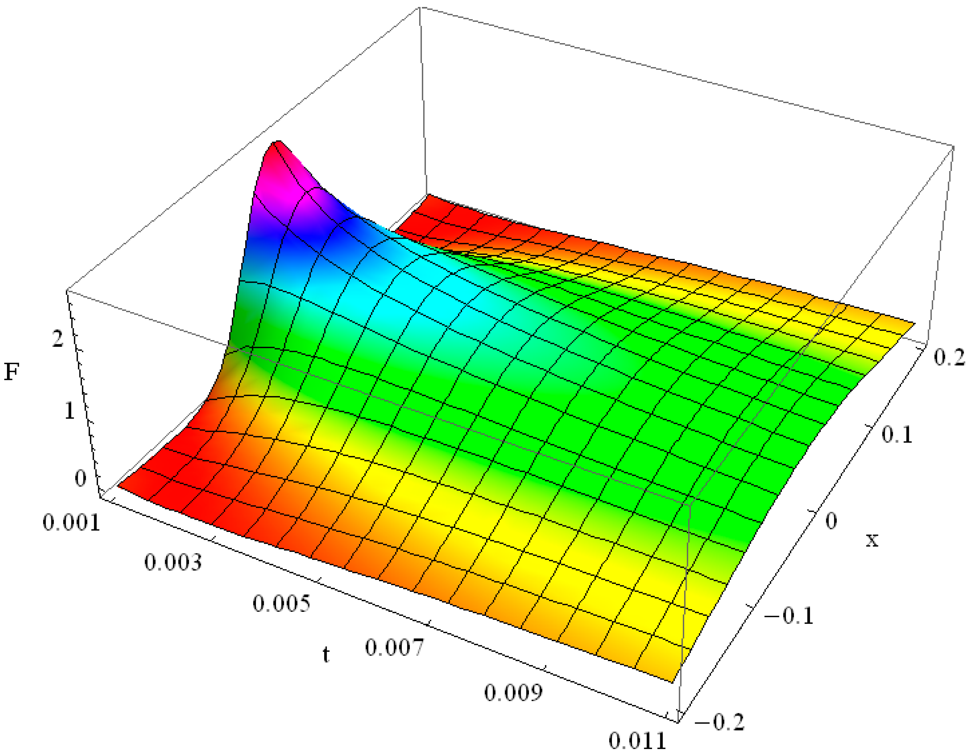
Figure 9.
Heat pulse propagation in the Guyer-Krumhansl model with Knudsen number Kn = 1.

Figure 10.
Heat pulse propagation in the Guyer-Krumhansl (GK) model with Knudsen number Kn = 0.2.
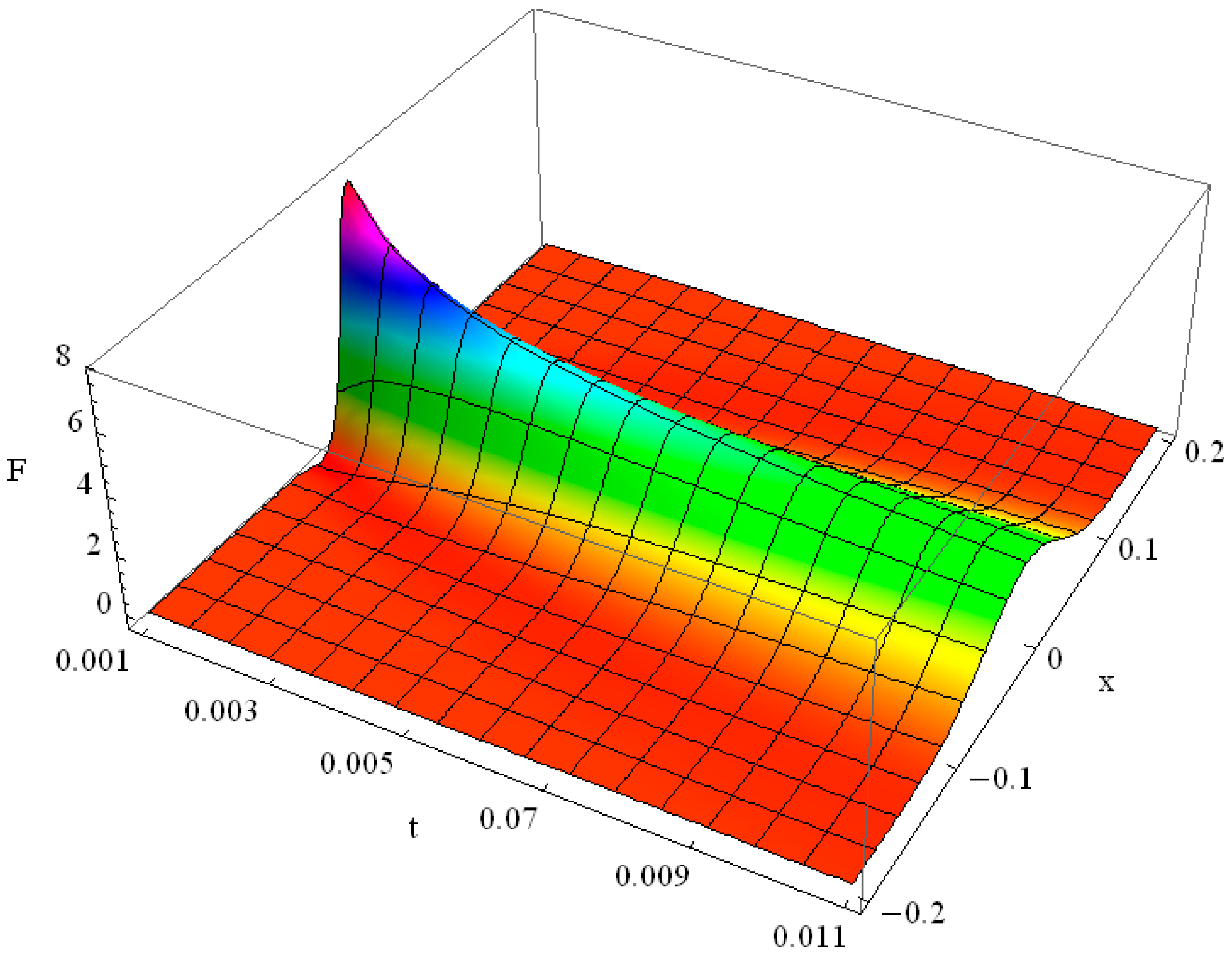
Figure 11.
Solution of GK type equation for heat transport in thin films with Knudsen number Kn = 0.2 for the initial function .
Figure 11.
Solution of GK type equation for heat transport in thin films with Knudsen number Kn = 0.2 for the initial function .
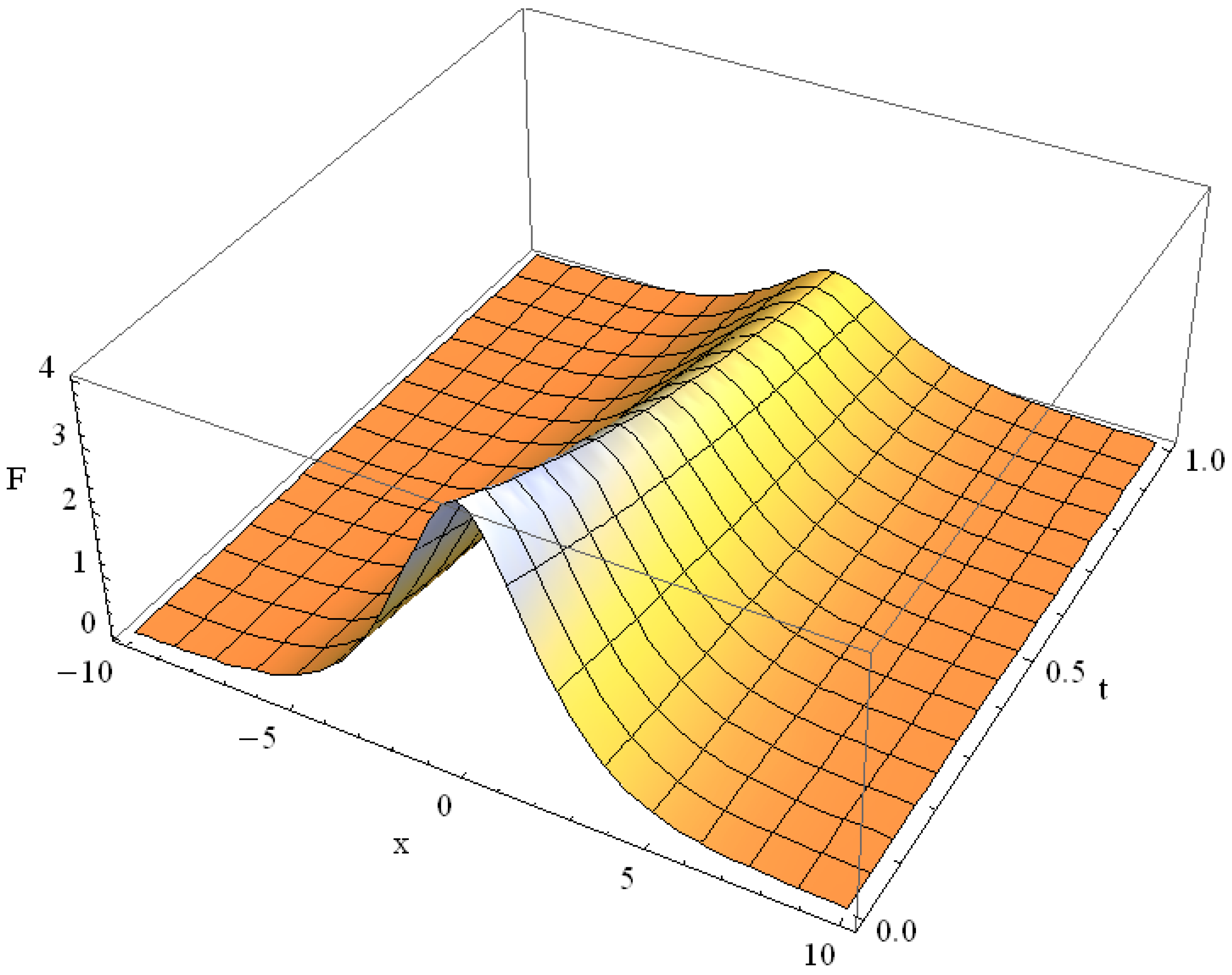
Figure 12.
Solution of GK equation with distinct ballistic transport: α = ε = δ = 10, κ = 0 for the initial function .
Figure 12.
Solution of GK equation with distinct ballistic transport: α = ε = δ = 10, κ = 0 for the initial function .
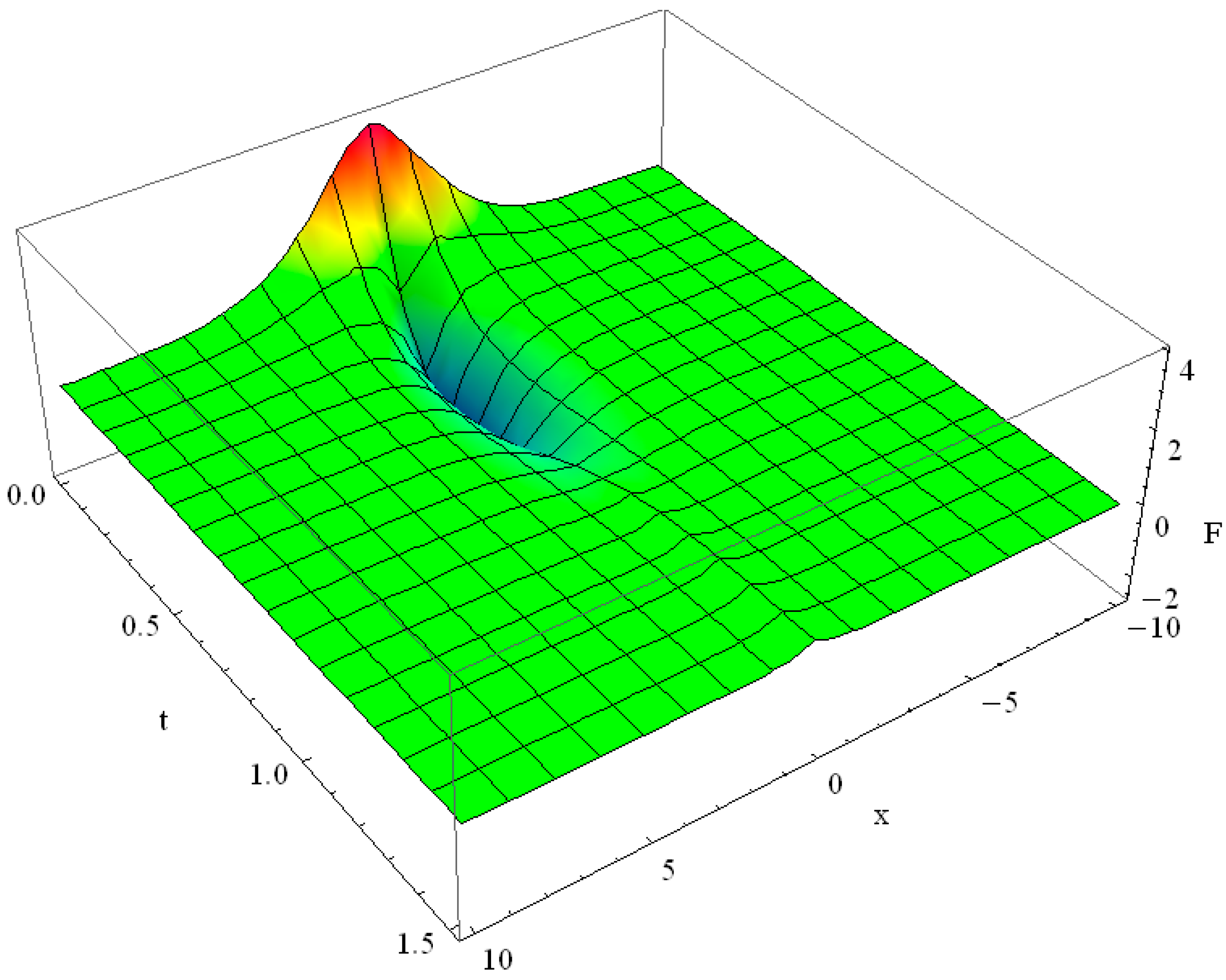
Figure 13.
Solution of GK type Equation: for for (n = 3) left, and for (n = 5) right.
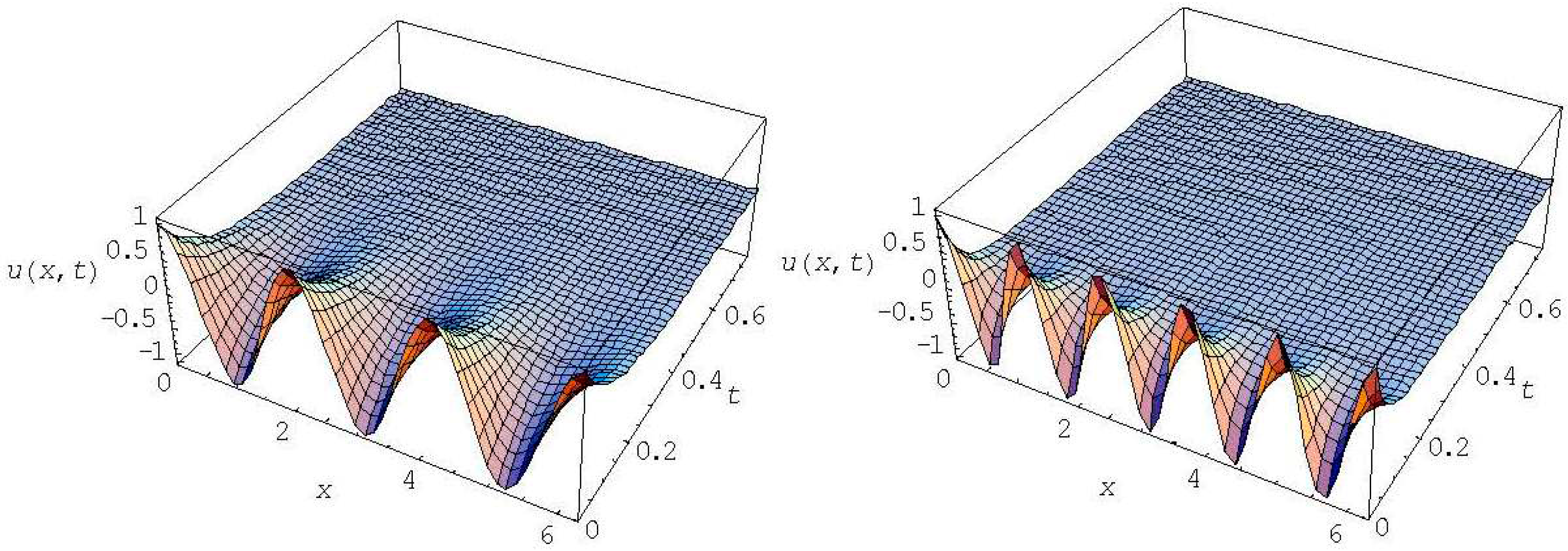
Figure 14.
The behavior of the 1st harmonic (n = 1) of the GK type Equation (36) solution for Kn = 1.
Figure 14.
The behavior of the 1st harmonic (n = 1) of the GK type Equation (36) solution for Kn = 1.
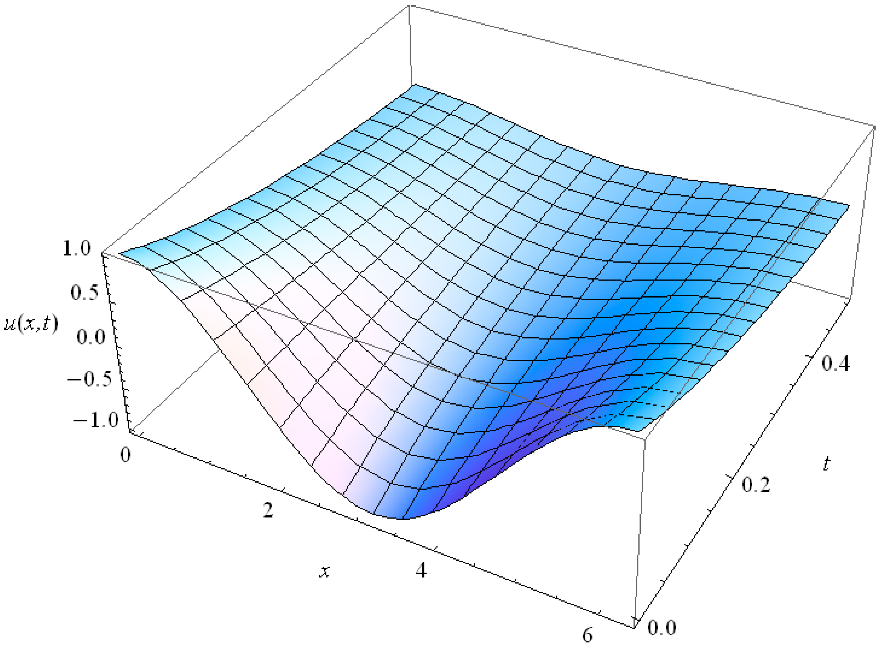
Figure 15.
The behavior of the 3rd harmonic (n = 3) of the GK type Equation (36) solution for Kn = 1.
Figure 15.
The behavior of the 3rd harmonic (n = 3) of the GK type Equation (36) solution for Kn = 1.

Figure 16.
The behavior of the 1st harmonic (n = 1) of the GK type Equation (36) solution for Kn = 0.2.
Figure 16.
The behavior of the 1st harmonic (n = 1) of the GK type Equation (36) solution for Kn = 0.2.
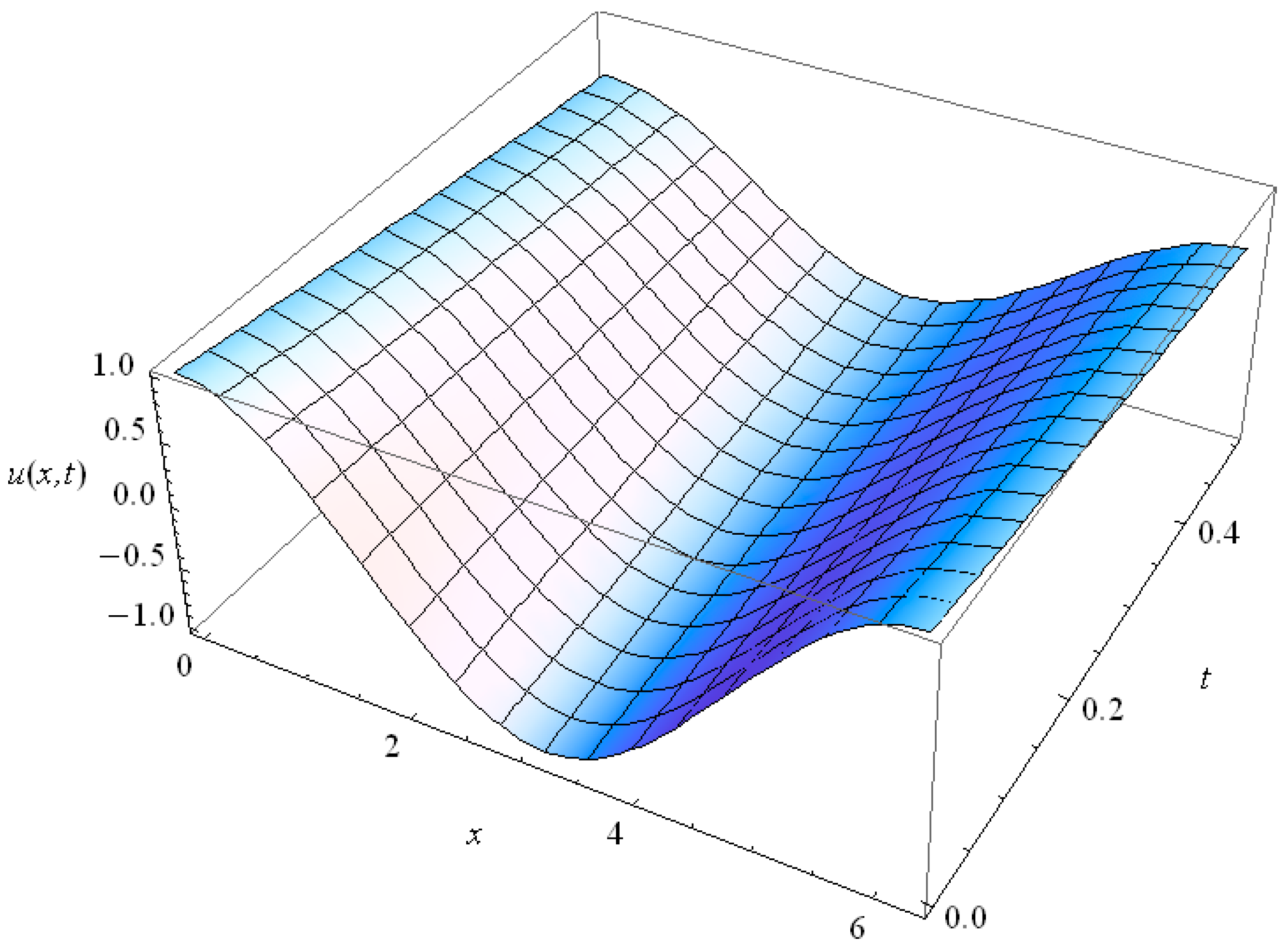
Figure 17.
The behavior of the 3rd harmonic (n = 3) of the GK type Equation (36) solution for Kn = 0.2.
Figure 17.
The behavior of the 3rd harmonic (n = 3) of the GK type Equation (36) solution for Kn = 0.2.

© 2016 by the author; licensee MDPI, Basel, Switzerland. This article is an open access article distributed under the terms and conditions of the Creative Commons Attribution (CC-BY) license (http://creativecommons.org/licenses/by/4.0/).
Share and Cite
MDPI and ACS Style
Zhukovsky, K. Operational Approach and Solutions of Hyperbolic Heat Conduction Equations. Axioms 2016, 5, 28. https://doi.org/10.3390/axioms5040028
AMA Style
Zhukovsky K. Operational Approach and Solutions of Hyperbolic Heat Conduction Equations. Axioms. 2016; 5(4):28. https://doi.org/10.3390/axioms5040028
Chicago/Turabian StyleZhukovsky, Konstantin. 2016. "Operational Approach and Solutions of Hyperbolic Heat Conduction Equations" Axioms 5, no. 4: 28. https://doi.org/10.3390/axioms5040028
Note that from the first issue of 2016, this journal uses article numbers instead of page numbers. See further details here.