Sparse Wavelet Representation of Differential Operators with Piecewise Polynomial Coefficients

Abstract

We propose a construction of a Hermite cubic spline-wavelet basis on the interval and hypercube. The basis is adapted to homogeneous Dirichlet boundary conditions. The wavelets are orthogonal to piecewise polynomials of degree at most seven on a uniform grid. Therefore, the wavelets have eight vanishing moments, and the matrices arising from discretization of differential equations with coefficients that are piecewise polynomials of degree at most four on uniform grids are sparse. Numerical examples demonstrate the efficiency of an adaptive wavelet method with the constructed wavelet basis for solving the one-dimensional elliptic equation and the two-dimensional Black–Scholes equation with a quadratic volatility.

1. Introduction

Wavelets are a powerful and useful tool for analyzing signals, the detection of singularities, data compression and the numerical solution of partial differential and integral equations. One of the most important properties of wavelets is that they have vanishing moments. Vanishing wavelet moments ensure the so-called compression property of wavelets. This means that a function f that is smooth, except at some isolated singularities, typically has a sparse representation in a wavelet basis, i.e., only a small number of wavelet coefficients carry most of the information on f. Similarly as functions, also certain differential and integral operators have sparse or quasi-sparse representation in a wavelet basis. This compression property of wavelets leads to the design of many multiscale wavelet-based methods for the solution of differential equations. The first wavelet methods used orthogonal wavelets, e.g., Daubechies wavelets or coiflets [1,2]. Their disadvantage is that the most orthogonal wavelets are usually not known in a closed form and that their smoothness is typically dependent on the length of the support. The orthogonal wavelets that are known in a closed form are Haar wavelets. They were successfully used for solving differential equations, e.g., in [3,4,5]. Another useful tool is the short Haar wavelet transform that was derived and used for solving differential equations in [6,7,8]. Since spline wavelets are known in a closed form and they are smoother and have more vanishing moments than orthogonal wavelets of the same length of support, many wavelet methods using spline wavelets were proposed [9,10,11]. For a review of wavelet methods for solving differential equations, see also [12,13].

It is known that spectral methods can be used to study singularity formation for PDE solution [14,15,16]. Due to their compression property, wavelets can also be used to study singularity formation for PDE solutions. The wavelet approach simply insists on analyzing wavelet coefficients that are large in regions where the singularity occurs and very small in regions where the function is smooth and derivatives are relatively small. Many adaptive wavelet methods are based on this property [17,18].

We focus on an adaptive wavelet method that was originally designed in [17,18] and later modified in many papers [19,20,21], because it has the following advantages:

• Optimality: For a large class of differential equations, both linear and nonlinear, it was shown that this method converges and is asymptotically optimal in the sense that the storage and number of floating point operations, needed to resolve the problem with desired accuracy, depend linearly on the number of parameters representing the solution, and the number of these parameters is small. Thus, the computational complexity for all steps of the algorithm is controlled.
• High order-approximation: The method enables high order approximation. The order of approximation depends on the order of the spline wavelet basis.
• Sparsity: The solutions and the right-hand side of the equation have sparse representation in a wavelet basis, i.e., they are represented by a small number of numerically significant parameters. In the beginning, iterations start for a small vector of parameters, and the size of the vector increases successively until the required tolerance is reached. The differential operator is represented by a sparse or quasi-sparse matrix, and a procedure for computing the product of this matrix with a finite-length vector with linear complexity is known.
• Preconditioning: For a large class of problems, the matrices arising from a discretization using wavelet bases can be simply preconditioned by a diagonal preconditioner, and the condition numbers of these preconditioned matrices are uniformly bounded. It is important that the preconditioner is simple, such as the diagonal preconditioner, because in some implementations, only nonzero elements in columns of matrices corresponding to significant coefficients of solutions are stored and used.

It should be noted that also other spline wavelet methods utilize some of these features, but to our knowledge, there are no other wavelet methods than adaptive wavelet methods based on the ideas from [17,18] that have all of these properties. For more details about adaptive wavelet methods, see Section 6 and [17,18,19,20,21,22,23].

In this paper, we are concerned with the wavelet discretization of the partial differential equation:

$$-{\displaystyle \sum _{k,l=1}^d}\frac{\partial }{\partial x_k}\left(p_{k,l}\frac{\partial u}{\partial x_l}\right)+{\displaystyle \sum _{k=1}^d}{q}_k\frac{\partial u}{\partial x_k}+p_{0}u=f\mathrm{on}\Omega ={\left(0,1\right)}^d,u=0\mathrm{on}\partial \Omega .$$

(1)

We assume that $q_k\left(x\right)\ge Q>0$, that the functions $p_{k,l}$, $q_k$, $p_0$ and f are sufficiently smooth and bounded on Ω and that $p_{k,l}$ satisfy the uniform ellipticity condition:

$${\displaystyle \sum _{k=1}^d}{\displaystyle \sum _{l=1}^d}{p}_{k,l}\left(x\right)x_k{x}_l\ge C{\displaystyle \sum _{k=1}^d}{x}_k^2,x=\left(x_1,\dots ,x_d\right),$$

(2)

where $C>0$ is independent of x. The discretization matrix for wavelet bases is typically not sparse, but only quasi-sparse, i.e., the matrix of the size $N\times N$ has $\mathcal{O}\left(N\times \log N\right)$ nonzero entries. For multiplication of this matrix with a vector, a routine called APPLYhas to be used [18,19,24]. However, it was observed in several papers, e.g., in [25], that “quantitatively the application of the APPLY routine is very demanding, where this routine is also not easy to implement”. Therefore, in [25] a wavelet basis was constructed with respect to which the discretization matrix is sparse, i.e., it has $\mathcal{O}\left(N\right)$ nonzero entries, for Equation (1) if the coefficients are constant. The construction from [25] was modified in [26,27] with the aim to improve the condition number of the discretization matrices. Some numerical experiments with these bases can be found in [28,29]. In this paper, our aim is to construct a wavelet basis such that the discretization matrix corresponding to (1) is sparse if the coefficients $p_{k,l}$, $q_k$ and $p_0$ are piecewise polynomial functions of degree at most n on the uniform grid, where $n=6$ for $p_{k,l}$, $n=5$ for $q_k$ and $n=4$ for $p_0$. Our construction is based on Hermite cubic splines. Let us mention that cubic Hermite wavelets were constructed also in [25,26,27,30,31,32,33,34,35].

Example 1.

We have recently implemented the adaptive wavelet method for solving the Black–Scholes equation:

$$\frac{\partial V}{\partial t}-{\displaystyle \sum _{k,l=1}^d}\frac{{\rho }_{k,l}}{2}{\sigma }_k{\sigma }_l{S}_k{S}_l\frac{{\partial }^{2}V}{\partial S_k\partial S_l}-r{\displaystyle \sum _{k=1}^d}{S}_k\frac{\partial V}{\partial S_k}+rV=0,$$

(3)

where $\left(S_1,\dots ,S_d,t\right)\in \left(0,S_1^{max}\right)\times \dots \times \left(0,S_d^{max}\right)\times \left(0,T\right)$. We used the θ-scheme for time discretization and tested the performance of the adaptive method with respect to the choice of a wavelet basis for $d=1,2,3$. Some results can be found in [28]. In the case of cubic spline wavelets, the smallest number of iterations was required for the wavelet basis from [36]. The discretization matrix for most spline wavelet bases is not sparse, but only quasi-sparse, and thus, the above-mentioned routine APPLY has to be used. For wavelet bases from [25,26,27], the discretization matrix corresponding to the Black–Scholes operator is sparse if volatilities ${\sigma }_i$ are constant. However, in more realistic models, volatilities are represented by non-constant functions, e.g., piecewise polynomial functions [37]. For the basis that will be constructed in this paper, the discretization matrix is sparse also for the Black–Scholes equation with volatilities ${\sigma }_i$ that are piecewise quadratic.

2. Wavelet Bases

In this section, we briefly review the concept of a wavelet basis in Sobolev spaces and introduce notations; for more details, see, e.g., [23]. Let H be a Hilbert space with the inner product ${〈·,·〉}_H$ and the norm ${∥·∥}_H$, and let $〈·,·〉$ denote the $L^2$-inner product. Let $\mathcal{J}$ be an index set, and let each index $\lambda \in \mathcal{J}$ take the form $\lambda =\left(j,k\right)$, where $\left|\lambda \right|:=j\in \mathbb{Z}$ is a level. For $\mathbf{v}={\left\{v_{\lambda }\right\}}_{\lambda \in \mathcal{J}}$, $v_{\lambda }\in \mathbb{R}$, we define:

$${∥\mathbf{v}∥}_2:={\left(\sum _{\lambda \in \mathcal{J}}{\left|v_{\lambda }\right|}^2\right)}^{1/2},l^2\left(\mathcal{J}\right):=\left\{\mathbf{v}:{∥\mathbf{v}∥}_2<\infty \right\}.$$

(4)

Our aim is to construct a wavelet basis in the sense of the following definition.

Definition 1.

A family $\Psi :=\left\{{\psi }_{\lambda },\lambda \in \mathcal{J}\right\}$ is called a wavelet basis of H, if:

(i) 

Ψ is a Riesz basis for H, i.e., the closure of the span of Ψ is H, and there exist constants $c,C\in \left(0,\infty \right)$, such that:

$$c{∥\mathbf{b}∥}_2\le {∥\sum _{\lambda \in \mathcal{J}}{b}_{\lambda }{\psi }_{\lambda }∥}_H\le C{∥\mathbf{b}∥}_2,\mathit{for}\mathit{all}\mathbf{b}:={\left\{b_{\lambda }\right\}}_{\lambda \in \mathcal{J}}\in l^2\left(\mathcal{J}\right).$$

(5)

(ii) 

The functions are local in the sense that $\mathrm{diam}\left(\mathrm{supp}{\psi }_{\lambda }\right)\le \tilde{C}{2}^{-\left|\lambda \right|}$ for all $\lambda \in \mathcal{J}$, and at a given level j, the supports of only finitely many wavelets overlap at any point x.

For the two countable sets of functions $\Gamma ,\tilde{\Gamma }\subset H$, the symbol ${〈\Gamma ,\tilde{\Gamma }〉}_H$ denotes the matrix:

$${〈\Gamma ,\tilde{\Gamma }〉}_H:={\left\{{〈\gamma ,\tilde{\gamma }〉}_H\right\}}_{\gamma \in \Gamma ,\tilde{\gamma }\in \tilde{\Gamma }}.$$

(6)

The constants $c_{\Psi }:=\sup \left\{c:c\mathrm{satisfies}(5)\right\}$ and $C_{\Psi }:=\inf \left\{C:C\mathrm{satisfies}(5)\right\}$ are called Riesz bounds, and the number $cond\Psi =C_{\Psi }/c_{\Psi }$ is called the condition number of Ψ. It is known that:

$$c_{\Psi }=\sqrt{{\lambda }_{min}\left({〈\Psi ,\Psi 〉}_H\right)},C_{\Psi }=\sqrt{{\lambda }_{max}\left({〈\Psi ,\Psi 〉}_H\right)},$$

(7)

where ${\lambda }_{min}\left({〈\Psi ,\Psi 〉}_H\right)$ and ${\lambda }_{max}\left({〈\Psi ,\Psi 〉}_H\right)$ are the smallest and the largest eigenvalues of the matrix ${〈\Psi ,\Psi 〉}_H$, respectively.

Let M be a Lebesgue measurable subset of ${\mathbb{R}}^d$. The space $L^2\left(M\right)$ is the space of all Lebesgue measurable functions on M, such that the norm:

$$∥f∥={\left(\underset{M}{\int }{\left|f\left(x\right)\right|}^{2}dx\right)}^{1/2}$$

(8)

is finite. The space $L^2\left(M\right)$ is a Hilbert space with the inner product:

$$〈f,g〉={\int }_{M}f\left(x\right)\overline{g\left(x\right)}dx,f,g\in L^2\left(M\right).$$

(9)

The Sobolev space $H^s\left({\mathbb{R}}^d\right)$ for $s\ge 0$ is defined as the space of all functions $f\in L^2\left({\mathbb{R}}^d\right)$, such that the seminorm:

$${\left|f\right|}_{H^s\left({\mathbb{R}}^d\right)}={\left(\frac{1}{{\left(2\pi \right)}^d}{\int }_{{\mathbb{R}}^d}{\left|\widehat{f}\left(\xi \right)\right|}^2{\left|\xi \right|}^{2s}d\xi \right)}^{1/2}$$

(10)

is finite. The symbol $\widehat{f}$ denotes the Fourier transform of the function f defined by:

$$\widehat{f}\left(\xi \right)={\int }_{{\mathbb{R}}^s}f\left(x\right)e^{-i\xi ·x}dx.$$

(11)

The space $H^s\left({\mathbb{R}}^d\right)$ is a Hilbert space with the inner product:

$${〈f,g〉}_{H^s\left({\mathbb{R}}^d\right)}=\frac{1}{{\left(2\pi \right)}^d}{\int }_{{\mathbb{R}}^d}\widehat{f}\left(\xi \right)\overline{\widehat{g}\left(\xi \right)}\left(1+{\left|\xi \right|}^{2s}\right)d\xi ,f,g\in H^s\left({\mathbb{R}}^d\right),$$

(12)

and the norm:

$${∥f∥}_{H^s\left({\mathbb{R}}^d\right)}=\sqrt{{〈f,f〉}_{H^s\left({\mathbb{R}}^d\right)}}.$$

(13)

For an open set $M\subset {\mathbb{R}}^d$, $H^s\left(M\right)$ is the set of restrictions of functions from $H^s\left({\mathbb{R}}^d\right)$ to M equipped with the norm:

$${∥f∥}_{H^s\left(M\right)}=\inf \left\{{∥g∥}_{H^s\left({\mathbb{R}}^d\right)}:g\in H^s\left(M\right){\mathrm{and}g|}_M=f\right\}.$$

(14)

Let $C_0^{\infty }\left(M\right)$ be the space of all continuous functions with the support in M, such that they have continuous derivatives of order r for any $r\in \mathbb{R}$. The space $H_0^s\left(M\right)$ is defined as the closure of $C_0^{\infty }\left(M\right)$ in $H^s\left({\mathbb{R}}^d\right)$. It is known that:

$${∥f∥}_{H^1\left(M\right)}={\left|f\right|}_{H^1\left(M\right)}+∥f∥,$$

(15)

where:

$${\left|f\right|}_{H^1\left(M\right)}=\sqrt{〈\nabla f,\nabla f〉}$$

(16)

is the seminorm in $H^1\left(M\right)$ and $\nabla f$ denotes the gradient of f.

3. Construction of Scaling Functions

We start with the same scaling functions as in [25,26,27,30,31,32,33,34]. Let:

$${\varphi }_1(x)=\left\{\begin{array}{cc}{\left(x+1\right)}^2\left(1-2x\right),& x\in [-1,0],\hfill \\ {\left(1-x\right)}^2\left(1+2x\right),& x\in [0,1],\hfill \\ 0,& \mathrm{otherwise},\hfill \end{array}\right.{\varphi }_2(x)=\left\{\begin{array}{cc}{\left(x+1\right)}^{2}x,& x\in [-1,0],\hfill \\ {\left(1-x\right)}^{2}x,& x\in [0,1],\hfill \\ 0,& \mathrm{otherwise}.\hfill \end{array}\right.$$

(17)

For $j\ge 3$ and $x\in \left[0,1\right]$, we define:

$$\begin{array}{c}{\varphi }_{j,2k+l-1}\left(x\right)=2^{j/2}{\varphi }_l\left(2^{j}x-k\right)\mathrm{for}k=1,\dots ,2^j-1,l=1,2,\\ {\varphi }_{j,1}\left(x\right)=2^{j/2}{\varphi }_2\left(2^{j}x\right),{\varphi }_{j,2^{j+1}}\left(x\right)=2^{j/2}{\varphi }_2\left(2^j\left(x-1\right)\right),\end{array}$$

(18)

and:

$${\Phi }_j=\left\{{\varphi }_{j,k},k=1,\dots ,2^{j+1}\right\},V_j=\mathrm{span}{\Phi }_j.$$

(19)

The scaling functions ${\varphi }_{j,k}$ on the level $j=3$ are displayed in Figure 1.

Then, the spaces $V_j$ form a multiresolution analysis. We choose dual space ${\tilde{V}}_j$ as the set of all functions $v\in L^2\left(0,1\right)$, such that v restricted to the interval $\left(\frac{k-1}{2^{j-2}},\frac{k}{2^{j-2}}\right)$ is a polynomial of degree less than eight for any $k=1,\dots ,2^{j-2}$, i.e.,

$${\tilde{V}}_j=\left\{v\in L^2\left(0,1\right){:v|}_{\left(\frac{k-1}{2^{j-2}},\frac{k}{2^{j-2}}\right)}\in {\mathrm{\Pi }}_8\left(\frac{k-1}{2^{j-2}},\frac{k}{2^{j-2}}\right)\mathrm{for}k=0,\dots ,2^{j-2}\right\},$$

(20)

where ${\mathrm{\Pi }}_8\left(a,b\right)$ denotes the set of all polynomials on $\left(a,b\right)$ of degree less than eight. Let:

$$W_j={\tilde{V}}_j^{\perp }\cap V_{j+1},$$

(21)

where ${\tilde{V}}_j^{\perp }$ is the orthogonal complement of ${\tilde{V}}_j$ with respect to the $L^2$-inner product. If a function g is a piecewise polynomial of degree n, we write $\mathrm{deg}g=n$.

Lemma 1.

Let the spaces $W_j$, $j\ge 3$, be defined as above. Then, all functions $g\in W_i$ and $h\in W_j$, $i,j\ge 3$, $\left|i-j\right|>2$, satisfy:

$$〈ag,h〉=0,〈b{g}^{\prime },h〉=0,〈c{g}^{\prime },h^{\prime }〉=0,$$

(22)

where $a,b,c$ are piecewise polynomial functions, such that $a,b,c\in {\tilde{V}}_p$, $p\le \max \left(i,j\right)$, $\mathrm{deg}a\le 4$, $\mathrm{deg}b\le 5$ and $\mathrm{deg}c\le 6$.

Proof of Lemma 2.

Let us assume that $j>i+2$. We have $g\in W_i\subset V_{i+1}\subset V_{j-2}\subset {\tilde{V}}_j$, $\mathrm{deg}g\le 3$, $a\in {\tilde{V}}_j$, $\mathrm{deg}a\le 4$, and thus, $ag\in {\tilde{V}}_j$. Since $h\in W_j$ and $W_j$ is orthogonal to ${\tilde{V}}_j$, we obtain $〈ag,h〉=0$. Similarly, the relation $〈b{g}^{\prime },h〉=0$ is the consequence of the fact that $b{g}^{\prime }\in {\tilde{V}}_j$ and $h\in W_j$. Using integration by parts, we obtain:

$$〈c{g}^{\prime },h^{\prime }〉=-〈c^{\prime }{g}^{\prime }+c{g}^{″},h〉.$$

(23)

Since $c^{\prime }{g}^{\prime }+c{g}^{″}\in {\tilde{V}}_j$ and $h\in W_j$, we have $〈c{g}^{\prime },h^{\prime }〉=0$. The situation for $j<i+2$ is similar. ☐

Therefore, the discretization matrix for the Equation (1) is sparse. Let ${\Psi }_j$ be a basis of $W_j$. The proof that:

$$\Psi =\left\{{\psi }_{\lambda },\lambda \in \mathcal{J}\right\}={\Phi }_3\cup {\displaystyle \bigcup _{j=3}^{\infty }}{\Psi }_j.$$

(24)

is a Riesz basis of the space $L^2\left(0,1\right)$, and that Ψ is a Riesz basis of the space $H_0^1\left(0,1\right)$ when normalized with respect to the $H^1$-norm is based on the following theorem [25,38].

Theorem 2.

Let $J\in \mathbb{N}$, and let $V_j$ and ${\tilde{V}}_j$, $j\ge J$, be subspaces of $L^2\left(0,1\right)$, such that:

$$V_j\subset V_{j+1},{\tilde{V}}_j\subset {\tilde{V}}_{j+1},\dim V_j=\dim {\tilde{V}}_j<\infty ,j\ge J.$$

(25)

Let ${\Phi }_j$ be bases of $V_j$, ${\tilde{\Phi }}_j$ be bases of ${\tilde{V}}_j$ and ${\Psi }_j$ be bases of ${\tilde{V}}_j^{\perp }\cap V_{j+1}$, such that Riesz bounds with respect to the $L^2$-norm of ${\Phi }_j$; ${\tilde{\Phi }}_j$, and ${\Psi }_j$ are uniformly bounded; and let Ψ be given by (24). Furthermore, let the matrix:

$${\mathbf{G}}_j:=〈{\Phi }_j,{\tilde{\Phi }}_j〉$$

(26)

be invertible, and the spectral norm of ${\mathbf{G}}_j^{-1}$ is bounded independently of j. In addition, for some positive constants C, γ and d, such that $\gamma <d$, let:

$$\underset{v_j\in V_j}{\inf }∥v-v_j∥\le C{2}^{-jd}{∥v∥}_{H^d\left(0,1\right)},v\in H_0^d\left(0,1\right),$$

(27)

and for $0\le s<\gamma$, let:

$${∥v_j∥}_{H^d\left(0,1\right)}\le C{2}^{js}∥v_j∥,v_j\in V_j;$$

(28)

and let similar estimates (27) and (28) hold for $\tilde{\gamma }$ and $\tilde{d}$ on the dual side. Then, there exist constants k and K, $0<k\le K<\infty$, such that:

$$k{∥\mathbf{b}∥}_2\le {∥\sum _{\lambda \in \mathcal{J}}{b}_{\lambda }{2}^{-\left|\lambda \right|s}{\psi }_{\lambda }∥}_{H^s\left(0,1\right)}\le K{∥\mathbf{b}∥}_2,\mathbf{b}:={\left\{b_{\lambda }\right\}}_{\lambda \in \mathcal{J}}\in l^2\left(\mathcal{J}\right)$$

(29)

holds for $s\in \left(-\tilde{\gamma },\gamma \right)$.

We focus on the spaces $V_j$ and ${\tilde{V}}_j$ defined by (19) and (20), respectively, and we show that they satisfy the assumptions of Theorem 2.

Theorem 3.

There exist uniform Riesz bases ${\widehat{\Phi }}_j$ of $V_j$ and ${\tilde{\Phi }}_j$ of ${\tilde{V}}_j$, such that the matrix:

$${\mathbf{G}}_j=〈{\widehat{\Phi }}_j,{\tilde{\Phi }}_j〉$$

(30)

is invertible and the spectral norm of ${\mathbf{G}}_j^{-1}$ is bounded independently of j.

Proof of Theorem 4.

Let ${\Phi }_j$, $V_j$ and ${\tilde{V}}_j$ be defined as above. For $i=0,\dots ,7$, we define:

$$p_i\left(x\right)\left\{\begin{array}{cc}{\left(x-1/2\right)}^i,& x\in \left[0,1\right],\hfill \\ 0,& \mathrm{otherwise},\hfill \end{array}\right.$$

(31)

and:

$${\theta }_{j,8k+i+1}=2^{\left(j-2\right)/2}{p}_i\left(2^{j-2}x-k\right),k\in \mathbb{Z},i=0,\dots ,7.$$

(32)

Then, the set ${\Theta }_j=\left\{{\theta }_{j,k},k=1,\dots ,2^{j+1}\right\}$ is a basis of ${\tilde{V}}_j$, and the matrix ${\mathbf{A}}_j=〈{\Phi }_j,{\Theta }_j〉$, $j\ge 3$, has the structure:

(33)

where $\mathbf{A}$ is the matrix of the size $10\times 8$. Our aim is to apply several transforms on ${\Phi }_j$ and ${\Theta }_j$, such that new bases ${\widehat{\Phi }}_j$ of $V_j$ and ${\tilde{\Phi }}_j$ of ${\tilde{V}}_j$ are local, and the matrix ${\mathbf{G}}_j$ defined by (30) and its transpose ${\mathbf{G}}_j^T$ are both strictly diagonally dominant. First, we replace functions ${\theta }_{j,k}$ by functions $g_{j,k}$ in such a way that the matrix of $L^2$-inner products of ${\varphi }_{j,k}$ and $g_{j,l}$ is tridiagonal. Therefore, we define:

$$g_{j,8k+i+1}={\displaystyle \sum _{l=1}^8}{c}_{j,l}^i{\theta }_{j,8k+l},i=0,\dots ,7,k=0,\dots ,2^{j-2}-1,$$

(34)

where the coefficients $c_{j,l}^i$ are chosen, such that:

$$〈{\varphi }_{j,p},g_{j,q}〉=0,\left|p-q\right|>1,〈{\varphi }_{j,p},g_{j,p}〉=1,p=1,\dots ,2^{j+1}-1.$$

(35)

For $m=8k+i+1$, $i=0,\dots ,7$, $k=1,\dots ,2^{j-2}-2$, we substitute (34) into (35), and using $\mathrm{supp}{\varphi }_{j,8k+l+1}\cap \mathrm{supp}{g}_{j,m}=0$ for $l\ne 0,\dots ,9$, we obtain systems of eight linear algebraic equations with eight unknown coefficients:

$${\mathbf{A}}^i{\mathbf{c}}^i={\mathbf{e}}^i,\mathrm{for}k=2,\dots ,2^{j-2}-2,{\mathbf{c}}^i={\left(c_{j,l}^i\right)}_{l=1}^8,$$

(36)

the system matrices ${\mathbf{A}}^i$ that are submatrices of $\mathbf{A}$ containing all rows of $\mathbf{A}$ except the i-th and $\left(i+2\right)$-th rows, and ${\mathbf{e}}^i$ are unit vectors, such that ${\left({\mathbf{e}}^i\right)}_l={\delta }_{i,l}$. The symbol ${\delta }_{i,l}$ denotes the Kronecker delta. We computed all of the system matrices precisely using symbolic computations and verified that they are regular. Thus, the coefficients $c_{j,l}^i$ exist and are unique.

The matrix ${\mathbf{B}}_j$ defined by ${\left({\mathbf{B}}_j\right)}_{k,l}=〈{\varphi }_{j,k},g_{j,m}〉$, $k,l=1,\dots ,2^{j+1},$ is tridiagonal and has the structure:

(37)

where:

$$\mathbf{B}=\left(\begin{array}{cccccccc}\hfill 13.199& \hfill 0& \hfill 0& \hfill 0& \hfill 0& \hfill 0& \hfill 0& \hfill 0\\ \hfill 1.000& \hfill 0.098& \hfill 0& \hfill 0& \hfill 0& \hfill 0& \hfill 0& \hfill 0\\ \hfill -2.185& \hfill 1.000& \hfill -24.781& \hfill 0& \hfill 0& \hfill 0& \hfill 0& \hfill 0\\ \hfill 0& \hfill -0.138& \hfill 1.000& \hfill 0.104& \hfill 0& \hfill 0& \hfill 0& \hfill 0\\ \hfill 0& \hfill 0& \hfill 13.887& \hfill 1.000& \hfill -6.026& \hfill 0& \hfill 0& \hfill 0\\ \hfill 0& \hfill 0& \hfill 0& \hfill -0.074& \hfill 1.000& \hfill 0.041& \hfill 0& \hfill 0\\ \hfill 0& \hfill 0& \hfill 0& \hfill 0& \hfill 34.953& \hfill 1.000& \hfill 8.824& \hfill 0\\ \hfill 0& \hfill 0& \hfill 0& \hfill 0& \hfill 0& \hfill -0.018& \hfill 1.000& \hfill 0.023\\ \hfill 0& \hfill 0& \hfill 0& \hfill 0& \hfill 0& \hfill 0& \hfill -9.423& \hfill 1.000\\ \hfill 0& \hfill 0& \hfill 0& \hfill 0& \hfill 0& \hfill 0& \hfill 0& \hfill -0.092\end{array}\right),$$

(38)

and:

$${\mathbf{B}}^L={\mathbf{B}}_{\left\{2,\dots ,10\right\}},{\mathbf{B}}^R={\mathbf{B}}_{\left\{1,\dots ,8,10\right\}}.$$

(39)

The symbol ${\mathbf{B}}_M$ denotes the submatrix of the matrix $\mathbf{B}$ containing rows from $\mathbf{B}$ with indices from $M$. In (38), the numbers are rounded to three decimal digits.

We apply several transforms on ${\varphi }_{j,k}$ and denote the new functions by ${\varphi }_{j,k}^i$. In the following, let:

$$B_{j,k,l}={\left({\mathbf{B}}_j\right)}_{k,l},B_{j,k,l}^i=〈{\varphi }_{j,l}^i,g_{j,k}〉,i=1,\dots ,4.$$

(40)

We define:

$$\begin{array}{c}{\varphi }_{j,k}^1={\varphi }_{j,k}-\frac{B_{j,k,k+1}}{B_{j,k+1,k+1}}{\varphi }_{j,k+1}\mathrm{for}k\mathrm{even},{\varphi }_{j,k}^1={\varphi }_{j,k}\mathrm{for}k\mathrm{odd},\\ {\varphi }_{j,k}^2={\varphi }_{j,k}^1-\frac{B_{j,k,k-1}^1}{B_{j,k-1,k-1}^1}{\varphi }_{j,k-1}^1\mathrm{for}k\mathrm{even},{\varphi }_{j,k}^2={\varphi }_{j,k}^1\mathrm{for}k\mathrm{odd},\\ {\varphi }_{j,4+8k}^3={\varphi }_{j,4+8k}^2-\frac{B_{j,4+8k,2+8k}^2}{B_{j,2+8k,2+8k}^2}{\varphi }_{j,2+8k}^1\mathrm{for}k=1,\dots ,2^{j-2},{\varphi }_{j,l}^3={\varphi }_{j,l}^2\mathrm{otherwise},\\ {\varphi }_{j,6+8k}^4={\varphi }_{j,6+8k}^3-\frac{B_{j,6+8k,4+8k}^3}{B_{j,4+8k,4+8k}^3}{\varphi }_{j,4+8k}^1\mathrm{for}k=1,\dots ,2^{j-2},{\varphi }_{j,l}^4={\varphi }_{j,l}^3\mathrm{otherwise},\end{array}$$

(41)

and:

$${\widehat{\varphi }}_{j,l}=\left\{\begin{array}{cc}2.1{\varphi }_{j,l}^4\hfill & l=4+8k,\hfill \\ 10{\varphi }_{j,l}^4\hfill & l=2^{j+1},\hfill \\ {\varphi }_{j,l}^4\hfill & \mathrm{otherwise}.\hfill \end{array}\right.$$

(42)

Furthermore, we set ${\tilde{\varphi }}_{j,2+8k}=1.3g_{j,2+8k}$ for $k=0,\dots ,2^{j-2}$ and ${\tilde{\varphi }}_{j,l}=g_{j,l}$ for $l\ne 2+8k$. Let ${\widehat{\Phi }}_j=\left\{{\widehat{\varphi }}_{j,l},l=1,\dots 2^{j+1}\right\}$ and ${\tilde{\Phi }}_j=\left\{{\tilde{\varphi }}_{j,l},l=1,\dots 2^{j+1}\right\}$. The matrix ${\mathbf{G}}_j$ defined by (30) has the same structure as ${\mathbf{A}}_j$ and ${\mathbf{B}}_j$, i.e.,

$$\begin{array}{ccc}\hfill {\left({\mathbf{G}}_j\left(8i+k,8i+l\right)\right)}_{k=0,\dots ,14,l=1,\dots ,8}& =& \mathbf{G},i=2,\dots ,2^{j-2}-2\hfill \\ \hfill {\left({\mathbf{G}}_j\left(k,l\right)\right)}_{k=1,\dots ,14,l=1,\dots ,8}& =& {\mathbf{G}}^L,\hfill \\ \hfill {\left({\mathbf{G}}_j\left(2^{j+1}-8+k,2^{j+1}-8+l\right)\right)}_{k=0,\dots ,8,l=1,\dots ,8}& =& {\mathbf{G}}^R,\hfill \end{array}$$

(43)

where:

$$\mathbf{G}=\left(\begin{array}{cccccccc}0& -1.6863& 0& 0& 0& 0& 0& 0\\ 1.0000& 0.1278& 0& 0& 0& 0& 0& 0\\ 0& -2.8555& 0& 2.5773& 0& 0& 0& 0\\ 0& -0.1790& 1.0000& 0.1040& 0& 0& 0& 0\\ 0& 0& 0& 2.8443& 0& 0.5229& 0& 0\\ 0& 0& 0& -0.0737& 1.0000& 0.0413& 0& 0\\ 0& 0& 0& 0& 0& -0.7599& 0& -0.2011\\ 0& 0& 0& 0& 0& -0.0179& 1.0000& 0.0228\\ 0& 0& 0& 0& 0& -0.1689& 0& 2.4295\\ 0& 0& 0& 0& 0& 0& 0& -0.0920\\ 0& 0& 0& 0& 0& 0& 0& -0.2011\\ 0& 0& 0& 0& 0& 0& 0& 0\\ 0& 0& 0& 0& 0& 0& 0& -0.3675\\ 0& 0& 0& 0& 0& 0& 0& 0\\ 0& 0& 0& 0& 0& 0& 0& 0.3330\end{array}\right)$$

(44)

and:

$${\mathbf{G}}^L={\mathbf{G}}_{\left\{2,\dots ,15\right\}},{\mathbf{G}}^R=\left(\begin{array}{cccc}& & {\mathbf{G}}_{\left\{1,\dots ,8\right\}}& \\ 0& \dots & 0& -0.920\end{array}\right)$$

(45)

Thus, the matrices ${\mathbf{G}}_j$ and ${\mathbf{G}}_j^T$ are diagonally dominant and invertible, and due to Johnson’s lower bound for the smallest singular value [39], we have:

$${\sigma }_{min}\left({\mathbf{G}}_j\right)\ge 0.117,{∥{\mathbf{G}}_j^{-1}∥}_2=\frac{1}{{\sigma }_{min}\left({\mathbf{G}}_j\right)}\le 8.527.$$

(46)

It remains to prove that ${\widehat{\Phi }}_j$ are uniform Riesz bases of $V_j$ and ${\tilde{\Phi }}_j$ are uniform Riesz bases of ${\tilde{V}}_j$. Since ${\widehat{\varphi }}_{j,k}$ are locally supported and there exists M independent of j and k, such that ${∥{\widehat{\varphi }}_{j,k}∥}_{L^2\left(0,1\right)}\le M$, we have:

$${∥\sum _k{c}_{j,k}{\widehat{\varphi }}_{j,k}∥}_{L^2\left(0,1\right)}^2=\sum _k\sum _l{c}_{j,k}{c}_{j,l}{\int }_0^1{\widehat{\varphi }}_{j,k}\left(x\right){\widehat{\varphi }}_{j,l}\left(x\right)dx\le C{∥c∥}_2^2.$$

(47)

and similarly for ${\tilde{\varphi }}_{j,k}$, we have:

$${∥\sum _k{c}_{j,k}{\tilde{\varphi }}_{j,k}∥}_{L^2\left(0,1\right)}^2\le C{∥c∥}_2^2.$$

(48)

By the same argument as in the Proof of Theorem 3.3. in [25], from (47), (48), the invertibility of ${\mathbf{G}}_j$ and (46), we can conclude that ${\widehat{\Phi }}_j$ and ${\tilde{\Phi }}_j$ are uniform Riesz bases of their spans. ☐

4. Construction of Wavelets

Now, we construct a basis ${\Psi }_j$ of the space $W_j={\tilde{V}}_j^{\perp }\cap V_{j+1}$, such that $cond{\Psi }_j\le C$, where C is a constant independent on j, and functions from ${\Psi }_j$ are translations and dilations of some generators. We propose one boundary generator ${\psi }^b$ and functions ${\psi }^i$, $i=1,\dots ,8$, generating inner wavelets, such that the sets:

$${\Psi }_j=\left\{{\psi }_{j,k},k=1,\dots ,2^{j+1}\right\},j\ge 3,$$

(49)

contain functions ${\psi }_{j,k}$ defined for $x\in \left[0,1\right]$ by:

$$\begin{array}{c}{\psi }_{j,1}\left(x\right)=2^{j/2}{\psi }^b\left(2^{j}x\right),{\psi }_{j,2^{j+1}}\left(x\right)=2^{j/2}{\psi }^b\left(2^j\left(1-x\right)\right),\\ {\psi }_{j,8k+l+1}\left(x\right)=2^{j/2}{\psi }^l\left(2^{j}x-4k\right),l=1,\dots 8,1<8k+l+1<2^{j+1}.\end{array}$$

(50)

We denote the scaling functions on the level $j=1$ by:

$${\varphi }_{1,2k+l-2}\left(x\right)=2^{1/2}{\varphi }_l\left(2x-k\right)\mathrm{for}k\in \mathbb{Z},l=1,2,x\in \mathbb{R}.$$

(51)

For $l=1,\dots ,6$, let the functions ${\psi }^l$ have the form:

$${\psi }^l={\displaystyle \sum _{k=1}^{14}}{h}_{l,k}{\varphi }_{1,k}$$

(52)

and be such that ${\psi }^1$, ${\psi }^2$ and ${\psi }^3$ are antisymmetric and ${\psi }^4$, ${\psi }^5$ and ${\psi }^6$ are symmetric. Thus, $\mathrm{supp}{\psi }^l=\left[0,4\right]$ for $l=1,\dots ,6$. Let $p_i$ be polynomials defined by (31). It is clear that if:

$$〈{\psi }^l\left(x\right),p_i\left(\frac{x}{4}\right)〉=0,i=0,\dots ,7,l=1,\dots 6,$$

(53)

then $〈{\psi }^l\left(2^{j}x-k\right),p_i\left(2^{j-2}x-m\right)〉=0,$ for $k,m\in 4\mathbb{Z}$, and thus, $〈{\psi }_{j,8i+l},g〉=0$ for any $g\in {\tilde{V}}_j$, $i=0,\dots ,2^{j-2}-1,$ and $l=1,\dots ,6$. Substituting (52) into (53), we obtain the system of linear algebraic equations with the solution ${\mathbf{h}}^l={\left\{h_{l,k}\right\}}_{k=1}^{14}$ of the form:

$${\mathbf{h}}^l=a_{l,1}{\mathbf{u}}_1+a_{l,2}{\mathbf{u}}_2+a_{l,3}{\mathbf{u}}_3,l=1,2,3,$$

(54)

and:

$${\mathbf{h}}^l=b_{l-3,1}{\mathbf{v}}_1+b_{l-3,2}{\mathbf{v}}_2+b_{l-3,3}{\mathbf{v}}_3,l=4,5,6,$$

(55)

where $a_{l,k}$ and $b_{l,k}$ are chosen real parameters and:

$$\left[{\mathbf{u}}_1,{\mathbf{u}}_2,{\mathbf{u}}_3\right]=\left(\begin{array}{ccc}-\frac{29}{95361}& \frac{120}{31787}& \frac{5716}{31787}\\ 0& 0& 1\\ \frac{592}{95361}& \frac{13477}{95361}& -\frac{56300}{95361}\\ 0& 1& 0\\ \frac{13456}{95361}& -\frac{39892}{95361}& \frac{49671}{31787}\\ 1& 0& 0\\ 0& 0& 0\\ \frac{11708}{4541}& -\frac{26022}{4541}& \frac{116428}{4541}\\ -\frac{13456}{95361}& \frac{39892}{95361}& -\frac{49671}{31787}\\ 1& 0& 0\\ -\frac{592}{95361}& -\frac{13477}{95361}& \frac{56300}{95361}\\ 0& 1& 0\\ \frac{29}{95361}& -\frac{120}{31787}& -\frac{5716}{31787}\\ 0& 0& 1\end{array}\right),\left[{\mathbf{v}}_1,{\mathbf{v}}_2,{\mathbf{v}}_3\right]=\left(\begin{array}{ccc}\frac{11}{10500}& -\frac{17}{2625}& -\frac{1727}{10500}\\ 0& 0& -1\\ -\frac{13}{875}& -\frac{293}{2625}& \frac{1123}{2625}\\ 0& -1& 0\\ -\frac{1}{12}& \frac{5}{21}& -\frac{53}{84}\\ -1& 0& 0\\ \frac{34}{175}& -\frac{6}{25}& \frac{386}{525}\\ 0& 0& 0\\ -\frac{1}{12}& \frac{5}{21}& -\frac{53}{84}\\ 1& 0& 0\\ -\frac{13}{875}& -\frac{293}{2625}& \frac{1123}{2625}\\ 0& 1& 0\\ \frac{11}{10500}& -\frac{17}{2625}& -\frac{1727}{10500}\\ 0& 0& 1\end{array}\right).$$

(56)

For $l\in \left\{7,8\right\}$, let the functions ${\psi }^l$ have the form:

$${\psi }^l={\displaystyle \sum _{k=1}^{28}}{h}_{l,k}{\varphi }_{1,k}.$$

(57)

These functions are uniquely determined by imposing that ${\psi }^7$ is symmetric, ${\psi }^8$ is antisymmetric, both ${\psi }^7$ and ${\psi }^8$ are $L^2$-orthogonal to the functions ${\psi }^l$, $l=1,\dots ,6$, they are normalized with respect to the $L^2$-norm and:

$$〈{\psi }^l\left(x\right),p_i\left(\frac{x}{4}\right)〉=0,\mathrm{for}i=0,\dots ,7.$$

(58)

It remains to construct boundary function ${\psi }^b$. Let:

$${\psi }^b={\displaystyle \sum _{k=0}^{14}}{h}_{b,k}{\varphi }_{1,k}{|}_{\left[0,\infty \right)}.$$

(59)

Substituting (59) into:

$$〈{\psi }^b\left(x\right),p_i\left(\frac{x}{4}\right)〉=0,\mathrm{for}i=0,\dots ,7,$$

(60)

we obtain the system of eight equations for 15 unknown coefficients. The solution ${\mathbf{h}}^b={\left\{h_{b,k}\right\}}_{k=0}^{14}$ is the linear combination of vectors ${\mathbf{w}}_i$ given by:

$$\begin{array}{c}{\mathbf{w}}_1={\left(\frac{150}{83},\frac{1429}{1992},\frac{4509}{664},\frac{74}{249},\frac{2839}{166},-\frac{1897}{1992},\frac{6741}{664},-\frac{53}{249},1,0,0,0,0,0,0\right)}^T,\\ {\mathbf{w}}_l=\left(\begin{array}{c}0\\ {\mathbf{u}}_{l-1}\end{array}\right),l=2,3,4,{\mathbf{w}}_l=\left(\begin{array}{c}0\\ {\mathbf{v}}_{l-4}\end{array}\right),l=5,6,7,\end{array}$$

(61)

i.e.,

$${\mathbf{h}}^b={\displaystyle \sum _{i=1}^7}{d}_i{W}_i,$$

(62)

where $d_i$ are chosen real parameters.

Hence, the set ${\Psi }_j$ depends on the choice of $a_{k,l}$, $b_{k,l}$ and $d_i$. However, it is not true that $cond{\Psi }_j\le C$ for all possible choices of these parameters. Moreover, for some choices, the condition numbers of ${\Psi }_j$ are uniformly bounded, but the condition number of the resulting basis Ψ is large, e.g., ${10}^6$.

Therefore, we optimize the construction to improve the condition number of Ψ. We choose $a_{k,1}$, and then, we set $a_{k,2}$ and $a_{k,3}$, such that $〈{\psi }^i,{\psi }^j〉={\delta }_{i,j}$ for $i,j=1,2,3$, and similarly, we choose $b_{k,1}$ and then set $b_{k,2}$ and $b_{k,3}$, such that $〈{\psi }^i,{\psi }^j〉={\delta }_{i,j}$ for $i,j=4,5,6$. Moreover, the functions ${\psi }^7$ and ${\psi }^8$ are constructed, such that they are orthogonal to ${\psi }^i$ for $i=1,\dots ,6$, and due to the symmetry and antisymmetry, we have $〈{\psi }^i,{\psi }^j〉={\delta }_{i,j}$ for $i=1,2,3$ and $j=4,5,6$ and $〈{\psi }^7,{\psi }^8〉=0$. In summary, ${\psi }^i$ is orthogonal to ${\psi }^j$ with respect to the $L^2$-norm for $i,j=1,\dots 6$, $i\ne j$. To further improve the condition number, we orthogonalize scaling functions on the coarsest level $j=3$, i.e., we determine the set:

$${\Phi }_3^{ort}:={\mathbf{K}}^{-1}{\Phi }_3,\mathbf{K}=〈{\Phi }_3,{\Phi }_3〉,$$

(63)

and we redefine ${\Phi }_3$ as ${\Phi }_3:={\Phi }_3^{ort}$.

Furthermore, we wrote a program that computes the condition number of the wavelet basis containing all wavelets up to the level of seven with respect to both the $L^2$-norm and the $H^1$-norm for given parameters $a_{k,l}$, $b_{k,l}$ and $d_i$ and performed extensive numerical experiments. In the following, we consider the parameters that lead to good results:

$$\begin{array}{l}{\mathbf{a}}_1=\left(a_{1,1},a_{1,2},a_{1,3}\right)=\left(4.62,4.43,0.67\right),\hfill \\ {\mathbf{a}}_2=\left(a_{2,1},a_{2,2},a_{2,3}\right)=\left(7.196227729728021,-4.658487033189625,-2.279869518963229\right),\hfill \\ {\mathbf{a}}_3=\left(a_{3,1},a_{3,2},a_{3,3}\right)=\left(-0.775021413514386,0.613425421561151,0.151825757948663\right),\hfill \\ {\mathbf{b}}_1=\left(b_{1,1},b_{1,2},b_{1,3}\right)=\left(0.24,-3.92,4.17\right),\hfill \\ {\mathbf{b}}_2=\left(b_{2,1},b_{2,2},b_{2,3}\right)=\left(4.214132381596882,-2.612399654970785,-1.411579368326525\right),\hfill \\ {\mathbf{b}}_3=\left(b_{3,1},b_{3,2},b_{3,3}\right)=\left(-0.601286696663076,-0.778487053796787,-0.180033928710130\right),\hfill \\ \mathbf{d}=\left(d_1,\dots ,d_7\right)=\left(-0.075,-0.363,-0.616,-0.134,0.344,0.580,0.099\right),\hfill \end{array}$$

(64)

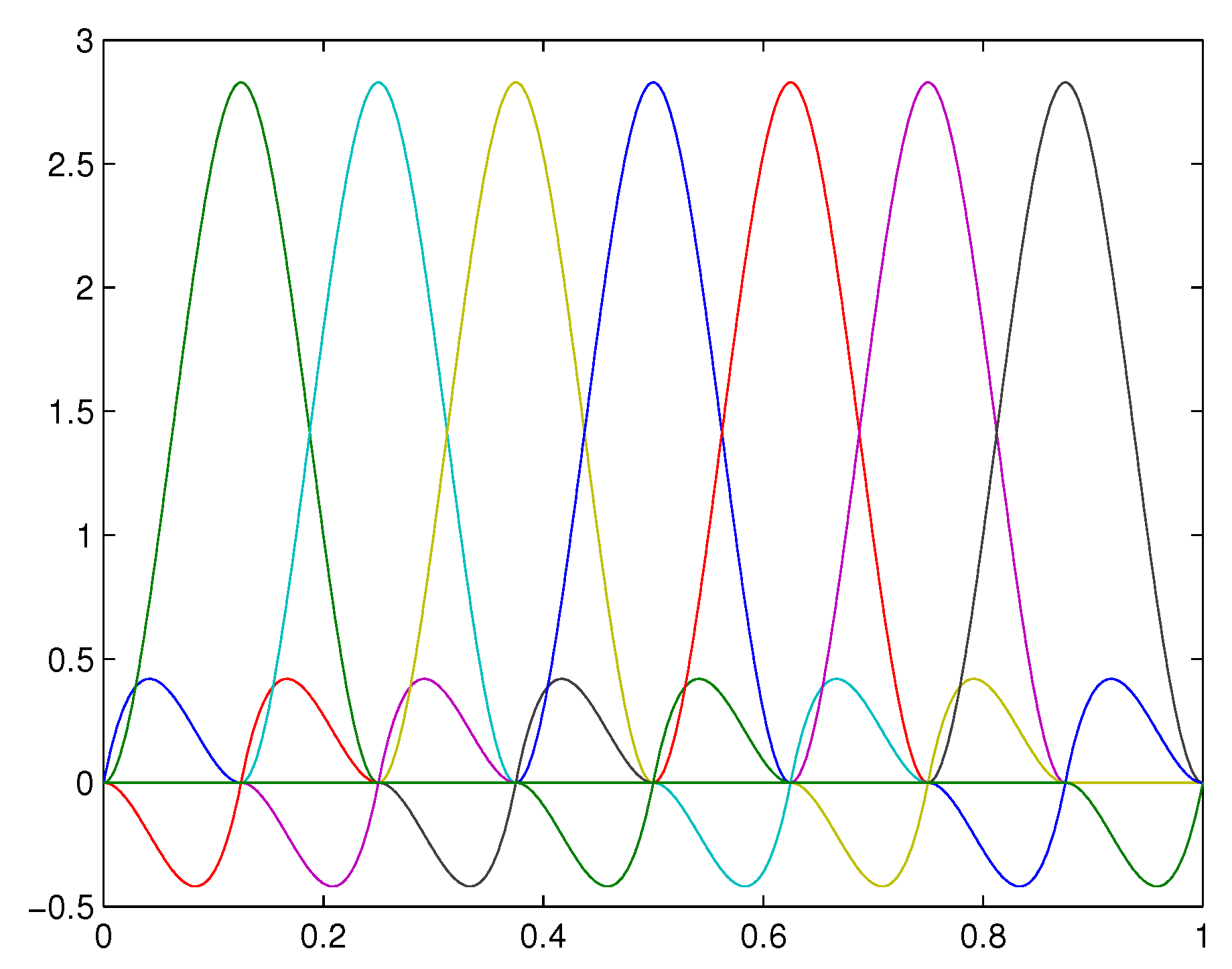
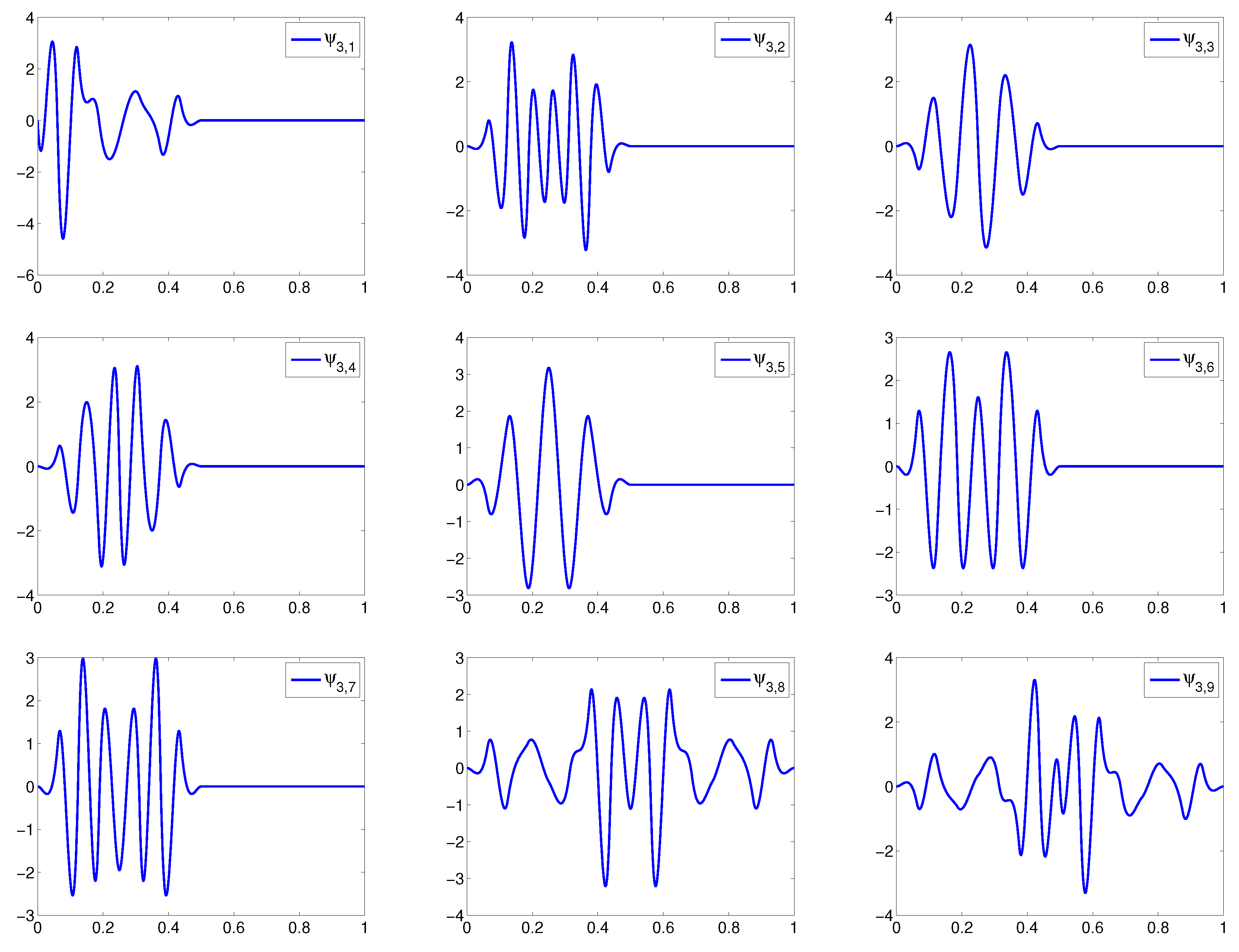
and after computing ${\psi }^b$ and ${\psi }^i$, $i=1,\dots ,8$, using these parameters, we normalize them with respect to the $L^2$-norm, i.e., we redefine ${\psi }^b:={\psi }^b/∥{\psi }^b∥$ and ${\psi }^i:={\psi }^i/∥{\psi }^i∥$. The wavelets ${\psi }_{3,1},\dots ,{\psi }_{3,9}$ that are dilations of ${\psi }^b,{\psi }^1,\dots ,{\psi }^8$ are displayed in Figure 2.

Theorem 4.

The sets ${\Psi }_j$ with the parameters given by (64) are uniform Riesz bases of $W_j$ for $j\ge 3$.

Proof of Theorem 5.

Since we constructed wavelets such that many of them are orthogonal, there is only a small number of nonzero entries in ${\mathbf{N}}_j$. Since wavelets are normalized with respect to the $L^2$-norm, we have:

$${\left({\mathbf{N}}_j\right)}_{k,k}=1.$$

(65)

Direct computation yields that:

$$\begin{array}{c}{\left({\mathbf{N}}_j\right)}_{k=1,l=2,\dots ,9}={\left({\mathbf{N}}_j\right)}_{k=2^j,l=2^j-1,\dots ,2^j-8}=\mathbf{z},\\ {\left({\mathbf{N}}_j\right)}_{k=2,\dots ,9,l=1}={\left({\mathbf{N}}_j\right)}_{k=2^j-1,\dots ,2^j-8,l=2^j}={\mathbf{z}}^T,\end{array}$$

(66)

where:

$$\mathbf{z}=\left(0.0022,-0.0927,-0.0166,-0.0339,-0.0075,0.0045,-0.2652,0.2439\right),$$

(67)

and for $i=1,\dots ,2^{j-2}-2$, we have:

$$\begin{array}{c}{\left({\mathbf{N}}_j\right)}_{k=8i,8i+1,l=8i+8,8i+9}=\mathbf{N}\\ {\left({\mathbf{N}}_j\right)}_{k=8i+8,8i+9,l=8i,8i+1}={\mathbf{N}}^T,\end{array}$$

(68)

where:

$$\mathbf{N}=\left(\begin{array}{cc}-0.2048& 0.1885\\ -0.1885& 0.1734\end{array}\right).$$

(69)

The numbers in (67) and (69) are rounded to four decimal digits. All other entries of ${\mathbf{N}}_j$ are zero. The structure of the Gram matrix ${\mathbf{N}}_j=〈{\Psi }_j,{\Psi }_j〉$ is displayed in Figure 3.

Using Gershgorin theorem, the smallest eigenvalue ${\lambda }_{min}\left({\mathbf{N}}_j\right)\ge 0.21$, and the largest eigenvalue ${\lambda }_{max}\left({\mathbf{N}}_j\right)\le 1.79$. Therefore, ${\Psi }_j$ are uniform Riesz bases of their spans. ☐

Theorem 5.

The set Ψ is a Riesz basis of $L^2\left(0,1\right)$, and when normalized with respect to the $H^1$-norm, it is a Riesz basis of $H_0^1\left(0,1\right)$.

Proof of Theorem 6.

Due to the Theorems 2, 3 and 4, the relation (29) holds both for $s=0$ and $s=1$. Hence, Ψ is a Riesz basis of $L^2\left(0,1\right)$ and:

$$\left\{2^{-3}{\varphi }_{3,k},k=1,\dots ,16\right\}\cup \left\{2^{-j}{\psi }_{j,k},j\ge 3,k=1,\dots ,2^{j+1}\right\}$$

(70)

is a Riesz basis of $H_0^1\left(0,1\right)$. To show that also:

$$\left\{\frac{{\varphi }_{3,k}}{{∥{\varphi }_{3,k}∥}_{H^1\left(0,1\right)}},k=1,\dots ,16\right\}\cup \left\{\frac{{\psi }_{j,k}}{{∥{\psi }_{j,k}∥}_{H^1\left(0,1\right)}},j\ge 3,k=1,\dots ,2^{j+1}\right\}$$

(71)

is a Riesz basis of $H_0^1\left(0,1\right)$, we follow the Proof of Theorem 2 in [40]. From (18) and (50) there exist nonzero constants $C_1$ and $C_2$, such that:

$$C_1{2}^j\le {∥{\psi }_{j,k}∥}_{H_0^1\left(\Omega \right)}\le C_2{2}^j,\mathrm{for}j\ge 3,k=1,\dots ,2^{j+1},$$

(72)

and:

$$C_1{2}^3\le {∥{\varphi }_{3,k}∥}_{H_0^1\left(\Omega \right)}\le C_2{2}^3,\mathrm{for}k=1,\dots ,16.$$

(73)

Let $\widehat{\mathbf{b}}=\left\{{\widehat{a}}_{3,k},k=1,\dots ,16\right\}\cup \left\{{\widehat{b}}_{j,k},j\ge 3,k=1,\dots ,2^{j+1}\right\}$ be such that:

$${∥\widehat{\mathbf{b}}∥}_2^2={\displaystyle \sum _{k=1}^{16}}{\widehat{a}}_{3,k}^2+{\displaystyle \sum _{j=3}^{\infty }}{\displaystyle \sum _{k=1}^{2^{j+1}}}{\widehat{b}}_{j,k}^2<\infty .$$

(74)

We define:

$$a_{3,k}=\frac{2^3{\widehat{a}}_{3,k}}{{∥{\varphi }_{3,k}∥}_{H_0^1\left(0,1\right)}},k=1,\dots ,16,b_{j,k}=\frac{2^j{\widehat{b}}_{j,k}}{{∥{\psi }_{j,k}∥}_{H_0^1\left(0,1\right)}},j\ge 3,k=1,\dots ,2^{j+1},$$

(75)

and $\mathbf{b}=\left\{a_{3,k},k=1,\dots ,16\right\}\cup \left\{b_{j,k},j\ge 3,k=1,\dots ,2^{j+1}\right\}$. Then:

$${∥\mathbf{b}∥}_2\le \frac{{∥\widehat{\mathbf{b}}∥}_2}{C_1}<\infty .$$

(76)

Since the set (70) is a Riesz basis of $H_0^1\left(0,1\right)$, there exist constants $C_3$ and $C_4$, such that:

$$C_3{∥\mathbf{b}∥}_2\le {∥{\displaystyle \sum _{k=1}^{16}}{a}_{3,k}{2}^{-3}{\varphi }_{3,k}+{\displaystyle \sum _{j=3}^{\infty }}{\displaystyle \sum _{k=1}^{2^{j+1}}}{b}_{j,k}{2}^{-j}{\psi }_{j,k}∥}_{H_0^1\left(0,1\right)}\le C_4{∥\mathbf{b}∥}_2.$$

(77)

Therefore:

$$\begin{array}{c}\frac{C_4}{C_1}{∥\widehat{\mathbf{b}}∥}_2\ge C_4{∥\mathbf{b}∥}_2\ge {∥{\displaystyle {\sum }_{k=1}^{16}}{a}_{3,k}{2}^{-3}{\varphi }_{3,k}+{\displaystyle {\sum }_{j=3}^{\infty }}{\displaystyle {\sum }_{k=1}^{2^{j+1}}}{b}_{j,k}{2}^{-j}{\psi }_{j,k}∥}_{H_0^1\left(0,1\right)}\\ ={∥{\displaystyle {\sum }_{k=1}^{16}}\frac{{\widehat{a}}_{3,k}}{{∥{\varphi }_{3,k}∥}_{H_0^1\left(0,1\right)}}{\varphi }_{3,k}+{\displaystyle {\sum }_{j=3}^{\infty }}{\displaystyle {\sum }_{k=1}^{2^{j+1}}}\frac{{\widehat{b}}_{j,k}}{{∥{\psi }_{j,k}∥}_{H_0^1\left(0,1\right)}}{\psi }_{j,k}∥}_{H_0^1\left(0,1\right)}\end{array}$$

(78)

and similarly:

$$\begin{array}{c}\hfill \frac{C_3}{C_2}{∥\widehat{\mathbf{b}}∥}_2\le {∥{\displaystyle \sum _{k=1}^{16}}\frac{{\widehat{a}}_{3,k}}{{∥{\varphi }_{3,k}∥}_{H_0^1\left(0,1\right)}}{\varphi }_{3,k}+{\displaystyle \sum _{j=3}^{\infty }}{\displaystyle \sum _{k=1}^{2^{j+1}}}\frac{{\widehat{b}}_{j,k}}{{∥{\psi }_{j,k}∥}_{H_0^1\left(0,1\right)}}{\psi }_{j,k}∥}_{H_0^1\left(0,1\right)}.\end{array}$$

(79)

☐

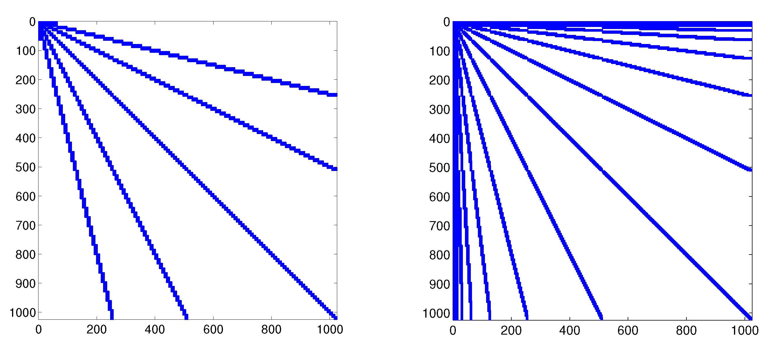
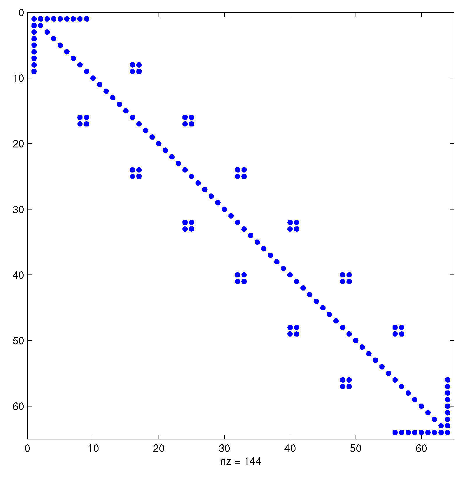
The condition number of the resulting wavelet basis with wavelets up to the level of 10 with respect to the $L^2$-norm is 17.2, and the condition number of this basis normalized with respect to the $H^1$-norm is 6.0. The sparsity pattern of the matrix arising from a discretization using a wavelet basis constructed in this paper and a wavelet basis from [25] for the one-dimensional Black–Scholes equation with quadratic volatilities from Example 1 is displayed in Figure 4.

5. Wavelets on the Hypercube

We present a well-known construction of a multivariate wavelet basis on the unit hypercube $\Omega ={\left(0,1\right)}^d$; for more details, see, e.g., [23]. It is based on tensorizing univariate wavelet bases and preserves the Riesz basis property, the locality of wavelets, vanishing moments and polynomial exactness. This approach is known as an anisotropic approach.

For notational simplicity, we denote ${\mathcal{J}}_j=\left\{1,\dots ,2^{j+1}\right\}$ for $j\ge 3$, and:

$${\psi }_{2,k}:={\varphi }_{3,k},k\in {\mathcal{J}}_2:={\mathcal{J}}_3,\mathcal{J}:=\left\{\left(j,k\right),j\ge 2,\in {\mathcal{J}}_j\right\}.$$

(80)

Then, we can write:

$$\Psi =\left\{{\psi }_{j,k},j\ge 2,k\in {\mathcal{J}}_j\right\}=\left\{{\psi }_{\lambda },\lambda \in \mathcal{J}\right\}.$$

(81)

We use $u\otimes v$ to denote the tensor product of functions u and v, i.e., $\left(u\otimes v\right)\left(x_1,x_2\right)=u\left(x_1\right)v\left(x_2\right)$. We define multivariate basis functions as:

$${\psi }_{\mathit{\lambda }}={\otimes }_{i=1}^d{\psi }_{{\lambda }_i},\mathit{\lambda }=\left({\lambda }_1,\dots ,{\lambda }_d\right)\in \mathbf{J},\mathbf{J}={\mathcal{J}}^d=\mathcal{J}\otimes \dots \otimes \mathcal{J}.$$

(82)

Since Ψ is a Riesz basis of $L^2\left(0,1\right)$ and Ψ normalized with respect to the $H^1$-norm is a Riesz basis of $H_0^1\left(0,1\right)$, the set:

$${\Psi }^{ani}:=\left\{{\psi }_{\mathit{\lambda }},\mathit{\lambda }\in \mathbf{J}\right\}$$

(83)

is a Riesz basis of $L^2\left(\Omega \right)$, and its normalization with respect to the $H^1$-norm is a Riesz basis of $H_0^1\left(\Omega \right)$. Using the same argument as in the Proof of Lemma 1, we conclude that for this basis, the discretization matrix is sparse for Equation (1) with piecewise polynomial coefficients on uniform meshes, such that $\mathrm{deg}{p}_{k,l}\le 6$, $\mathrm{deg}{q}_k\le 5$ and $\mathrm{deg}{a}_0\le 4$.

6. Numerical Examples

In this section, we solve the elliptic Equation (1) and the equation with the Black–Scholes operator from Example 1 by an adaptive wavelet method with the basis constructed in this paper. We briefly describe the algorithm. While the classical adaptive methods typically uses refining a mesh according to a posteriori local error estimates, the wavelet approach is different, and it comprises the following steps [13,17,18]:

• One starts with a variational formulation for a suitable wavelet basis, but instead of turning to a finite dimensional approximation, the continuous problem is transformed into an infinite-dimensional $l^2$-problem.
• Then, one proposes a convergent iteration for the $l^2$-problem.
• Finally, one derives an implementable version of this idealized iteration, where all infinite-dimensional quantities are replaced by finitely supported ones.

To the left-hand side of the Equation (1), we associate the following bilinear form:

$$a\left(v,w\right):={\int }_{\Omega }{\displaystyle \sum _{k,l=1}^d}{p}_{k,l}\frac{\partial v}{\partial x_k}\frac{\partial w}{\partial x_l}+{\displaystyle \sum _{k=1}^d}{q}_k\frac{\partial v}{\partial x_k}w+p_{0}vw\mathrm{d}x.$$

(84)

The weak formulation of (1) reads as follows: Find $u\in H_0^1\left(\Omega \right)$, such that:

$$a\left(u,v\right)=〈f,v〉\mathrm{for}\mathrm{all}v\in H_0^1\left(\Omega \right).$$

(85)

Instead of turning to a finite dimensional approximation, Equation (85) is reformulated as an equivalent bi-infinite matrix equation $\mathbf{A}\mathbf{u}=\mathbf{f}$, where:

$${\left(\mathbf{A}\right)}_{\lambda ,\mu }=a\left({\psi }_{\lambda },{\psi }_{\mu }\right),{\left(\mathbf{f}\right)}_{\lambda }=〈f,{\psi }_{\lambda }〉,$$

(86)

for ${\psi }_{\lambda },{\psi }_{\mu }\in \Psi$ and Ψ is a wavelet basis of $H_0^1\left(\Omega \right)$.

We use the standard Jacobi diagonal preconditioner $\mathbf{D}$ for preconditioning this equation, i.e., ${\mathbf{D}}_{\lambda ,\mu }={\mathbf{D}}_{\lambda ,\mu }{\delta }_{\lambda ,\mu }$. If the coefficients are constant, one can also use an efficient diagonal preconditioner from [41]. The algorithm for solving the $l^2$-problem is the following:

• Compute sparse representation ${\mathbf{f}}_j$ of the right-hand side $\mathbf{f}$, such that ${∥\mathbf{f}-{\mathbf{f}}_j∥}_2$ is smaller than a given tolerance ${ϵ}_j^1$. The computation of a sparse representation insists on thresholding the smallest coefficients and working only with the largest ones. We denote the routine as ${\mathbf{f}}_j:=\mathrm{RHS}[\mathbf{f},{ϵ}_j^1]$.
• Compute K steps of GMRESfor solving the system $\mathbf{A}\mathbf{v}={\mathbf{f}}_j$ with the initial vector ${\mathbf{v}}_j$. Each iteration of GMRES requires multiplication of the infinite-dimensional matrix with a finitely-supported vector. Since for the wavelet basis constructed in this paper, the matrix is sparse, it can be computed exactly. Otherwise, it is computed approximately with the given tolerance ${ϵ}_j^2$ by the method from [24]. We denote the routine $\mathbf{z}=\mathbf{GMRES}[\mathbf{A},{\mathbf{f}}_j,{\mathbf{v}}_j,K]$.
• Compute sparse representation ${\mathbf{v}}_{j+1}$ of $\mathbf{z}$ with the error smaller than ${ϵ}_j^2$. We denote the routine ${\mathbf{v}}_{j+1}:=\mathbf{COARSE}[\mathbf{z},{ϵ}_j^2]$. It insists on thresholding the coefficients.

We repeat Steps 1, 2 and 3 until the norm of the residual ${\mathbf{r}}_j={∥\mathbf{f}-\mathbf{A}{\mathbf{v}}_j∥}_2$ is not smaller than the required tolerance $\widetilde{ϵ}$. Since we work with the sparse representation of the right-hand side and the sparse representation of the vector representing the solution, the method is adaptive. It is known that the coefficients in the wavelet basis are small in regions where the function is smooth and large in regions where the function has some singularity. Therefore, by this method, the singularities are automatically detected.

We use the following algorithm that is a modified version of the original algorithm from [17,18]:

Algorithm 1 $u:=$SOLVE [ $\mathbf{A}$, $\mathbf{f}$, $\widetilde{ϵ}$ ]

1. Choose $k_0,k_1,k_2\in \left(0,1\right)$, $K\in \mathbb{N}$.

2. Set $j:=0$, ${\mathbf{v}}_0:=0$ and $ϵ:={∥\mathbf{f}∥}_2$.

3. While $ϵ>\widetilde{ϵ}$

$j:=j+1$,

$ϵ:=k_0ϵ$,

${ϵ}_j^1:=k_1ϵ$,

${ϵ}_j^2:=k_2ϵ$,

${\mathbf{f}}_j:=\mathbf{RHS}[\mathbf{f},{ϵ}_j^1]$,

$\mathbf{z}:=\mathbf{GMRES}[\mathbf{A},{\mathbf{f}}_j,{\mathbf{v}}_{j-1},K]$

${\mathbf{v}}_j:=\mathbf{COARSE}[\mathbf{z},{ϵ}_j^2]$,

Estimate ${\mathbf{r}}_j=\mathbf{f}-\mathbf{A}{\mathbf{v}}_j$ and set $ϵ:={∥{\mathbf{r}}_j∥}_2$.

end while,

4. $\mathbf{u}:={\mathbf{v}}_j$,

5. Compute approximate solution $\tilde{u}={\sum }_{u_{\lambda }\in \mathbf{u}}{u}_{\lambda }{\psi }_{\lambda }$.

For an appropriate choice of parameters $k_0,k_1,k_2$ and K and more details about the routines RHS and COARSE, we refer to [17,18,23].

Example 2.

We solve the equation:

$$-ϵu^{″}+x^2{u}^{\prime }+u=f\mathrm{on}\left(0,1\right),u\left(0\right)=u\left(1\right)=0,$$

(87)

where $ϵ=0.001$ and the right-hand side f is corresponding to the solution:

$$u\left(x\right)=x\left(1-e^{50x-50}\right)\mathrm{for}x\in \left[0,1\right].$$

(88)

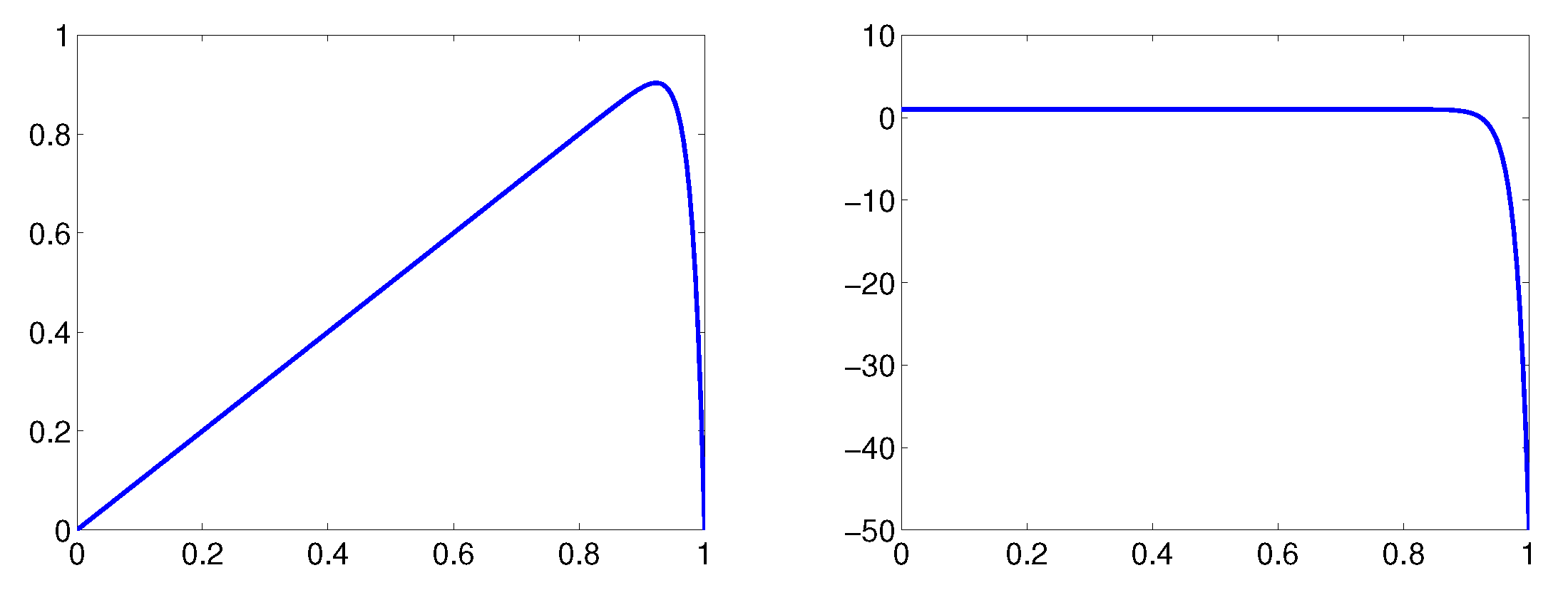
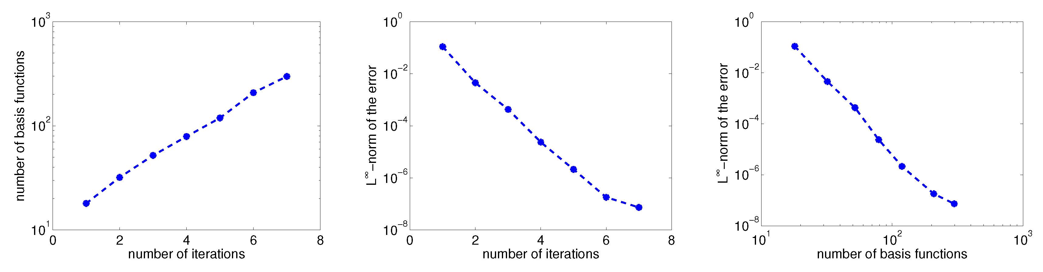
We solve this equation using the adaptive wavelet method described above with the wavelet basis constructed in this paper. The approximate solution and the derivative of the approximate solution that were computed using only 79 coefficients are displayed in Figure 5. The significant coefficients were located near Point 1, because the solution has a large derivative near this point.

The sparsity patterns of the matrices arising from discretization of Equation (87) using wavelets constructed in this paper and wavelets from [25] are the same as the sparsity patterns of matrices for Example 1 that are displayed in Figure 4. Convergence history is displayed in Figure 6. The number of iterations equals the parameter j from Algorithm 1; the number of basis functions determining the approximate solution in j-th iteration is the same as the number of nonzero entries of the vector ${\mathbf{v}}_j$; and the $L^{\infty }$-norm of the error is given by:

$${∥u-\tilde{u}∥}_{\infty }=\underset{x\in \left[0,1\right]}{\max }\left|u\left(x\right)-\tilde{u}\left(x\right)\right|.$$

(89)

Example 3.

We consider the equation:

$$\frac{\partial V}{\partial t}-{\displaystyle \sum _{k,l=1}^2}\frac{{\rho }_{k,l}}{2}{\sigma }_k{\sigma }_l{S}_k{S}_l\frac{{\partial }^{2}V}{\partial S_k\partial S_l}-r{\displaystyle \sum _{k=1}^2}{S}_k\frac{\partial V}{\partial S_k}+rV=f,$$

(90)

for $\left(S_1,S_2\right)\in \Omega :={\left(0,1\right)}^2$ and $t\in \left(0,1\right)$. We choose parameters of the Black–Scholes operator as ${\rho }_{1,1}={\rho }_{2,2}=1$, ${\rho }_{1,2}={\rho }_{2,1}=0.88$, ${\sigma }_1\left(x\right)=0.1x^2-0.1x+0.66$, ${\sigma }_2\left(x\right)=0.1x^2-0.1x+0.97$, $r=0.02$, and we set the right-hand side f, the initial and boundary conditions, such that the solution V is given by:

$$V\left(S_1,S_2,t\right)=e^{-rt}{S}_1{S}_2\left(1-e^{20S_1-20}\right)\left(1-e^{20S_2-20}\right)$$

(91)

for $\left(S_1,S_2,t\right)\in \Omega \times \left(0,1\right)$. We use the Crank–Nicolson scheme for the semi-discretization of the Equation (90) in time. Let $M\in \mathbb{N}$, $\tau =M^{-1}$, $t_l=l\tau$, $l=0,\dots ,M$, and denote $V_l\left(S_1,S_2\right)=V\left(S_1,S_2,t_l\right)$ and $f_l\left(S_1,S_2\right)=f\left(S_1,S_2,t_l\right)$. The Crank–Nicolson scheme has the form:

$$\frac{V_{l+1}-V_l}{\tau }-{\displaystyle \sum _{k,l=1}^2}\frac{{\rho }_{k,l}}{4}{\sigma }_k{\sigma }_l{S}_k{S}_l\frac{{\partial }^2\left(V_{l+1}+V_l\right)}{\partial S_k\partial S_l}-\frac{r}{2}{\displaystyle \sum _{k=1}^2}{S}_k\frac{\partial \left(V_{l+1}+V_l\right)}{\partial S_k}+\frac{r\left(V_{l+1}+V_l\right)}{2}=\frac{f_{l+1}+f_l}{2}.$$

(92)

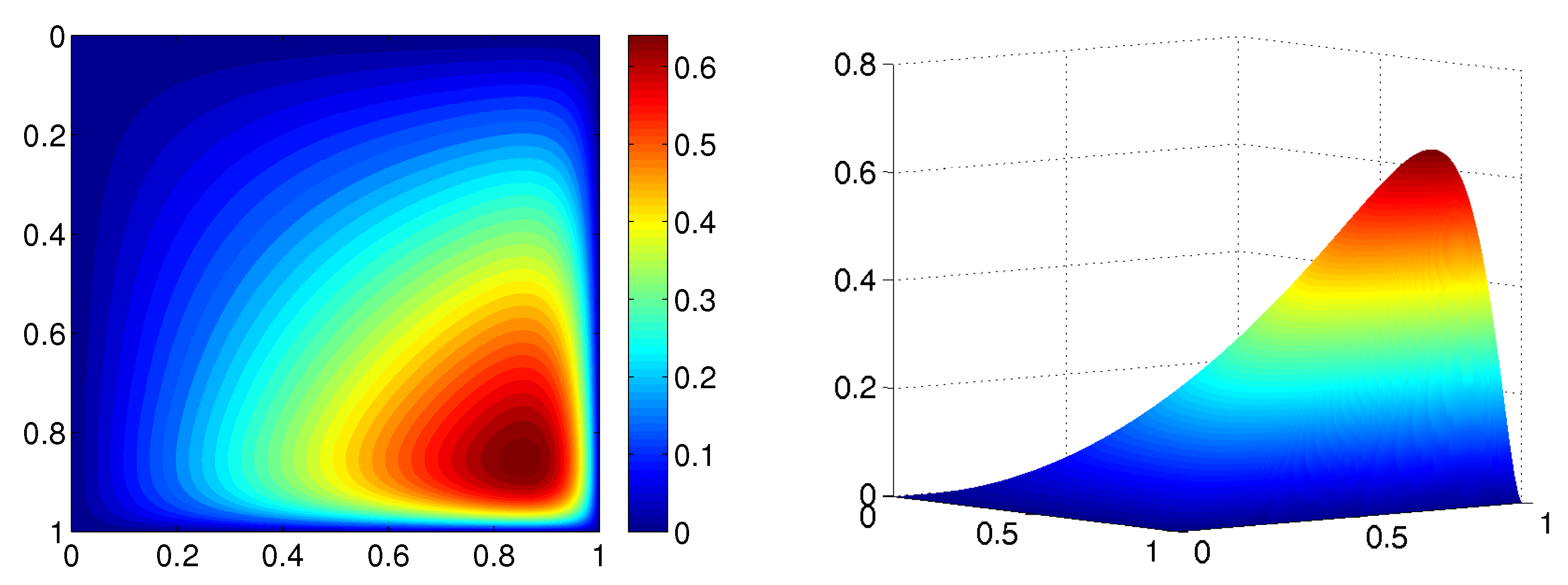
In this scheme, the function $V_l$ is known from the equation on the previous time level, and the function $V_{l+1}$ is an unknown solution. Thus, for the given time level $t_l$, Equation (92) is of the form (1), and we can use the adaptive wavelet method for solving it. The approximate solution $V_1$ for $\tau =1/365$ that was computed using 731 coefficients is displayed in Figure 7.

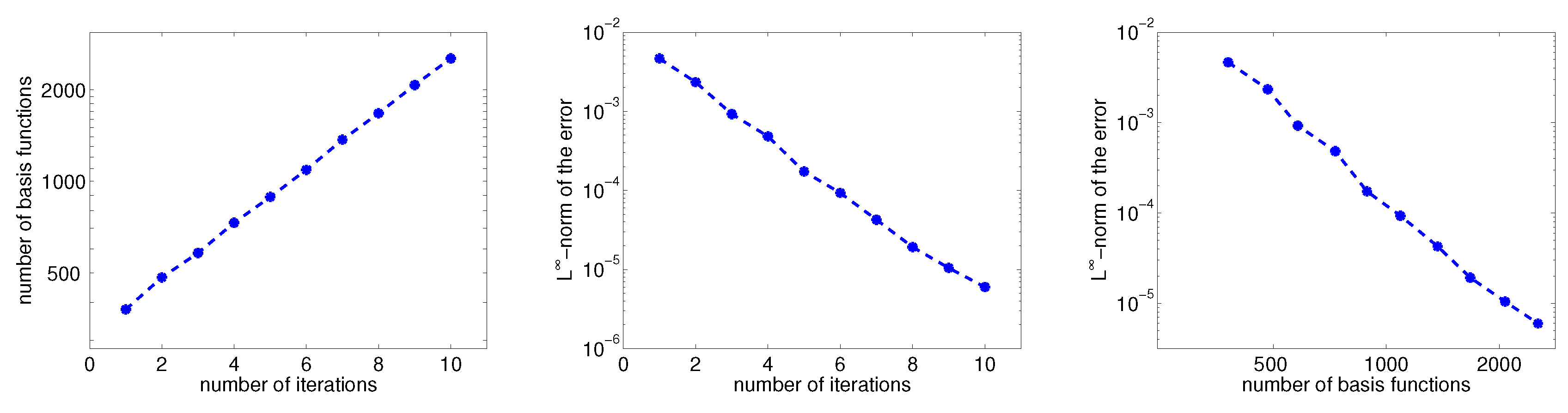
It can be seen that the gradient of the solution $V_1$ has the largest values near the point $\left[1,1\right]$. Therefore, the largest wavelet coefficients correspond to wavelets with supports in regions near this point, and wavelet coefficients are small for wavelets that are not located in these regions. Thus, many wavelet coefficients are omitted, and the representation of the solution is sparse. The convergence history is shown in Figure 8.

7. Conclusions

In this paper, we constructed a new cubic spline multi-wavelet basis on the unit interval and unit cube. The basis is adapted to homogeneous Dirichlet boundary conditions, and wavelets have eight vanishing moments. The main advantage of this basis is that the matrices arising from a discretization of the differential Equation (1) with piecewise polynomial coefficients on uniform meshes, such that $\mathrm{deg}{p}_{k,l}\le 6$, $\mathrm{deg}{q}_k\le 5$ and $\mathrm{deg}{a}_0\le 4$, are sparse and not only quasi-sparse. We proved that the constructed basis is indeed a wavelet basis, i.e., the Riesz basis property (5) is satisfied. We performed extensive numerical experiments and present the construction that leads to the wavelet basis that is well-conditioned with respect to the $L^2$-norm, as well as the $H^1$-norm.

References

Beylkin, G. Wavelets and fast numerical algorithms. In Different Perspectives on Wavelets 47; Daubechies, I., Ed.; Proceedings of Symposia in Applied Mathematics; American Mathematical Society: Providence, RI, USA, 1993; pp. 89–117. [Google Scholar]
Shann, W.C.; Xu, J.C. Galerkin-wavelet methods for two-point boundary value problems. Numer. Math.1992, 63, 123–142. [Google Scholar]
Hariharan, G.; Kannan, K. Haar wavelet method for solving some nonlinear parabolic equations. J. Math. Chem.2010, 48, 1044–1061. [Google Scholar] [CrossRef]
Lepik, Ü. Numerical solution of differential equations using Haar wavelets. Math. Comput. Simul.2005, 68, 127–143. [Google Scholar] [CrossRef]
Lepik, Ü. Numerical solution of evolution equations by the Haar wavelet method. Appl. Math. Comput.2007, 185, 695–704. [Google Scholar] [CrossRef]
Cattani, C. Haar wavelet spline. J. Interdiscip. Math.2001, 4, 35–47. [Google Scholar] [CrossRef]
Cattani, C.; Bochicchio, I. Wavelet analysis of chaotic systems. J. Interdiscip. Math.2006, 9, 445–458. [Google Scholar]
Ciancio, A.; Cattani, C. Analysis of Singularities by Short Haar Wavelet Transform. In Lecture Notes in Computer Science; Gervasi, O., Kumar, V., Tan, C.J.K., Taniar, D., Laganá, A., Mun, Y., Choo, H., Eds.; Springer: Berlin/Heidelberg, Germany, 2006; pp. 828–838. [Google Scholar]
Kumar, V.; Mehra, M. Cubic spline adaptive wavelet scheme to solve singularly perturbed reaction diffusion problems. Int. J. Wavelets Multiresolut. Inf. Process.2007, 15, 317–331. [Google Scholar] [CrossRef]
Jia, R.Q.; Zhao, W. Riesz bases of wavelets and applications to numerical solutions of elliptic equations. Math. Comput.2011, 80, 1525–1556. [Google Scholar] [CrossRef]
Negarestani, H.; Pourakbari, F.; Tavakoli, A. Adaptive multiple knot B-spline wavelets for solving Saint-Venant equations. Int. J. Wavelets Multiresolut. Inf. Process.2013, 11, 1–12. [Google Scholar]
Mehra, M. Wavelets and differential equations—A short review. In AIP Conference Proceedings 1146; Siddiqi, A.H., Gupta, A.K., Brokate, M., Eds.; American Institute of Physics: New York, NY, USA, 2009; pp. 241–252. [Google Scholar]
Dahmen, W. Multiscale and wavelet methods for operator equations. Lect. Notes Math.2003, 1825, 31–96. [Google Scholar]
Caflisch, R.E.; Gargano, F.; Sammartino, M.; Sciacca, V. Complex singularities and PDEs. Rivista Matematica Universita di Parma2015, 6, 69–133. [Google Scholar]
Gargano, F.; Sammartino, M.; Sciacca, V.; Cassel, K.V. Analysis of complex singularities in high-Reynolds-number Navier-Stokes solutions. J. Fluid Mech.2014, 747, 381–421. [Google Scholar] [CrossRef]
Weideman, J.A.C. Computing the dynamics of complex singularities of nonlinear PDEs. SIAM J. Appl. Dyn. Syst.2003, 2, 171–186. [Google Scholar] [CrossRef]
Urban, K. Wavelet Methods for Elliptic Partial Differential Equations; Oxford University Press: Oxford, UK, 2009. [Google Scholar]
Černá, D.; Finěk, V. Approximate multiplication in adaptive wavelet methods. Cent. Eur. J. Math.2013, 11, 972–983. [Google Scholar] [CrossRef]
Dijkema, T.J.; Stevenson, R. A sparse Laplacian in tensor product wavelet coordinates. Numer. Math.2010, 115, 433–449. [Google Scholar] [CrossRef]
Cvejnová, D.; Černá, D.; Finěk, V. Hermite cubic spline multi-wavelets on the cube. In AIP Conference Proceedings 1690; Pasheva, V., Popivanov, N., Venkov, G., Eds.; American Institute of Physics: New York, NY, USA, 2015; No. 030006. [Google Scholar]
Černá, D.; Finěk, V. On a sparse representation of an n-dimensional Laplacian in wavelet coordinates. Results Math.2016, 69, 225–243. [Google Scholar] [CrossRef]
Černá, D. Numerical solution of the Black–Scholes equation using cubic spline wavelets. In AIP Conference Proceedings 1789; Pasheva, V., Popivanov, N., Venkov, G., Eds.; American Institute of Physics: New York, NY, USA, 2016; No. 030001. [Google Scholar]
Cvejnová, D.; Šimůnková, M. Comparison of multidimensional wavelet bases. AIP Conf. Proc.2015, 1690, 030008. [Google Scholar]
Schneider, A. Biorthogonal cubic Hermite spline multi-wavelets on the interval with complementary boundary conditions. Results Math.2009, 53, 407–416. [Google Scholar] [CrossRef]
Dahmen, W.; Han, B.; Jia, R.Q.; Kunoth, A. Biorthogonal multi-wavelets on the interval: Cubic Hermite splines. Constr. Approx.2000, 16, 221–259. [Google Scholar] [CrossRef]
Jia, R.Q.; Liu, S.T. Wavelet bases of Hermite cubic splines on the interval. Adv. Comput. Math.2006, 25, 23–39. [Google Scholar] [CrossRef]
Shumilov, B.M. Multiwavelets of the third-degree Hermitian splines orthogonal to cubic polynomials. Math. Models Comput. Simul.2013, 5, 511–519. [Google Scholar] [CrossRef]
Shumilov, B.M. Cubic multi-wavelets orthogonal to polynomials and a splitting algorithm. Numer. Anal. Appl.2013, 6, 247–259. [Google Scholar] [CrossRef]
Xue, X.; Zhang, X.; Li, B.; Qiao, B.; Chen, X. Modified Hermitian cubic spline wavelet on interval finite element for wave propagation and load identification. Finite Elem. Anal. Des.2014, 91, 48–58. [Google Scholar] [CrossRef]
Černá, D.; Finěk, V. Wavelet bases of cubic splines on the hypercube satisfying homogeneous boundary conditions. Int. J. Wavelets Multiresolut. Inf. Process.2015, 13, 1550014. [Google Scholar] [CrossRef]
Zuhlsdorff, C. The pricing of derivatives on assets with quadratic volatility. Appl. Math. Financ.2001, 8, 235–262. [Google Scholar] [CrossRef]
Dahmen, W. Stability of multiscale transformations. J. Fourier Anal. Appl.1996, 4, 341–362. [Google Scholar]
Johnson, C.R. A Gershgorin-type lower bound for the smallest singular value. Linear Algebra Appl.1989, 112, 1–7. [Google Scholar] [CrossRef]
Černá, D.; Finěk, V. Quadratic spline wavelets with short support for fourth-order problems. Results Math.2014, 66, 525–540. [Google Scholar] [CrossRef]
Černá, D.; Finěk, V. A diagonal preconditioner for singularly pertubed problems. Bound. Value Probl.2017, 2017, 22. [Google Scholar] [CrossRef]
Figure 1.
Scaling functions on the level .
Figure 2.
Wavelets .
Figure 3.
The structure of the matrix .
Figure 4.
The sparsity pattern of the matrices arising from a discretization using a wavelet basis constructed in this paper (left) and a wavelet basis from [25] (right) for the Black–Scholes equation with quadratic volatilities.
Figure 5.
The approximate solution (left) and the derivative of the approximate solution (right) for Example 1.
Figure 6.
Convergence history for Example 1. The number of basis functions and the -norm of the error are in logarithmic scaling.
Figure 7.
Contour plot (left) and 3D plot (right) of the approximate solution for Example 2.
Figure 8.
Convergence history for Example 2. The number of basis functions and the -norm of the error are in logarithmic scaling.
Černá, D.; Finĕk, V.