
Multivariate Extended Gamma Distribution

Department of Statistics, Kuriakose Elias College, Mannanam, Kottayam, Kerala 686561, India
Axioms 2017, 6(2), 11; https://doi.org/10.3390/axioms6020011
Submission received: 7 June 2016
/
Revised: 7 April 2017
/
Accepted: 13 April 2017
/
Published: 24 April 2017
(This article belongs to the Special Issue Special Functions: Fractional Calculus and the Pathway for Entropy Dedicated to Professor Dr. A.M. Mathai on the occasion of his 80th Birthday)
Abstract
:In this paper, I consider multivariate analogues of the extended gamma density, which will provide multivariate extensions to Tsallis statistics and superstatistics. By making use of the pathway parameter , multivariate generalized gamma density can be obtained from the model considered here. Some of its special cases and limiting cases are also mentioned. Conditional density, best predictor function, regression theory, etc., connected with this model are also introduced.
1. Introduction
Consider the generalized gamma density of the form
where is the normalizing constant. Note that this is the generalization of some standard statistical densities such as gamma, Weibull, exponential, Maxwell-Boltzmann, Rayleigh and many more. We will extend the generalized gamma density by using pathway model of [1] and we get the extended function as
where is the normalizing constant.
Note that is a generalized type-2 beta model. Also so that it can be considered to be an extended form of . For various values of the pathway parameter a path is created so that one can see the movement of the function denoted by above towards a generalized gamma density. From the Figure 1 we can see that, as moves away from 1 the function moves away from the origin and it becomes thicker tailed and less peaked. From the path created by we note that we obtain densities with thicker or thinner tail compared to generalized gamma density. Observe that for , writing in Equation (2) produce generalized type-1 beta form, which is given by
where is the normalizing constant (see [2]).
2. Multivariate Extended Gamma
Various multivarite generalizatons of pathway model are discussed in the papers of Mathai [10,11]. Here we consider the multivariate case of the extended gamma density of the form (2). For let
where is the normalizing constant, which will be given later. This multivariate analogue can also produce multivariate extensions to Tsallis statistics [5,12] and superstatistics [3]. Here the variables are not independently distributed, but when we have a result that will become independently distributed generalized gamma variables. That is,
where
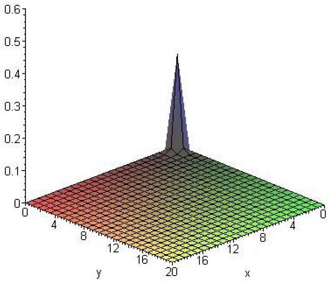
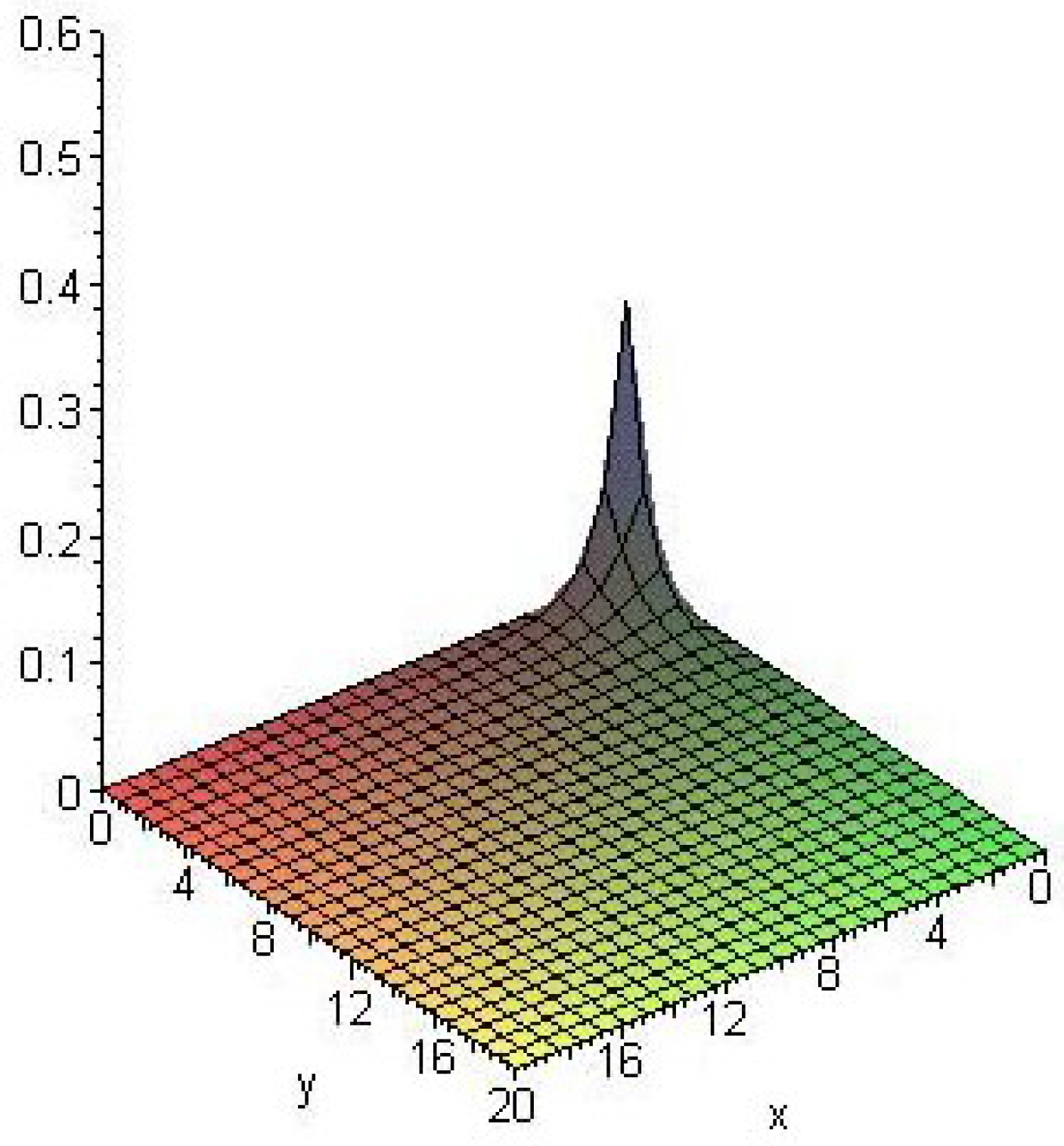
The following are the graphs of 2-variate extended gamma with and for various values of the pathway parameter From the Figure 2, Figure 3 and Figure 4, we can see the effect of the pathway parameter in the model.
Special Cases and Limiting Cases
- When → 1, (3) will become independently distributed generalized gamma variables. This includes multivariate analogue of gamma, exponential, chisquare, Weibull, Maxwell- Boltzmann, Rayleigh, and related models.
- If , (3) is identical with type-2 beta density.
A sample of the surface for is given in the Figure 5.
3. Marginal Density
We can find the marginal density of , by integrating out . First let us integrate out then the joint density of denoted by is given by
where By putting and integrating we get
In a similar way we can integrate out . Then the marginal density of is denoted by and is given by
where
If we take any subset of the marginal densities belong to the same family. In the limiting case they will also become independently distributed generalized gamma variables.
Normalizing Constant
4. Joint Product Moment and Structural Representations
Let have a multivariate extended gamma density (23). By observing the normalizing constant in (9), we can easily obtained the joint product moment for some arbitrary ,
Property 1.
The joint product moment of the multivariate extended gamma density can be written as
where ’ s are generalized gamma random variables having density function
where is the normalizing constant.
Property 2.
Letting in (10), we get
(13) is the moment of a random variable with density function of the the form (8),
where is the normalizing constant. Then
Making the substitution , then it will be in the form of a type-2 beta density and we can easily obtained the moment as in (13).
Property 3.
Letting in (10), we get
which is the joint product moment of a bivariate extended gamma density is denoted by and is given by
where is the normalizing constant. (17) is obtained by integrating out from (3). By putting in (10), we get the joint product moment of trivariate extended gamma density and so on.
Theorem 1.
When has density in (3), then
Corollary 1.
4.1. Variance-Covariance Matrix
Let X be a vector. Variance-covariance matrix is obtained by taking . Then the elements will be of the form
where
and
4.2. Normalizing Constant
Integrate out from (8) and equate with 1, we will get the normalizing constant as
5. Regression Type Models and Limiting Approaches
The conditional density of given is denoted by and is given by
where is the joint density of . When we take the limit as in Equation (24), we can see that the conditional density will be in the form of a generalized gamma density and is given by
Theorem 2.
Best Predictor
The conditional expectation, , is the best predictor, best in the sense of minimizing the expected squared error. Variables which are preassigned are usually called independent variables and the others are called dependent variables. In this context, is the dependent variable or being predicted and are the preassigned variables or independent variables. This ‘best’ predictor is defined as the regression function of on .
We can integrate the above integral as in the case of Equation (6). Then after simplification we will get the best predictor of at preassigned values of which is given by
We can take the limit in (27). For taking limit, let us apply Stirling’s approximations for gamma functions, see for example [15]
to the gamma’s in (27). Then we will get
which is the moment of a generalized gamma density as given in (25).
6. Multivariate Extended Gamma When
Consider the case when the pathway parameter is less than 1, then the pathway model has the form
and K is the normalizing constant. is the generalized type-1 beta model. Let us consider a multivariate case of the above model as
where is the normalizing constant and it can be obtained by solving
Integration over yields the following,
where and Letting then the above integral becomes a type-1 Dirichlet integral and the normalizing constant can be obtained as
When , (31) will become the density of independently distributed generalized gamma variables. By observing the normalizing constant in (34), we can easily obtaine the joint product moment for some arbitrary ,
Letting in (35), we get
(13) is the moment of a random variable with density function,
where is the normalizing constant.
If we proceed in the similar way as in Section 4.1, here we can deduce the variance-covariance matrix of multivariate extended gamma for .
7. Conclusions
Multivariate counterparts of the extended generalized gamma density is considered and some properties are discussed. Here we considered the variables as not independently distributed, but when the pathway parameter we can see that will become independently distributed generalized gamma variables. Joint product moment of the multivariate extended gamma is obtained and some of its properties are discussed. We can see that the limiting case of the conditional density of this multivariate extended gamma is a generalized gamma density. A graphical representation of the pathway is given in Figure 1, Figure 2, Figure 3 and Figure 4.
Acknowledgments
The author acknowledges gratefully the encouragements given by Professor A. M. Mathai, Department of Mathematics and Statistics, McGill University, Montreal, QC, Canada in this work.
Conflicts of Interest
The author declares no conflict of interest.
References
- Mathai, A.M. A Pathway to matrix-variate gamma and normal densities. Linear Algebra Appl. 2005, 396, 317–328. [Google Scholar] [CrossRef]
- Joseph, D.P. Gamma distribution and extensions by using pathway idea. Stat. Pap. Ger. 2011, 52, 309–325. [Google Scholar] [CrossRef]
- Beck, C.; Cohen, E.G.D. Superstatistics. Physica A 2003, 322, 267–275. [Google Scholar] [CrossRef]
- Beck, C. Stretched exponentials from superstatistics. Physica A 2006, 365, 96–101. [Google Scholar] [CrossRef]
- Tsallis, C. Possible generalizations of Boltzmann-Gibbs statistics. J. Stat. Phys. 1988, 52, 479–487. [Google Scholar] [CrossRef]
- Mathai, A.M.; Haubold, H.J. Pathway model, superstatistics Tsallis statistics and a generalized measure of entropy. Physica A 2007, 375, 110–122. [Google Scholar] [CrossRef]
- Kotz, S.; Balakrishman, N.; Johnson, N.L. Continuous Multivariate Distributions; John Wiley & Sons, Inc.: New York, NY, USA, 2000. [Google Scholar]
- Mathai, A.M.; Moschopoulos, P.G. On a form of multivariate gamma distribution. Ann. Inst. Stat. Math. 1992, 44, 106. [Google Scholar]
- Furman, E. On a multivariate gamma distribution. Stat. Probab. Lett. 2008, 78, 2353–2360. [Google Scholar] [CrossRef]
- Mathai, A.M.; Provost, S.B. On q-logistic and related models. IEEE Trans. Reliab. 2006, 55, 237–244. [Google Scholar] [CrossRef]
- Haubold, H.J.; Mathai, A.M.; Thomas, S. An entropic pathway to multivariate Gaussian density. arXiv, 2007; arXiv:0709.3820v. [Google Scholar]
- Tsallis, C. Nonextensive Statistical Mechanics and Thermodynamics. Braz. J. Phys. 1999, 29, 1–35. [Google Scholar]
- Thomas, S.; Jacob, J. A generalized Dirichlet model. Stat. Probab. Lett. 2006, 76, 1761–1767. [Google Scholar] [CrossRef]
- Thomas, S.; Thannippara, A.; Mathai, A.M. On a matrix-variate generalized type-2 Dirichlet density. Adv. Appl. Stat. 2008, 8, 37–56. [Google Scholar]
- Mathai, A.M. A Handbook of Generalized Special Functions for Statistical and Physical Sciences; Oxford University Press: Oxford, UK, 1993; pp. 58–116. [Google Scholar]
Figure 1.
The graph of , for and for various values of .
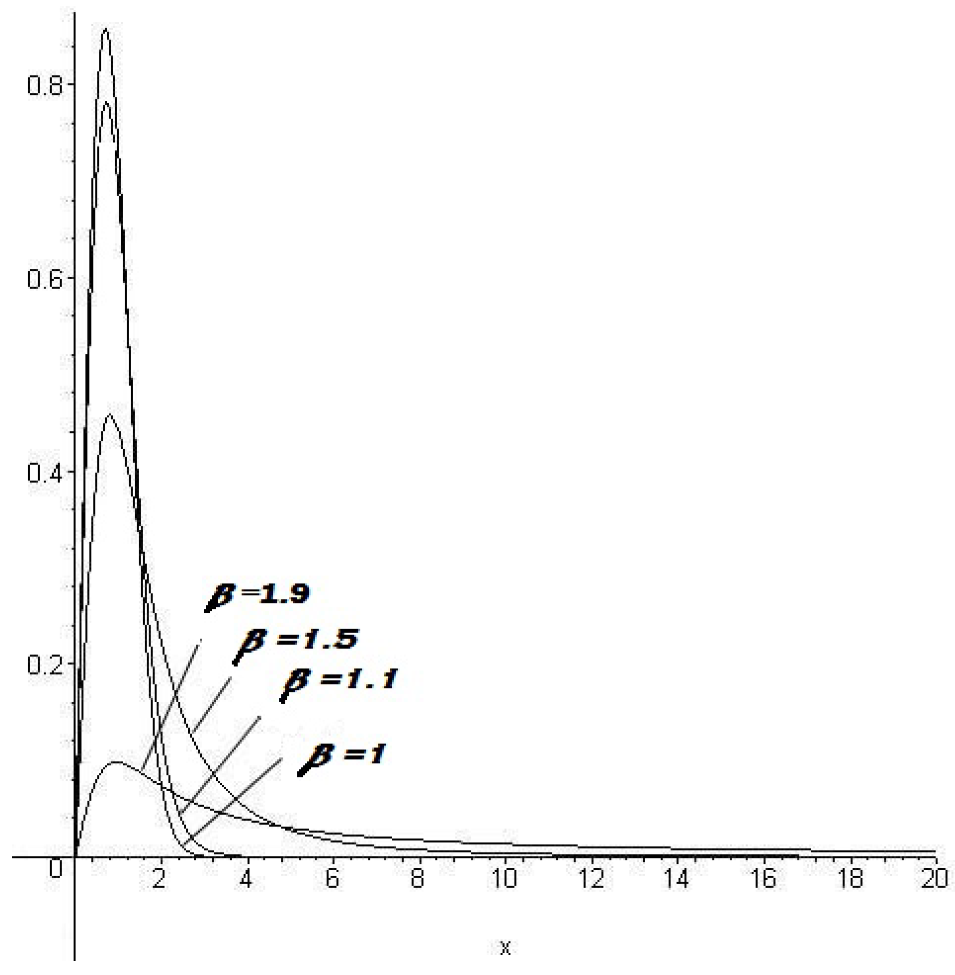
Figure 2.
.
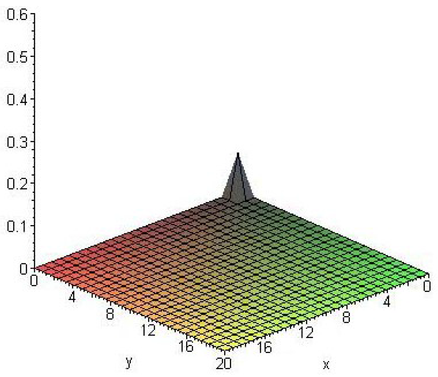
Figure 3.
.

Figure 4.
.

Figure 5.
The graph of bivariate type-2 Dirichlet with
© 2017 by the author. Licensee MDPI, Basel, Switzerland. This article is an open access article distributed under the terms and conditions of the Creative Commons Attribution (CC BY) license (http://creativecommons.org/licenses/by/4.0/).
Share and Cite
MDPI and ACS Style
Joseph, D.P. Multivariate Extended Gamma Distribution. Axioms 2017, 6, 11. https://doi.org/10.3390/axioms6020011
AMA Style
Joseph DP. Multivariate Extended Gamma Distribution. Axioms. 2017; 6(2):11. https://doi.org/10.3390/axioms6020011
Chicago/Turabian StyleJoseph, Dhannya P. 2017. "Multivariate Extended Gamma Distribution" Axioms 6, no. 2: 11. https://doi.org/10.3390/axioms6020011
Note that from the first issue of 2016, this journal uses article numbers instead of page numbers. See further details here.