A Fuzzy Trade-Off Ranking Method for Multi-Criteria Decision-Making


1
School of Mechanical, Aerospace and Civil Engineering, The University of Manchester, Sackville Street, Manchester M13 9PL, UK
2
Moscow Institute of Physics and Technology, 141700 Dolgoprudny, Russia
*
Author to whom correspondence should be addressed.
Axioms 2018, 7(1), 1; https://doi.org/10.3390/axioms7010001
Submission received: 9 November 2017
/
Revised: 16 December 2017
/
Accepted: 18 December 2017
/
Published: 26 December 2017
(This article belongs to the Special Issue Multi-Criteria Decisions)
Abstract
:The aim of this paper is to present a trade-off ranking method in a fuzzy multi-criteria decision-making environment. The triangular fuzzy numbers are used to represent the imprecise numerical quantities in the criteria values of each alternative and the weight of each criterion. A fuzzy trade-off ranking method is developed to rank alternatives in the fuzzy multi-criteria decision-making problem with conflicting criteria. The trade-off ranking method tackles this type of multi-criteria problems by giving the least compromise solution as the best option. The proposed method for the fuzzy decision-making problems is compared against two other fuzzy decision-making approaches, fuzzy Technique for Order Preference by Similarity to the Ideal Solution (TOPSIS) and fuzzy VlseKriterijuska Optimizacija I Komoromisno Resenje (VIKOR), used for ranking alternatives.
1. Introduction
In a conflicting multi-criteria problem, there is no unique solution that could optimize all the criteria simultaneously. The conflicting multi-criteria problem gives a set of Pareto solutions. Each Pareto solution is defined as a trade-off solution between the conflicting criteria, where it is not possible to achieve the best score of a criterion without downgrading the score of some other criteria.
The multi-criteria decision-making (MCDM) analysis contains a number of decision-making steps including weighting of criteria and ranking of alternatives. The weighting of criteria can reflect the individual preferences of the Decision-Maker. The weighted sum of the objectives leads to an aggregate function to be optimized. Eckenrode [1] implemented this approach to optimize an air-defence system. The selection of the alternatives was based on the individual preferences of 24 experts who considered six criteria.
The Analytic Hierarchy Process (AHP) proposed by Saaty [2] also involves human judgement in evaluations. According to AHP, the MCDM problem is split into a hierarchy with the goal, decision criteria and alternatives. Then, it uses the expert judgement to be converted into a numerical evaluation. The AHP is widely used in the decision-making process (e.g., [3,4,5,6,7]). Zaidan et al. [8] integrated the AHP method with other MCDM techniques to select the right software for open-source electronic medical record. The Analytic Network Process (ANP) also proposed by Saaty [9] represents some modification of the AHP. The ANP interprets the AHP hierarchy as a network. In contrast to the AHP, the decision criteria in the AHP are supposed to be independent from each another. This technique has been used in a number of publications (e.g., [10,11,12,13]).
The Multi-Attribute Utility Theory (MAUT) by Keeney and Raiffa [14] represents a classical approach in MCDM analysis. This is a structured methodology based on the utility axioms introduced by von Neumann and Morgenstern. In the algorithm, a utility value is assigned to each action whilst quantifying all individual preferences. Some examples of the use of MAUT in the decision-making can be found in [15]. In turn, the Elimination and Choice Expressing Reality (ELECTRE) by Roy is an outranking approach that is used to discard unacceptable alternatives. This approach was modified in PROMETHEE (Preference Ranking Organization Method for Enrichment Evaluations) by Brans and Vincke [16]. PROMETHEE exists in three versions: the PROMETHEE I (partial ranking), the PROMETHEE II (complete ranking) and the PROMETHEE-GAIA (geometrical analysis for interactive aid). Several authors applied the outranking techniques in MCDM problems (e.g., [17,18,19]).
The genetic algorithm (GA) has also been used for MCDM problems (e.g., [20,21,22,23,24]). It is widely used thanks to its universal nature. A problem with GA is that it generates a large number of solutions that are mostly redundant. Wang and Yang [25] used the particle swarm optimization (PSO) to determine a ranking for MCDM problems. Particle swarm is capable of improving the search ability of GA thanks to its better convergence to the Pareto frontier. However, as noted in [25], PSO requires significant computational time.
There is a number of techniques related to the ranking of available alternatives that are presented by the Pareto solutions. In all these techniques, the ranking is based on a metric introduced in the criteria space. The Technique for Order Preference by Similarity to the Ideal Solution (TOPSIS) was first proposed by Hwang and Yoon [26]. The original TOPSIS method presumed priori weights for criteria to be specified by the Decision-Maker. The TOPSIS approach is based on an individual evaluation score that depends on the distances from the alternative to the ideal and anti-ideal solutions. This type of evaluation is obviously the best for the non-conflicting multi-criteria problems, where the alternative that is the closest to the ideal solution is also the farthest from the anti-ideal solution. However, in a conflicting multi-criteria problem, such an assumption cannot always be realized. This drawback in TOPSIS is addressed in a few papers [27,28,29]. It was Kao [29] who practically suggested to measure the distance in norm instead of -norm implemented in the conventional TOPSIS method to overcome the inconsistency problem. TOPSIS has been widely used in MCDM due to its simplicity (e.g., [30,31,32,33]). The VlseKriterijuska Optimizacija I Komoromisno Resenje (VIKOR) algorithm proposed by Opricovic [27] is based on the compromise programming with weights to be prescribed to the performances by the Decision-Maker. Such weights are subjective and depend on how adequately such quantitative characteristics reflect the individual preferences of the Decision-Maker.
The real-life design is usually related to the inevitable uncertainties in the input data, parameters, etc. The uncertainty in the MCDM problem includes the imprecision of criteria values, vagueness in the importance of criteria (weights) and dealing with qualitative, linguistic or incomplete information.
The concept of fuzziness, first introduced by Zadeh [34], is proved to be an efficient tool to include the uncertainties in the MCDM problems. Numerous fuzzy MCDM methods have been developed, including [35,36,37,38,39,40,41,42]. They utilize the fuzzy numbers in the formulation of their fuzzy MCDM methods. There are two ways used in solving the fuzzy MCDM problems [43]. One way to solve the fuzzy MCDM problem is based on utilizing the fuzzy MCDM method [44,45]. Another way is reduced to the defuzzification of the fuzzy MCDM problem and solving it by a conventional MCDM method [46]. The defuzzification process converts the fuzzy numbers into crisp values. In both ways, the defuzzification process is essential, since the MCDM solution must provide a crisp result. Many defuzzification methods can be used including the center of sum and the center of gravity [47,48]. The fuzzy methodology was extended to the TOPSIS method [30,49,50,51] and VIKOR algorithm [52,53]. Several researchers used the fuzzy TOPSIS method for different applications including the selection problem [37,54,55,56] and the performance evaluation [40,57,58,59,60]. Wang et al. [28] proposed merging the fuzzy TOPSIS and the fuzzy AHP to surpass the problem. A few authors also explored the VIKOR algorithm to solve the fuzzy MCDM problem [61,62]. The trade-off ranking method [63] suggested by Jaini and Utyuzhnikov selects the least compromise solution as the best option. In contrast to the TOPSIS and VIKOR methodologies, the trade-off ranking method is based on the overall evaluation score of an alternative with respect to all other alternatives by taking into account the position of each Pareto solution in the criteria space. This strategy is nonlocal and essentially different from the VIKOR and TOPSIS methodologies.
The current paper is focused on the ranking of alternatives in the MCDM problems with conflicting criteria. The trade-off ranking method has been modified for a conflicting fuzzy environment. The approach is compared against the fuzzy TOPSIS and VIKOR methodologies. The paper is organized as follows. The next section briefly describes the fuzzy MCDM problem and its ranking application, the arithmetics of fuzzy numbers used throughout the paper, as well as the fuzzy VIKOR and TOPSIS methods. The background of the proposed fuzzy trade-off ranking method and its algorithms are discussed in Section 3. The approach is realized in both the fuzzy and defuzzification ways. In Section 4, a numerical example is presented to illustrate the application of the fuzzy trade-off ranking. The comparisons of the results are also given there. Lastly, the conclusions of the paper are discussed in Section 5.
2. Ranking Alternatives in Fuzzy Multi-Criteria Decision-Making
2.1. Fuzzy Multi-Criteria Decision-Making
A conventional MCDM problem can be expressed in a matrix form as
where the performance of criterion j in alternative i is represented by and the weight of each criterion is denoted by , for . Here, n is the number of criteria, and q is the number of alternatives.
| Criterion | ||||||
| Alternative | … | , | ||||
| … | ||||||
| … | ||||||
| … | ||||||
| ⋮ | ⋮ | ⋮ | ⋮ | ⋮ | ⋮ | |
| … | ||||||
Traditionally, the MCDM solutions assume all and values are crisp numbers. In reality, the values can be crisp, fuzzy or linguistic. For example, two candidates are considered for an engineer position. The criteria considered are creativity (), communication skill () and years of experience (). The rating for the first two criteria, and , are represented by linguistic terms such as “very good”, “average”, “poor”, and so on. The rating for criteria can be some integer numbers. Furthermore, for group decision-making that has K number of Decision-Makers (DMs), the preferences towards each criterion may be different for every DMs. In turn, each DM has his/her own uncertainty on the importance of each criterion. Thus, this MCDM problem contains the mixture of fuzzy, linguistic and crisp data set.
To tackle such a problem, the weights of the criteria, , and the performance of the alternative, , for the fuzzy MCDM problems are considered as linguistic variables, expressed in positive triangular fuzzy numbers, shown in Table 1 and Table 2 [30]. In turn, the membership function of linguistic variables in the alternative performance is presented in Figure 1.
Figure 1 shows the membership functions for the data stated in Table 1. As can be seen from Figure 1, the intervals to represent the linguistic variables are chosen in order to have a uniform representation from 0 to 10 in the triangular fuzzy numbers. The intervals are not unique and can have other representations [28,30,64,65,66].
Thus, a fuzzy MCDM problem can be expressed in a matrix form as
where the performance of criterion j in alternative i is now evaluated by the triangular fuzzy number and the weight of each criterion is represented by the triangular fuzzy number for . Again, n is the number of criteria, and q is the number of alternatives.
| Criterion | ||||||
| Alternative | … | , | ||||
| … | ||||||
| … | ||||||
| … | ||||||
| ⋮ | ⋮ | ⋮ | ⋮ | ⋮ | ⋮ | |
| … | ||||||
For group decision-making, consider a decision group that has a K number of DMs. Each DM is required to rate the performance of the alternatives and the weights of the criteria using the linguistic variables as in Table 1 and Table 2. The final values for the alternative performance with respect to each criterion and the weight of each criterion are considered as the average values from the rating scores, given by the formula:
Here, and are the fuzzy performances of the alternatives and the fuzzy weight of each criterion, evaluated by the K-th decision maker [30]. The operator ⊕, an addition of fuzzy numbers, is described further in the next section.
2.2. Arithmetic Operations on Triangular Fuzzy Numbers
In this section, several basic definitions and notations of fuzzy sets are briefly introduced. These definitions and notations are used throughout the paper for each fuzzy MCDM method.
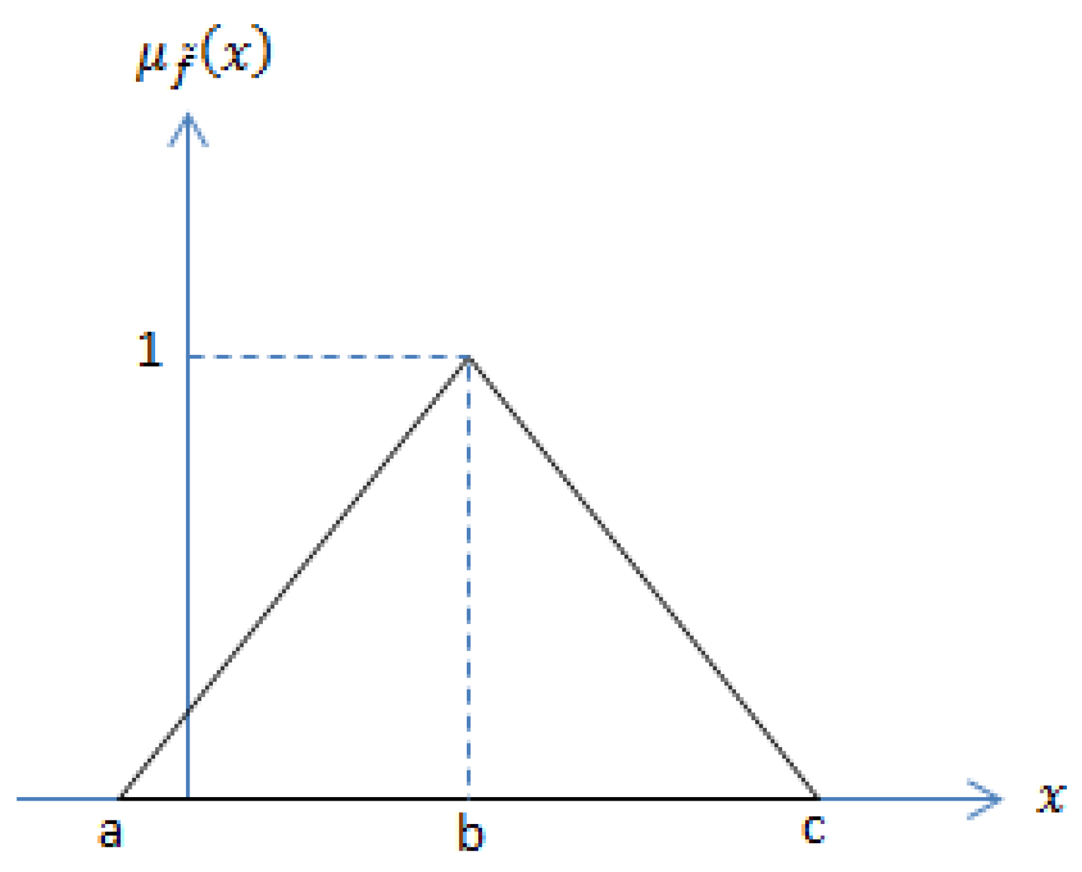
Figure 2 shows a triangular fuzzy number , where are real numbers. The interval reflects the fuzziness of the evaluation data b, where a closer interval means a lower degree of fuzziness. The membership function is defined as:
Given a real number r, some arithmetic operations on the fuzzy numbers are defined as follows:
The distance between two triangular fuzzy numbers, Equation (11), is also known as a vertex method [30]. In turn, the defuzzification, Equation (12), is known as the second weighted average formula [53]. As mentioned in Section 1, the defuzzification process turns the triangular fuzzy numbers into a crisp value. Such a process is the simplest way of tackling the fuzzy MCDM problem.
2.3. The Fuzzy TOPSIS Method
TOPSIS is based on the concept of having an alternative with the closest to the ideal solution and the farthest from the anti-ideal solution as the best option. The ideal and the anti-ideal solutions are considered as the artificial solutions.
The first step in the TOPSIS method is to normalize the decision matrix. To avoid the complicated normalization formula used in the classical TOPSIS, the linear normalization is used in the fuzzy TOPSIS [30]. Therefore, the normalized fuzzy decision matrix is given by equation:
where
and
Next, the weighted normalized fuzzy decision matrix is obtained by multiplying the weights with as:
Equation (6) is used for the multiplication of two fuzzy numbers. The Fuzzy Positive Ideal Solution (FPIS), and the Fuzzy Negative Ideal Solution (FNIS), are then defined as follows:
where and [30].
The distance for each weighted alternative to the FPIS and FNIS is computed using formulas:
where is the distance between two fuzzy numbers (11).
Finally, the closeness coefficient is calculated, in order to determine the ranking order of all alternatives, as follows:
The alternative with the highest closeness coefficient represents the best solution.
2.4. The Fuzzy VIKOR Method
Next, consider the basic formulation of the fuzzy VIKOR method. Assume the alternatives and the weights are evaluated by the triangular fuzzy numbers and respectively, for . The ranking algorithm for fuzzy VIKOR involves the following steps [53]:
- Determination of the ideal and the anti-ideal for , where
- (a)
- and , if the j-th criteria represents the benefit,
- (b)
- and , if the j-th criteria represents the cost.
The MAX and MIN are fuzzy operators as in Formulae (9) and (10), respectively. - Compute and , by the equationswith
- (a)
- , if the j-th criteria represents the benefit,
- (b)
- , if the j-th criteria represents the cost,
where is a normalized fuzzy difference, is a fuzzy weighted sum as in Equation (3) and is a fuzzy operator MAX (9). - “Core” ranking.Rank the alternatives by sorting the values of , . A lower value implies a higher ranking. The obtained ranking is denoted by .
- Fuzzy ranking.The i-th ranking position in is confirmed if , where and is the fuzzy numbers for alternative at the k-th position in . Confirmed ordering represents fuzzy ranking .
- Defuzzification of to convert the fuzzy numbers into crisp value using Equation (12).
- Defuzzification ranking.Rank the alternatives by sorting the crisp values of and Q in Step 6. A lower value implies a higher ranking. The results of the ranking lists are denoted by , and , respectively.
- The best solution ranked in is regarded as the best compromise solution if the following two conditions are satisfied:
- (a)
- C1. Suppose is the first rank alternative and is the second rank in , where and .
- (b)
- C2. The alternative is also the best solution ranked by S and/or R.
If one of the conditions is not satisfied, a set of compromise solutions is then proposed compromising the following:- (a)
- Alternatives and if only condition C2 is not satisfied; or
- (b)
- Alternatives if condition C1 is not satisfied; is determined by the relation for maximum M.
Further reading on the theoretical definitions of S and R values can be made by referring to Opricovic and Tzeng [27].
3. Trade-Off Ranking Method
As mentioned in the Introduction, the trade-off ranking method is developed to solve the MCDM problem with conflicting criteria. Such a problem gives a set of Pareto solutions. Eventually, the DM has to choose only one solution out of many. Therefore, an evenly distributed Pareto set is important in the trade-off ranking method. The evenness property gives a sufficient set of solutions that represents the whole Pareto solutions for the DM to make a decision in a limited time. Such a Pareto set can be obtained, in particular, by the Directed Search Domain (DSD) algorithm [70].
In a fuzzy MCDM problem, the simplest way of solving the problem is by defuzzification, in which the fuzziness is dissolved at an early stage of the decision-making process. The defuzzification process turns the fuzzy numbers into a crisp value.
Thus, the first task in solving the fuzzy MCDM problem is to defuzzify the alternative performance and the weight of each criterion using Equation (12). Each defuzzification is then denoted as and , respectively.
After the defuzzification process, the ranking of the alternatives is then calculated using a conventional trade-off ranking method described below.
3.1. Trade-Off Ranking Method with Defuzzification
The trade-off ranking method is utilised to give a solution with the least compromise as the best option. To measure the value of compromise, the distance formula is used to calculate the trade-off between the alternatives.
First, the algorithm starts with the normalization of and , respectively, by the formula:
The normalization guarantees that the range of normalized triangular fuzzy numbers belongs to [0,1] and eliminates the units of criteria functions.
It is to be noted that the triangular fuzzy numbers are considered for the sake of simplicity because of the lack of information on the uncertainties. However, the technique can be extended to more sophisticated approximations straightforward.
Next, the extreme solutions, , are determined. The extreme solutions are the solutions with the best value in at least one criterion. Thus, a k-th extreme solution is the alternative with the optimal j-th criterion such as:
The benefit criteria are the criteria to be maximized such as profit, while the cost criteria are the ones to be minimized such as price.
The trade-off ranking method has two levels of selection. The first level is the trade-off between each alternative and the extreme solutions. Before we determine the first level of the selection, the distance between an alternative and an extreme solution is calculated. Such a distance, denoted as , is calculated using the -metric distance:
Then, the first level of trade-off is calculated using equation
The ranking is determined by the value of where the least value holds the highest ranking.
The extreme solutions are chosen to be the reference point since they are the optimal solutions for each single-criterion problem. An alternative with the least has the least trade-off with the extreme solutions. In a conflicting multi-criteria problem, it is not possible to have a solution that simultaneously satisfies all criteria. Therefore, having the alternative that is the closest to the optimal value of most criteria, if not all, is considered to be a relevant compromise solution. In the case of the same value of , the second level of selection is considered that takes into account a compromise with the other alternatives.
The distance between the alternatives is calculated using equation:
where , known as the weighted performance of alternative i in criterion j.
The second level of trade-off is then calculated using equation:
The least value of denotes the least value of compromise in terms of the alternative differences. Therefore, an alternative with the lowest value of is defined as the best trade-off solution among the alternatives with the same value of .
To illustrate the application of the trade-off ranking method, consider an example of buying a share investment with two conflicting criteria, low risk and high return. Note that, in a conflicting multi-criteria problem, it is impossible to optimize both criteria simultaneously. However, there are usually two extreme opportunities: (i) low risk with a low return; and (ii) high risk with a high return. These two extreme opportunities are known as the extreme solutions. With these two options, the solution would depend on the DM preferences, either towards a low risk or a high return per investment. Suppose there are other options between the two extreme solutions. Conveniently, the DM usually prefers a trade-off between the two criteria. In this example, if the DM preferences towards both criteria are equal, the trade-off ranking method is able to give the best compromise solution as the best choice.
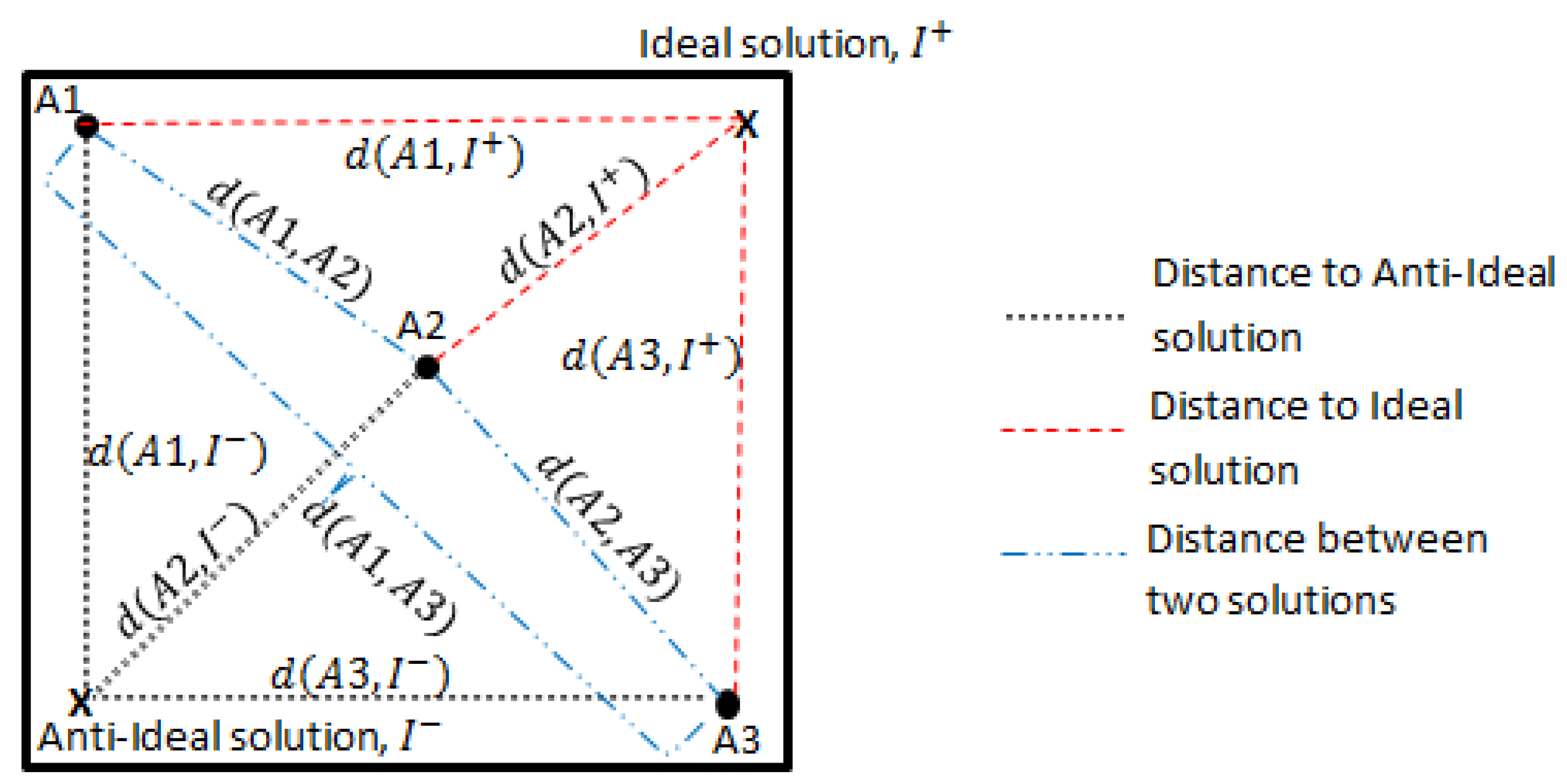
The concepts of distance measure in TOPSIS and the trade-off ranking method are illustrated in Figure 3.
Figure 3 shows the difference in the distance measure between TOPSIS and the trade-off ranking method in evaluating three Pareto alternatives and . TOPSIS uses the distance between an alternative to the ideal/anti-ideal solutions as a ranking measure, which are denoted in Figure 3 as and , respectively, for . In turn, the trade-off ranking method uses the distance between an alternative to the extreme solutions or other alternatives to determine the ranking. In Figure 3, such distances are marked as and . The ranking determination in the trade-off ranking method depends on the sum of the distances between those alternatives. The example in Figure 3 also shows that alternative , which is the closest to the ideal solution, is also the closest to the anti-ideal solution compared to alternatives and . In this case, the property of the TOPSIS method to have the best solution as the closest to the ideal solution and the farthest to the anti-ideal solution is violated.
3.2. Fuzzy Trade-Off Ranking Method
Another way to solve the fuzzy MCDM problem is using the fuzzy MCDM method. In this approach, the fuzzy numbers are processed until the end of the algorithms. As such, the fuzzy information is preserved and the final solution is more accurate. In a fuzzy MCDM method, the distance formula between fuzzy numbers (11) is used for the ranking determination. An algorithm for the fuzzy trade-off ranking (FTOR) method is presented in the following steps:
- Normalization of the performance of criterion j in alternative i,, by equation:where The operator ⊖ is the subtraction of the fuzzy numbers such as Equation (5). The result of the normalized performance is denoted as a triangular fuzzy number
- Determination of the extreme solutions, , by formula:
- Calculation of the distance of an alternative to an extreme solution , denoted as , using equation:The distance between two fuzzy numbers, , is calculated using Equation (11).
- Calculation of the first level of fuzzy trade-off, which is the trade-off between an alternative with all the extreme solutions, is given by formula:whereHere, is defuzzified using Equation (12). In turn, is the weight of each criterion in the fuzzy MCDM problem, presented by a triangular fuzzy number , . Similarly to , the alternative with the least is regarded as the best option. Again, in the case of the same value, the fuzzy trade-off ranking formulation is imposed further, as shown in Step 5 onwards.
- Calculation of the distance of an alternative to the other alternatives is determined by the formula:where . The multiplication of two fuzzy numbers is calculated using Equation (6), while is the distance between two fuzzy numbers determined by Formula (11). The distance calculation represents the total trade-off in the quantity of each criterion. Hence, the least distance value denotes the least trade-off between the two alternatives.
- Calculation of the second level of fuzzy trade-off, which is the trade-off among the alternatives, is given by equation:The degree of fuzzy trade-off represents the sum of distances between one alternative and all the other alternatives in a fuzzy environment. The least value of denotes the least value of compromise between the alternatives. Therefore, the best alternative in the fuzzy trade-off ranking contains the lowest value of if is the same.
4. Numerical Example: Personnel Selection Problem
Consider a numerical example of the personnel selection problem where five benefit criteria are considered in selecting one of three candidates, , for the post of system analysis engineer [30]. The criteria considered are stated as follows:
- Emotional steadiness, ;
- Oral communication skill, ;
- Personality, ;
- Past experience, ;
- Self-confidence, .
Here, the fuzzy trade-off ranking, fuzzy TOPSIS and fuzzy VIKOR methods are used to solve the personnel selection problem. Suppose the rating process of each alternative and the weight of each criterion are made by three DMs. The results of the rating evaluations are shown in Table 3 and Table 4. The rating value is described by the linguistic terms expressed in the triangular fuzzy numbers as seen in Table 1 and Table 2.
Formulae (1) and (2) are applied to the data in Table 3 and Table 4, respectively, in order to find the average performance of the alternative and the average weight of each criterion. The fuzzy decision matrix of the problem is then given in Table 5.
The defuzzified decision matrix using Formula (12) is given in Table 6.
This problem aims to maximize all the criteria. However, the conflicting situation arises since none of the candidates possessed the best in all criteria. More details can be seen in Table 6. According to Table 6, candidate is ranked second in criteria , , and . Meanwhile, candidate is ranked first in criterion . Furthermore, candidate is ranked first out of two criteria, which are and , but ranked third in two other criteria, and . Meanwhile, candidate is ranked the best in two criteria, and , but the worst in three other criteria, which are , and .
The normalized defuzzified decision matrix by the trade-off ranking method, Formula (13), is given in Table 7.
Referring to Table 7 and using Formula (14), the extreme solutions for the trade-off ranking method are determined. As an example, an alternative with the optimal value in criterion is the fifth extreme solution for the problem, i.e., since .
After calculating the data in Table 7, using Formulae (15) and (16), and the data in Table 5 with Formulae (17) and (18), the ranking by the trade-off method with defuzzification and the fuzzy trade-off ranking are given in Table 8. As can be observed in Table 8, the best candidate ranked by the fuzzy trade-off is candidate . In addition, it is also the best candidate ranked by the pre-defuzzification approach in the trade-off ranking method. Note that, even though candidate is only ranked first in one criterion, he/she is not ranked the worst in the other criteria. Thus, this candidate has the most balanced traits, i.e., the least compromise, out of all five criteria compared to and .
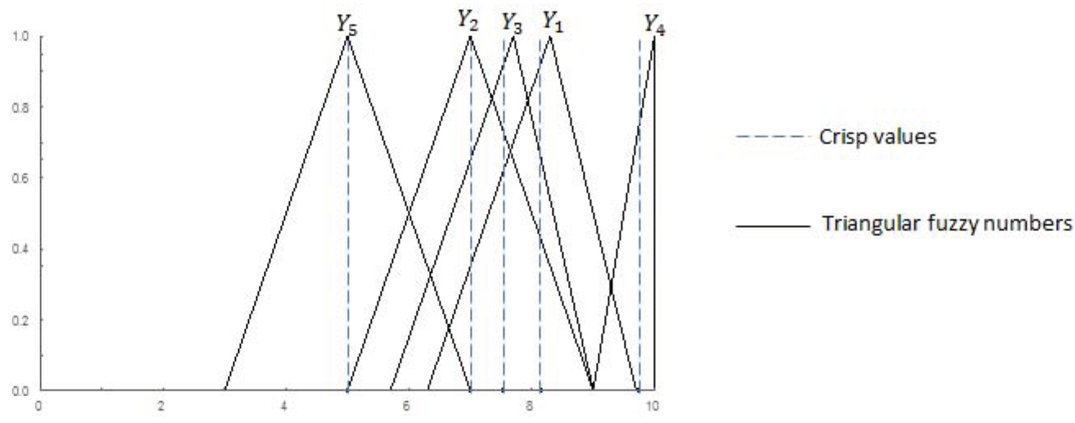
Table 9 shows the results of the fuzzy trade-off and the defuzzification trade-off . The indifference in the ranking by the trade-off method with defuzzification and the fuzzy trade-off ranking method is due to the small range of fuzziness in the triangular fuzzy numbers and small differences in the criteria ratings. The crisp values of the fuzzy numbers given in Table 6 significantly close to their middle values, , presented in Table 5. A graphical explanation for this statement is given in Figure 4.
The triangular fuzzy numbers of each criterion for alternative and their respective crisp values are shown in Figure 4. As can be seen, the crisp values are situated close to the middle values of the triangular fuzzy numbers. Hence, there is a small difference in the and values for each alternative and indifference in the ranking solutions. In the fuzzy MCDM problem, the final result is a crisp value since the MCDM method must provide a deterministic solution.
Next, consider the ranking by fuzzy VIKOR as given in Table 10. The fuzzy ranking in the fuzzy VIKOR method gives a partial ranking since the first position in is not confirmed (Step 5 in Section 2.4).
In the case of ranking by VIKOR defuzzification, the final decision is the set of compromise solutions {, , } (Step 8 in Section 2.4). Eventually, since there are only three options, the defuzzification ranking by VIKOR gives a set of solutions with all three options. The results obtained by the fuzzy VIKOR are given in Table 11.
Next, the ranking by the fuzzy TOPSIS is given in Table 12. This method also identifies candidate as the best candidate.
As can be seen from Table 12, alternative is the closest to the ideal solution (). However, it is not the farthest from the anti-ideal solution (). In fact, the alternative farthest from the anti-ideal solution is (). It shows that the concept of the TOPSIS method, to have the best solution that is the closest to the ideal and the farthest from the anti-ideal solutions, is not realized in this conflicting multi-criteria problem.
Now, suppose the DM have changed their preferences towards each criterion. The new DM’s preferences, presented by the linguistic variables, are given in Table 13. According to Table 1, as well as Formulae (2) and (12), the fuzzy and defuzzified weights associated with the new preferences are shown in Table 14.
As can be seen from Table 14, the DM now prefer criterion (emotional steadiness) and criterion (past experience) more than the other criteria. The results by each fuzzy MCDM method for the new criteria weights are given in Table 15.
From the results in Table 15, the best candidate by the fuzzy trade-off ranking method is candidate . Note that candidate is ranked the lowest with the previous criteria weights. The difference is related to DM’s preferences. In the previous problem, DM’s preferences towards each criterion are quite equal (Table 7). However, in the new weights problem, the DM prefer criteria and more than the others. According to Table 7, candidate possesses the best score in both criteria preferred by the DMs. Hence, it is now regarded as the best choice. In turn, the worst candidate is since this candidate is ranked the lowest in both criteria and .
Meanwhile, the fuzzy VIKOR method gives a set of compromise solutions as a final ranking result for the new weights case. As for the fuzzy TOPSIS, the best option for the new weights is the same as in the previous weights case, i.e., candidate . The difference now is in the results such that the alternative that is closer to the ideal solution () is also farther from the anti-ideal solution ().
5. Conclusions
A fuzzy trade-off ranking method for the fuzzy MCDM problem has been proposed. The approach has been utilised to find the best solution to the fuzzy conflicting multi-criteria problem. The fuzzy trade-off ranking method is able to capture the solution with the least compromise. It is also able to comprehend DM’s preferences in a conflicting MCDM problem. The algorithm takes into account the position of an alternative with respect to the other alternatives. Therefore, in contrast to other techniques, the ranking analysis is nonlocal. The proposed methodology has been compared against two well known fuzzy methods, VIKOR and TOPSIS, in application to the personnel selection problem.
In contrast to the fuzzy trade-off ranking method, the fuzzy TOPSIS method is an individual performance method, where an alternative is only compared against the ideal/anti-ideal solutions, which are artificial solutions. Such a ranking calculation is the best for the MCDM problem, where an alternative that is close to the ideal solution is also far from the anti-ideal solution. However, in a conflicting MCDM problem, such an assumption is not always realized. The best solution that is the closest to the ideal solution may not be the farthest from the anti-ideal solution. On the contrary, the fuzzy VIKOR gives a similar solution as the fuzzy trade-off ranking since the fuzzy VIKOR was also developed to tackle the conflicting MCDM problems. However, in some problems, as shown in the numerical example, the fuzzy VIKOR gives a set of compromise solutions rather than one single solution. In that matter, the DM still has to choose one solution out of the compromise set proposed by the fuzzy VIKOR method. In future work, the approach will be applied to a wider range of data including continuous, ordinal and categorical variables. More practical problems will be considered. Comparisons with other available ranking techniques are also needed. The final selection of the ranking method depends on the preferences of the Decision-Maker. Systematic comparison of the available techniques for different classes of problems should be valuable.
Supplementary Materials
Supplementary File 1Acknowledgments
The first author gratefully acknowledges the research scholarship awarded by the Ministry of Higher Education Malaysia and the University of Malaysia Pahang. The authors are grateful to unknown references for valuable remarks that essentially improved the quality of the paper.
Author Contributions
Nor Izzati Jaini designed and performed the numerical experiments, and Sergei V. Utyuzhnikov designed the algorithm; the contribution of the authors to the other work was equal.
Conflicts of Interest
The authors declare no conflict of interest.
References
- Eckenrode, R.T. Weighting Multiple Criteria. Manag. Sci. 1965, 12, 180–192. [Google Scholar] [CrossRef]
- Saaty, T.L. The Analytic Hierarchy Process: Planning, Priority Setting, Resources Allocation; McGraw: New York, NY, USA, 1980. [Google Scholar]
- Kablan, M.M. Decision support for energy conservation promotion: An analytic hierarchy process approach. Energy Policy 2004, 32, 1151–1158. [Google Scholar] [CrossRef]
- Iwanejko, R. Multicriterion AHP decision-making model as a tool for supporting the selection of optimal decision in a water supply system. Environ. Prot. Eng. 2007, 33, 141–146. [Google Scholar]
- Wu, C.R.; Lin, C.T.; Chen, H.C. Optimal selection of location for Taiwanese hospitals to ensure a competitive advantage by using the analytic hierarchy process and sensitivity analysis. Build. Environ. 2007, 42, 1431–1444. [Google Scholar] [CrossRef]
- Contreras, F.; Hanaki, K.; Aramaki, T.; Connors, S. Application of analytical hierarchy process to analyze stakeholders preferences for municipal solid waste management plans, Boston, USA. Resour. Conserv. Recycl. 2008, 52, 979–991. [Google Scholar] [CrossRef]
- Chatzimouraddis, A.I.; Pilavachi, P.A. Technological, economic and sustainability evaluation of power plants using the Analytic Hierarchy Process. Energy Policy 2009, 37, 778–787. [Google Scholar] [CrossRef]
- Zaidan, A.A.; Zaidan, B.B.; Hussain, M.; Haiqi, A.; Kiah, M.M.; Abdulnabi, M. Multi-criteria analysis for OS-EMR software selection problem: A comparative study. Decis. Support Syst. 2015, 78, 15–27. [Google Scholar] [CrossRef]
- Saaty, T.L. The Analytic Network Process-Decision-Making with Dependence and Feedback; RWS Publications: Pittsburgh, PA, USA, 1996. [Google Scholar]
- Levy, J.K. Multiple criteria decision-making and decision support systems for flood risk management. Stoch. Environ. Res. Risk Assess. 2005, 19, 438–447. [Google Scholar] [CrossRef]
- Khan, S.; Faisal, M.N. An analytic network process model for municipal solid waste disposal options. Waste Manag. 2008, 28, 1500–1508. [Google Scholar] [CrossRef] [PubMed]
- Gomez-Navarro, T.; Garcia-Melon, M.; Acuna-Dutra, S.; Diaz-Martin, D. An environmental pressure index proposal for urban development planning based on the analytic network process. Environ. Impact Assess. Rev. 2009, 29, 319–329. [Google Scholar] [CrossRef]
- Boj, J.J.; Rodriguez-Rodriguez, R.; Alfaro-Saiz, J.J. An ANP-multi-criteria-based methodology to link intangible assets and organizational performance in a Balanced Scorecard context. Decis. Support Syst. 2014, 68, 98–110. [Google Scholar] [CrossRef]
- Keeney, R.L.; Raiffa, H. Decisions with Multiple Objectives: Preferences and Value Trade-offs; Wiley: New York, NY, USA, 1976. [Google Scholar]
- Ananda, J.; Herath, G. Evaluating public risk preferences in forest land-use choices using multi-attribute utility theory. Ecol. Econ. 2005, 55, 408–419. [Google Scholar] [CrossRef]
- Brans, J.; Vincke, P. A preference ranking organisation method: The PROMETHEE method for MCDM. Manag. Sci. 1985, 31, 647–656. [Google Scholar] [CrossRef]
- Goumas, M.; Lygerou, V. An extension of the PROMETHEE method for decision-making in fuzzy environment: Ranking of alternative energy exploitation projects. Eur. J. Oper. Res. 2000, 123, 606–613. [Google Scholar] [CrossRef]
- Oberschmidt, J.; Geldermann, J.; Ludwig, J.; Schmehl, M. Modified PROMETHEE approach for assessing energy technologies. Int. J. Energy Sect. Manag. 2010, 4, 183–212. [Google Scholar] [CrossRef]
- Petrović, M.; Bojković, N.; Anić, I.; Stamenković, M.; Tarle, S.P. An ELECTRE-based decision aid tool for stepwise benchmarking: An application over EU Digital Agenda targets. Decis. Support Syst. 2014, 59, 230–241. [Google Scholar] [CrossRef]
- Fonseca, C.M.; Fleming, P.J. Genetic Algorithms for Multiobjective Optimization: Formulation, Discussion and Generalization. Int. Comput. Games Assoc. 1993, 93, 416–423. [Google Scholar]
- Tanaka, M.; Watanabe, H.; Furukawa, Y.; Tanino, T. GA-based decision support system for multicriteria optimization. In Proceedings of the IEEE International Conference on Intelligent Systems for the 21st Century, Systems, Man and Cybernetics, Vancouver, BC, Canada, 22–25 October 1995; Volume 2, pp. 1556–1561. [Google Scholar]
- Feng, C.W.; Liu, L.; Burns, S.A. Using genetic algorithms to solve construction time-cost trade-off problems. J. Comput. Civ. Eng. 1997, 11, 184–189. [Google Scholar] [CrossRef]
- Hegazy, T. Optimization of construction time-cost trade-off analysis using genetic algorithms. Can. J. Civ. Eng. 1999, 26, 685–697. [Google Scholar] [CrossRef]
- Zheng, D.X.; Ng, S.T.; Kumaraswamy, M.M. Applying Pareto ranking and niche formation to genetic algorithm-based multiobjective time-cost optimization. J. Constr. Eng. Manag. 2005, 131, 81–91. [Google Scholar] [CrossRef]
- Wang, Y.; Yang, Y. Particle swarm optimization with preference order ranking for multi-objective optimization. Inf. Sci. 2009, 179, 1944–1959. [Google Scholar] [CrossRef]
- Hwang, C.L.; Yoon, K. Multiple Attribute Decision-Making: Methods and Applications, A State of the Art Survey; Springer: New York, NY, USA, 1981. [Google Scholar]
- Opricovic, S.; Tzeng, G.H. Compromise solution by MCDM methods: A comparative analysis of VIKOR and TOPSIS. Eur. J. Oper. Res. 2004, 156, 445–455. [Google Scholar] [CrossRef]
- Wang, J.W.; Cheng, C.H.; Huang, K.C. Fuzzy hierarchical TOPSIS for supplier selection. Appl. Soft Comput. 2009, 9, 377–386. [Google Scholar] [CrossRef]
- Kao, C. Weight determination for consistently ranking alternatives in multiple criteria decision analysis. Appl. Math. Model. 2010, 34, 1779–1787. [Google Scholar] [CrossRef]
- Chen, C.T. Extensions of the TOPSIS for group decision-making under fuzzy environment. Fuzzy Sets Syst. 2000, 114, 1–9. [Google Scholar] [CrossRef]
- Jahanshahloo, G.R.; Lotfi, F.H.; Izadikhah, M. An algorithmic method to extend TOPSIS for decision-making problems with interval data. Appl. Math. Comput. 2006, 175, 1375–1384. [Google Scholar] [CrossRef]
- Wang, T.C.; Chang, T.H. Application of TOPSIS in evaluating initial training aircraft under a fuzzy environment. Expert Syst. Appl. 2007, 33, 870–880. [Google Scholar] [CrossRef]
- Gumus, A.T. Evaluation of hazardous waste transportation firms by using a two-step fuzzy-AHP and TOPSIS methodology. Expert Syst. Appl. 2009, 36, 4067–4074. [Google Scholar] [CrossRef]
- Zadeh, L.A. Fuzzy sets. Inf. Control 1965, 8, 338–353. [Google Scholar] [CrossRef]
- Cakir, O.; Canbolat, M.S. A web-based decision support system for multi-criteria inventory classification using fuzzy AHP methodology. Expert Syst. Appl. 2008, 35, 1367–1378. [Google Scholar] [CrossRef]
- Gungor, Z.; Serhadlioglu, G.; Kesen, S.E. A fuzzy AHP approach to personnel selection problem. Appl. Soft Comput. 2009, 9, 641–646. [Google Scholar] [CrossRef]
- Amiri, M.P. Project selection for ooil-field development by using the AHP and fuzzy TOPSIS methods. Expert Syst. Appl. 2010, 37, 6218–6224. [Google Scholar] [CrossRef]
- Buyukozkan, G.; Cifci, G.; Guleryuz, S. Strategic analysis of healhealth service quality using fuzzy AHP methodology. Expert Syst. Appl. 2011, 38, 9407–9424. [Google Scholar] [CrossRef]
- Kilincci, O.; Onal, S.A. Fuzzy AHP approach for supplier selection in a washing machine company. Expert Syst. Appl. 2011, 38, 9656–9664. [Google Scholar] [CrossRef]
- Torlak, G.; Sevkli, M.; Sanal, M.; Zaim, S. Analyzing business competition by using fuzzy TOPSIS method: An example of Turkish domestic airline industry. Expert Syst. Appl. 2011, 38, 3396–3406. [Google Scholar] [CrossRef]
- Buyukozkan, G.; Cifci, G. A combined fuzzy AHP and fuzzy TOPSIS based strategic analysis of electronic service quality in healhealth industry. Expert Syst. Appl. 2012, 39, 2341–2354. [Google Scholar] [CrossRef]
- Rouhani, S.; Ghazanfari, M.; Jafari, M. Evaluation model of business intelligence for enterprise systems using fuzzy TOPSIS. Expert Syst. Appl. 2012, 39, 3764–3771. [Google Scholar] [CrossRef]
- Perny, P.; Roubens, M. Fuzzy preference modeling. In Fuzzy Sets in Decision Analysis, Operations Research and Statistics; Springer: Berlin, Germany, 1998; pp. 3–30. [Google Scholar]
- Esmaeilpour, M.; Mohammadi, A.R.A. Analyzing the EEG signals in order to estimate the depth of anesthesia using wavelet and fuzzy neural networks. Int. J. Interact. Multimedia Artif. Intell. 2015, 4, 12–15. [Google Scholar] [CrossRef]
- Taibi, A.; Atmani, B. Combining fuzzy AHP with GIS and decision rules for industrial site selection. Int. J. Interact. Multimedia Artif. Intell. 2017, 4, 60–69. [Google Scholar] [CrossRef]
- Runkler, T.; Coupland, S.; John, R. Interval type-2 fuzzy decision-making. Int. J. Approx. Reason. 2017, 80, 217–224. [Google Scholar] [CrossRef]
- Van Leekwijck, W.; Kerre, E.E. Defuzzification: Criteria and classification. Fuzzy Sets Syst. 1999, 108, 159–178. [Google Scholar] [CrossRef]
- Wang, W.J.; Luoh, L. Simple computation for the defuzzifications of center of sum and center of gravity. J. Intell. Fuzzy Syst. 2000, 9, 53–59. [Google Scholar]
- Wang, Y.M.; Elhag, T.M. Fuzzy TOPSIS method based on alpha level sets with an application to bridge risk assessment. Expert Syst. Appl. 2006, 31, 309–319. [Google Scholar] [CrossRef]
- Wang, Y.J.; Lee, H.S. Generalizing TOPSIS for fuzzy multiple-criteria group decision-making. Comput. Math. Appl. 2007, 53, 1762–1772. [Google Scholar] [CrossRef]
- Krohling, R.A.; Campanharo, V.C. Fuzzy TOPSIS for group decision-making: A case study for accidents with oil spill in the sea. Expert Syst. Appl. 2011, 38, 4190–4197. [Google Scholar] [CrossRef]
- Opricovic, S. A fuzzy compromise solution for multicriteria problems. Int. J. Uncertain. Fuzziness Knowl.-Based Syst. 2007, 15, 363–380. [Google Scholar] [CrossRef]
- Opricovic, S. Fuzzy VIKOR with an application to water resources planning. Expert Syst. Appl. 2011, 38, 12983–12990. [Google Scholar] [CrossRef]
- Yurdakul, M.; Iç, Y.T. Analysis of the benefit generated by using fuzzy numbermethodsTOPSIS model developed for machine tool selection problems. J. Mater. Process. Technol. 2009, 209, 310–317. [Google Scholar] [CrossRef]
- Zouggari, A.; Benyoucef, L. Simulation based fuzzy TOPSIS approach for group multi-criteria supplier selection problem. Eng. Appl. Artif. Intell. 2012, 25, 507–519. [Google Scholar] [CrossRef]
- Rouyendegh, B.D.; Saputro, T.E. Supplier selection using integrated fuzzy TOPSIS and MCGP: A case study. Procedia Soc. Behav. Sci. 2014, 116, 3957–3970. [Google Scholar] [CrossRef]
- Ertuğrul, İ.; Karakaşoğlu, N. Performance evaluation of Turkish cement firms with fuzzy analytic hierarchy process and TOPSIS methods. Expert Syst. Appl. 2009, 36, 702–715. [Google Scholar] [CrossRef]
- Sun, C.C.; Lin, G.T. Using fuzzy TOPSIS method for evaluating the competitive advantage of shopping websites. Expert Syst. Appl. 2009, 36, 11764–11771. [Google Scholar] [CrossRef]
- Sun, C.C. A performance evaluation model by integrating fuzzy AHP and fuzzy TOPSIS methods. Expert Syst. Appl. 2010, 37, 7745–7754. [Google Scholar] [CrossRef]
- Yu, X.; Guo, S.; Guo, J.; Huang, X. Rank B2C e-commerce websites in e-alliance based on AHP and fuzzy TOPSIS. Expert Syst. Appl. 2011, 38, 3550–3557. [Google Scholar] [CrossRef]
- Wu, H.Y.; Tzeng, G.H.; Chen, Y.H. A fuzzy MCDM approach for evaluating banking performance based on Balanced Scorecard. Expert Syst. Appl. 2009, 36, 10135–10147. [Google Scholar] [CrossRef]
- Wu, H.Y.; Chen, J.K.; Chen, I.S. Innovation capital indicator assessment of Taiwanese Universities: A hybrid fuzzy model application. Expert Syst. Appl. 2010, 37, 1635–1642. [Google Scholar] [CrossRef]
- Jaini, N.; Utyuzhnikov, S. Trade-off Ranking Method for Multi-Criteria Decision Analysis. Multi-Criteria Decis. Anal. 2017, 24, 121–132. [Google Scholar] [CrossRef]
- Zadeh, L.A. The concept of a linguistic variable and its application to approximate reasoning I. Inf. Sci. 1975, 8, 199–249. [Google Scholar] [CrossRef]
- Zadeh, L.A. The concept of a linguistic variable and its application to approximate reasoning II. Inf. Sci. 1975, 8, 301–357. [Google Scholar] [CrossRef]
- Sodhi, B.; Tadinada, P. A Simplified Description of Fuzzy TOPSIS. arXiv, 2012; arXiv:1205.5098. [Google Scholar]
- Klir, G.; Yuan, B. Fuzzy Sets and Fuzzy Logic; Prentice Hall: Upper Saddle River, NJ, USA, 1995; Volume 4. [Google Scholar]
- Giachetti, R.E.; Young, R.E. A parametric representation of fuzzy numbers and their arithmetic operators. Fuzzy Sets Syst. 1997, 91, 185–202. [Google Scholar] [CrossRef]
- Chiu, C.H.; Wang, W.J. A simple computation of MIN and MAX operations for fuzzy numbers. Fuzzy Sets Syst. 2002, 126, 273–276. [Google Scholar] [CrossRef]
- Erfani, T.; Utyuzhnikov, S.V. Directed search domain: A method for even generation of the Pareto frontier in multiobjective optimization. Eng. Optim. 2011, 43, 467–484. [Google Scholar] [CrossRef]
Figure 1.
Membership functions of the linguistic variables.
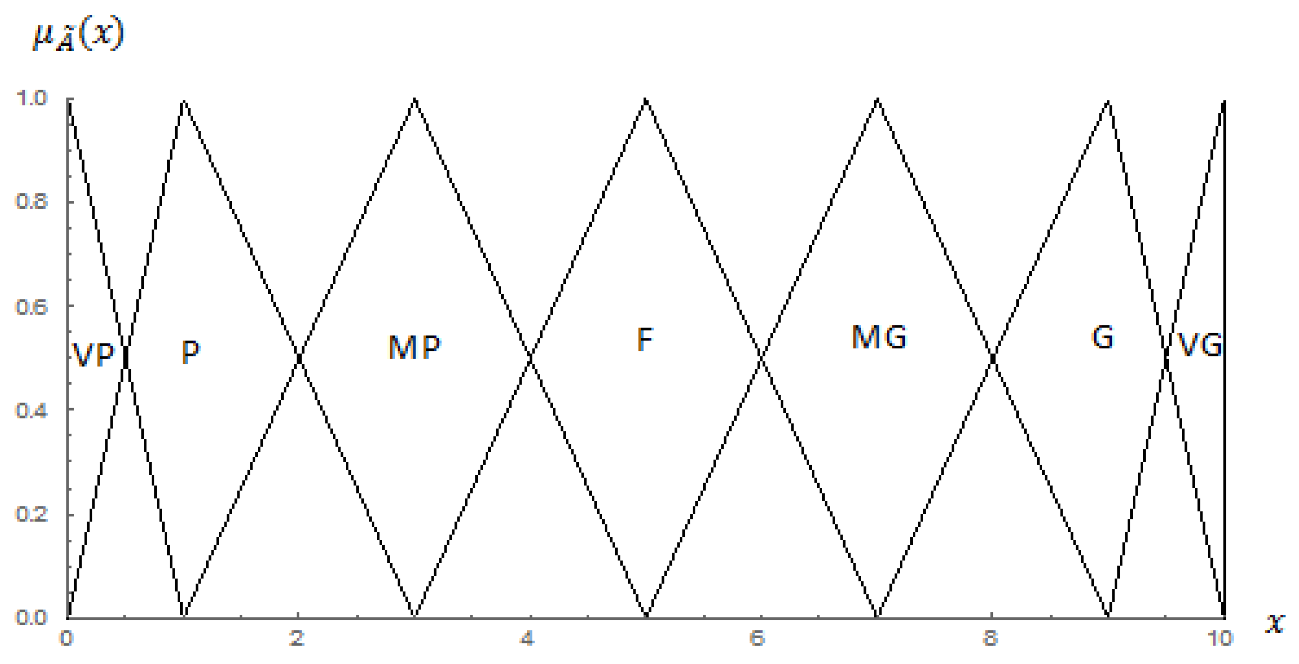
Figure 2.
Triangular fuzzy number .

Figure 3.
Distance measurement in TOPSIS and trade-off ranking.

Figure 4.
Triangular fuzzy numbers and their crisp values of each criterion for alternative .


Table 1.
Fuzzy numbers for the importance weight of each criterion.
| Meaning of Linguistic Scale | Numerical Scale |
|---|---|
| Very low (VL) | (0, 0, 0.1) |
| Low (L) | (0, 0.1, 0.3) |
| Medium low (ML) | (0.1, 0.3, 0.5) |
| Medium (M) | (0.3, 0.5, 0.7) |
| Medium high (MH) | (0.5, 0.7, 0.9) |
| High (H) | (0.7, 0.9, 1.0) |
| Very high (VH) | (0.9, 1.0, 1.0) |
Table 2.
Linguistic variables for the alternative performance.
| Meaning of Linguistic Scale | Numerical Scale |
|---|---|
| Very poor (VP) | (0, 0, 1) |
| Poor (P) | (0, 1, 3) |
| Medium poor (MP) | (1, 3, 5) |
| Fair (F) | (3, 5, 7) |
| Medium good (MG) | (5, 7, 9) |
| Good (G) | (7, 9, 10) |
| Very good (VG) | (9, 10, 10) |
Table 3.
Criteria weightage by decision-makers.
| Criterion | |||
|---|---|---|---|
| H | H | H | |
| VH | VH | VH | |
| VH | H | H | |
| VH | VH | VH | |
| M | MH | MH |
Table 4.
Alternatives ratings by decision-makers.
| Criterion | |||||||||
|---|---|---|---|---|---|---|---|---|---|
| MG | G | MG | G | G | MG | VG | G | F | |
| VG | VG | VG | MG | MG | MG | G | G | G | |
| G | G | G | F | G | G | VG | VG | G | |
| G | G | G | VG | VG | VG | VG | G | VG | |
| G | G | G | F | F | F | G | G | MG | |
Table 5.
The fuzzy decision matrix for the personnel selection problem.
| Weight | |||||
|---|---|---|---|---|---|
| (0.7,0.9,1) | (0.9,1,1) | (0.77,0.93,1) | (0.9,1,1) | (0.43,0.63,0.83) | |
| (5.7,7.7,9.3) | (9,10,10) | (7,9,10) | (7,9,10) | (7,9,10) | |
| (6.3,8.3,9.7) | (5,7,9) | (5.7,7.7,9) | (9,10,10) | (3,5,7) | |
| (6.3,8,9) | (7,9,10) | (8.3,9.7,10) | (8.3,9.7,10) | (6.3,8.3,9.7) |
Table 6.
Defuzzified decision matrix.
| Weight | |||||
|---|---|---|---|---|---|
| 0.875 | 0.975 | 0.908 | 0.975 | 0.630 | |
| 7.60 | 9.75 | 8.75 | 8.75 | 8.75 | |
| 8.15 | 7.00 | 7.53 | 9.75 | 5.00 | |
| 7.83 | 8.75 | 9.43 | 9.42 | 8.15 |
Table 7.
Normalized defuzzified decision matrix by the trade-off ranking.
| Weight | |||||
|---|---|---|---|---|---|
| 0.201 | 0.223 | 0.208 | 0.223 | 0.144 | |
| 0 | 1 | 0.64 | 0 | 1 | |
| 1 | 0 | 0 | 1 | 0 | |
| 0.42 | 0.64 | 1 | 0.68 | 0.84 |
Table 8.
Ranking by fuzzy trade-off.
| Ranking | 1 | 2 | 3 |
|---|---|---|---|
| Fuzzy trade-off | |||
| Defuzzification |
Table 9.
Results by fuzzy trade-off.
| Trade-Off | |||
|---|---|---|---|
| 1.027 | 1.039 | 0.984 | |
| 1.090 | 1.105 | 1.030 |
DT1 is first level trade-off; DFT1, fuzzy DT1.
Table 10.
Ranking by fuzzy VIKOR.
| Ordering | 1 | 2 | 3 | |
|---|---|---|---|---|
| Defuzzification | ||||
Table 11.
Results by fuzzy VIKOR.
| 0.62 | 1.39 | 0.43 | ||
| 3.25 | 4.01 | 2.85 | ||
| Crisp | 0.75 | 1.44 | 0.57 | |
| 0 | ||||
| 0.33 | 0.6 | 0.2 | ||
| 1 | 1 | 0.85 | ||
| Crisp | 0.37 | 0.55 | 0.27 | |
| 0 | 0.11 | 0.01 | ||
| 0.066 | 0.24 | 0 | ||
| 0.095 | 0.18 | 0 | ||
| Crisp | 0.057 | 0.193 | 0.003 |
Table 12.
Ranking and results by fuzzy TOPSIS.
| Ranking | 1 | 2 | 3 |
|---|---|---|---|
| 1.45 | 1.48 | 1.87 | |
| 3.93 | 3.95 | 3.52 | |
| 0.731 | 0.728 | 0.653 |
Table 13.
New criteria weightage by decision makers.
| Criterion | |||
|---|---|---|---|
| MH | H | H | |
| VL | L | VL | |
| ML | ML | ML | |
| H | H | VH | |
| L | VL | L |
Table 14.
New fuzzy and defuzzified weights.
| (0.63,0.83,0.97) | (0,0.03,0.17) | (0.1,0.3,0.5) | (0.77,0.93,1) | (0,0.07,0.23) | |
| 0.82 | 0.06 | 0.3 | 0.91 | 0.09 |
Table 15.
Results by the fuzzy MCDM methods with the new criteria weights.
| MCDM Method | |||
|---|---|---|---|
| Fuzzy Trade-off | |||
| 1.700 | 0.354 | 1.272 | |
| 1.799 | 0.364 | 1.334 | |
| Fuzzy VIKOR | |||
| Crisp | 0.662 | 0.411 | 0.357 |
| Crisp | 0.405 | 0.276 | 0.253 |
| 0.007 | 0 | 0.016 | |
| 0.145 | 0.024 | 0 | |
| 0.188 | 0.045 | 0 | |
| Crisp | 0.121 | 0.023 | 0.004 |
| Fuzzy TOPSIS | |||
| 3.283 | 3.215 | 3.184 | |
| 2.074 | 2.096 | 2.125 | |
| 0.387 | 0.395 | 0.400 |
© 2017 by the authors. Licensee MDPI, Basel, Switzerland. This article is an open access article distributed under the terms and conditions of the Creative Commons Attribution (CC BY) license (http://creativecommons.org/licenses/by/4.0/).
Share and Cite
MDPI and ACS Style
Jaini, N.I.; Utyuzhnikov, S.V. A Fuzzy Trade-Off Ranking Method for Multi-Criteria Decision-Making. Axioms 2018, 7, 1. https://doi.org/10.3390/axioms7010001
AMA Style
Jaini NI, Utyuzhnikov SV. A Fuzzy Trade-Off Ranking Method for Multi-Criteria Decision-Making. Axioms. 2018; 7(1):1. https://doi.org/10.3390/axioms7010001
Chicago/Turabian StyleJaini, Nor Izzati, and Sergey V. Utyuzhnikov. 2018. "A Fuzzy Trade-Off Ranking Method for Multi-Criteria Decision-Making" Axioms 7, no. 1: 1. https://doi.org/10.3390/axioms7010001
Note that from the first issue of 2016, this journal uses article numbers instead of page numbers. See further details here.