NN-Harmonic Mean Aggregation Operators-Based MCGDM Strategy in a Neutrosophic Number Environment


1
Department of Mathematics, Jadavpur University, Kolkata-700032 West Bengal, India
2
Department of Mathematics, Nandalal Ghosh B.T. College, Panpur, PO-Narayanpur, and District: North 24 Parganas, Pin-743126 West Bengal, India
3
Mathematics & Science Department, University of New Mexico, 705 Gurley Ave., Gallup, NM 87301, USA
*
Author to whom correspondence should be addressed.
Axioms 2018, 7(1), 12; https://doi.org/10.3390/axioms7010012
Submission received: 18 November 2017
/
Revised: 9 February 2018
/
Accepted: 11 February 2018
/
Published: 23 February 2018
(This article belongs to the Special Issue Neutrosophic Multi-Criteria Decision Making)
Abstract
:A neutrosophic number (a + bI) is a significant mathematical tool to deal with indeterminate and incomplete information which exists generally in real-world problems, where a and bI denote the determinate component and indeterminate component, respectively. We define score functions and accuracy functions for ranking neutrosophic numbers. We then define a cosine function to determine the unknown weight of the criteria. We define the neutrosophic number harmonic mean operators and prove their basic properties. Then, we develop two novel multi-criteria group decision-making (MCGDM) strategies using the proposed aggregation operators. We solve a numerical example to demonstrate the feasibility, applicability, and effectiveness of the two proposed strategies. Sensitivity analysis with the variation of “I” on neutrosophic numbers is performed to demonstrate how the preference ranking order of alternatives is sensitive to the change of “I”. The efficiency of the developed strategies is ascertained by comparing the results obtained from the proposed strategies with the results obtained from the existing strategies in the literature.

1. Introduction
Multi-criteria decision-making (MCDM), and multi-criteria group decision-making (MCGDM) are significant branches of decision theories which have been commonly applied in many scientific fields. They have been developed in many directions, such as crisp environments [1,2], and uncertain environments, namely fuzzy environments [3,4,5,6,7,8,9,10,11,12,13], intuitionistic fuzzy environments [14,15,16,17,18,19,20,21,22,23,24], and neutrosophic set environments [25,26,27,28,29,30,31,32,33,34,35,36,37,38,39,40,41,42,43,44,45]. Smarandache [46,47] introduced another direction of uncertainty by defining neutrosophic numbers (NN), which represent indeterminate and incomplete information in a new way. A NN consists of a determinate component and an indeterminate component. Thus, the NNs are more applicable to deal with indeterminate and incomplete information in real world problems. The NN is expressed as the function N = p + qI in which p is the determinate component and qI is the indeterminate component. If N = qI, i.e., the indeterminate part reaches the maximum label, the worst situation occurs. If N = p, i.e., the indeterminate part does not appear, the best situation occurs. Thus, the application of NNs is more appropriate to deal with the indeterminate and incomplete information in real-world decision-making situations.
Information aggregation is an essential practice of accumulating relevant information from various sources. It is used to present aggregation between the min and max operators. The harmonic mean is usually used as a mathematical tool to accumulate the central tendency of information [48].
The harmonic mean (HM) is widely used in statistics to calculate the central tendency of a set of data. Park et al. [49] proposed multi-attribute group decision-making (MAGDM) strategy based on HM operators under uncertain linguistic environments. Wei [50] proposed a MAGDM strategy based on fuzzy-induced, ordered, weighted HM. In a fuzzy environment, Xu [48] studied a fuzzy-weighted HM operator, fuzzy ordered weighted HM operator, and a fuzzy hybrid HM operator, and employed them for MADM problems. Ye [51] proposed a multi-attribute decision-making (MADM) strategy based on harmonic averaging projection for a simplified neutrosophic sets (SNS) environment.
In a NN environment, Ye [52] proposed a MAGDM using de-neutrosophication strategy and a possibility degree ranking strategy for neutrosophic numbers. Liu and Liu [53] proposed a NN generalized weighted power averaging operator for MAGDM. Zheng et al. [54] proposed a MAGDM strategy based on a NN generalized hybrid weighted averaging operator. Pramanik et al. [55] studied a teacher selection strategy based on projection and bidirectional projection measures in a NN environment.
Only four [52,53,54,55] MCGDM strategies using NNs have been reported in the literature. Motivated from the works of Ye [52], Liu and Liu [53], Zheng et al. [54], and Pramanik et al. [55], we consider the proposed strategies to handle MCGDM problems in a NN environment.
The strategies [52,53,54,55] cannot deal with the situation when larger values other than arithmetic mean, geometric mean, and harmonic mean are necessary for experimental purposes. To fill the research gap, we propose two MCGDM strategies.
In this paper, we develop two new MCGDM strategies based on a NN harmonic mean operator (NNHMO) and a NN weighted harmonic mean operator (NNWHMO) to solve MCGDM problems. We define a cosine function to determine unknown weights of the criteria. To develop the proposed strategies, we define score and accuracy functions for ranking NNs for the first time in the literature.
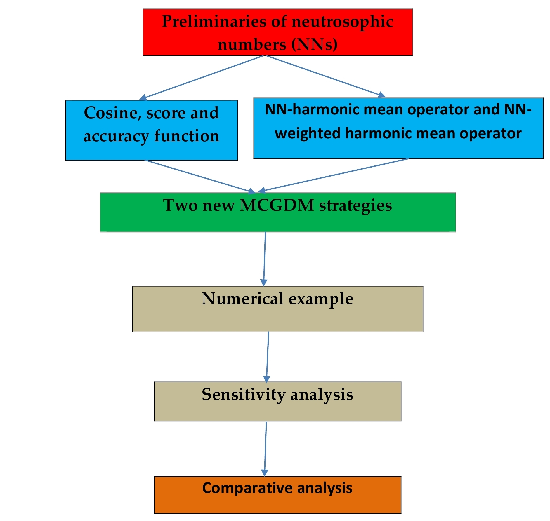
The rest of the paper is structured as follows: Section 2 presents some preliminaries of NNs and score and accuracy functions of NNs. Section 3 devotes NN harmonic mean operator (NNHMO) and NN weighted harmonic mean operator (NNWHMO). Section 4 defines the cosine function to determine unknown criteria weights. Section 5 presents two novel decision-making strategies based on NNHMO and NNWHMO. In Section 6, a numerical example is presented to illustrate the proposed MCGDM strategies and the results show the feasibility of the proposed MCGDM strategies. Section 7 compares the obtained results derived from the proposed strategies and the existing strategies in NN environment. Finally, Section 8 concludes the paper with some remarks and future scope of research.
2. Preliminaries
In this section, definition of harmonic and weighted harmonic mean of positive real numbers, concepts of NNs, operations on NNs, score and accuracy functions of NNs are outlined.
2.1. Harmonic Mean and Weighted Harmonic Mean
Harmonic mean is a traditional average, which is generally used to determine central tendency of data. The harmonic mean is commonly considered as a fusion method of numerical data.
Definition 1.
[48]: The harmonic mean H of the positive real numbers x1, x2, …, xn is defined as: ; i = 1, 2, …, n.
Definition 2.
[49]: The weighted harmonic mean H of the positive real numbers x1, x2, …, xn is defined as ; i = 1, 2, …, n.
Here,
2.2. NNs
A NN [46,47] consists of a determinate component x and an indeterminate component yI, and is mathematically expressed as z = x + yI for x, y R, where I is indeterminacy interval and R is the set of real numbers. A NN z can be specified as a possible interval number, denoted by z = [x + yIL, x + yIU] for z Z (Z is set of all NNs) and I [IL, IU]. The interval I [IL, IU] is considered as an indeterminate interval.
- If yI = 0, then z is degenerated to the determinate component z = x
- If x = 0, then z is degenerated to the indeterminate component z = yI
- If IL = IU, then z is degenerated to a real number.
Let two NNs be z1 = x1 + y1I and z2 = x2 + y2I for z1, z2 Z, and I [IL, IU]. Some basic operational rules for z1 and z2 are presented as follows:
- (1)
- I2 = I
- (2)
- I.0 = 0
- (3)
- I/I = Undefined
- (4)
- z1 + z2 = x1 + x2 + (y1 + y2)I = [x1 + x2 + (y1 + y2)IL, x1 + x2 + (y1 + y2)IU]
- (5)
- z1 − z2 = x1 − x2 + (y1 − y2)I = [x1 − x2 + (y1 − y2)IL, x1 − x2 + (y1 − y2)IU]
- (6)
- z1 z2 = x1x2 + (x1y2 + x2y1)I + y1y2I2 = x1x2 + (x1y2 + x2y1 + y1y2)I
- (7)
- (8)
- (9)
- (10)
Theorem 1.
If z is a neutrosophic number then,
Proof.
Let z = x + yI. Then,
☐
Definition 3.
For any NN z = x + yI = [x + yIL, x + yIU], (x and y not both zeroes), its score and accuracy functions are defined, respectively, as follows:
Theorem 2.
Both score function Sc(z) and accuracy function Ac(z) are bounded.
Proof.
Since Sc(z) 1, score function is bounded.
Again:
Since Ac(z) 1, accuracy function is bounded. ☐
Definition 4.
Let two NNs be z1 = x1 + y1I = [x1 + y1IL, x1 + y1IU], and z2 = x2 + y2I = [x2 + y2IL, x2 + y2IU], then the following comparative relations hold:
- If S(z1) > S(z2), then z1 > z2
- If S(z1) = S(z2) and A(z1) < A(z2), then z1 < z2
- If S(z1) = S(z2) and A(z1) = A(z2), then z1 = z2.
Example 1.
Let three NNs be z1 = 10 + 2I, z2 = 12 and z3 = 12 + 5I and I [0, 0.2]. Then,
S(z1) = 0.5099, S(z2) = 0.5, S(z3) = 0.5577, A(z1) = 0.999969, A(z2) = 0.999994, A(z3) = 0.999997.
We see that, , and .
Using Definition 2, we conclude that, .
3. Harmonic Mean Operators for NNs
In this section, we define harmonic mean operator and weighted harmonic mean operator for neutrosophic numbers.
3.1. NN-Harmonic Mean Operator (NNHMO)
Definition 5.
Let zi = xi + yiI (i = 1, 2, …, n) be a collection of NNs. Then the NNHMO is defined as follows:
Theorem 3.
Let zi = xi + yiI (i = 1, 2, …, n) be a collection of NNs. The aggregated value of the operator is also a NN.
Proof.
This shows that NNHMO is also a NN. ☐
3.2. NN-Weighted Harmonic Mean Operator (NNWHMO)
Definition 6.
Let zi = xi + yiI (i = 1, 2, …, n) be a collection of NNs and wi (i = 1, 2, …, n) is the weight of zi (i = 1, 2, …, n) and Then the NN-weighted harmonic mean (NNWHMO) is defined as follows:
Theorem 4.
Let zi = xi + yiI (i = 1, 2, …, n) be a collection of NNs. The aggregated value of the operator is also a NN.
Proof.
This shows that NNWHMO is also a NN. ☐
Example 2.
Let two NNs be z1 = 3 + 2I and z2 = 2 + I and I [0, 0.2]. Then:
Example 3.
Let two NNs be z1 = 3 + 2I and z2 = 2 + I, I [0, 0.2] and w1 = 0.4, w2 = 0.6, then:
The NNHMO operator and the NNWHMO operator satisfy the following properties.
P1. Idempotent law:
If zi = z for i = 1, 2, …, n then, and .
Proof.
For, zi = z,
☐
P2. Boundedness:
Both the operators are bounded.
Proof.
Let , for i = 1, 2, …, n then,
and .
Hence, both the operators are bounded. ☐
P3. Monotonicity:
If for i = 1, 2, …, n then, and .
Proof.
= , since , for i = 1, 2, …, n.
Again,
= , since , , for ; ; (i = 1, 2, …, n).
This proves the monotonicity of the functions and . ☐
P4. Commutativity:
If be any permutation of then, and .
Proof.
= = 0, because, is any permutation of .
Hence, we have .
Again:
= = 0, because, is any permutation of .
Hence, we have . ☐
4. Cosine Function for Determining Unknown Criteria Weights
When criteria weights are completely unknown to decision-makers, the entropy measure [56] can be used to calculate criteria weights. Biswas et al. [57] employed entropy measure for MADM problems to determine completely unknown attribute weights of single valued neutrosophic sets (SVNSs). Literature review reflects that, strategy to determine unknown weights in the NN environment is yet to appear. In this paper, we propose a cosine function to determine unknown criteria weights.
Definition 7.
The cosine function of a NN P = xij + yijI = [xij + yijIL, xij + yijIU], (i = 1, 2, …, m; j = 1, 2, …, n) is defined as follows:
The weight structure is defined as follows:
The cosine function satisfies the following properties:
- P1.
- , if
- P2.
- , if
- P3.
- , if xij of P > xij of Q or yij of P < yij of Q or both.
Proof.
- P1.
- P2.
- P3.
- For, xij of P > xij of Q
- ⇒
- Determinate part of P > Determinate part of Q
- ⇒
- .For, yij of P < yij of Q
- ⇒
- Indeterminacy part of P < Indeterminacy part of Q
- ⇒
- .For, xij of P > xij of Q and yij of P < yij of Q
- ⇒
- (Real part of P > Real part of Q) & (Indeterminacy part of P < Indeterminacy part of Q)
- ⇒
- . ☐
Example 4.
Let two NNs be z1 = 3 + 2I, and z2 = 3 + 5I, then, , .
Example 5.
Let two NNs be z1 = 3 + I, and z2 = 7 + I, then, , .
Example 6.
Let two NNs be z1 = 10 + 2I, and z2 = 2 + 10I, then, , .
5. Multi-Criteria Group Decision-Making Strategies Based on NNHMO and NNWHMO
Two MCGDM strategies using the NNHMO and NNWHMO respectively are developed in this section. Suppose that A = {A1, A2, …, Am} is a set of alternatives, C = {C1, C2, …, Cn} is a set of criteria and DM = {DM1, DM2, …, DMk} is a set of decision-makers. Decision-makers’ assessment for each alternative Ai will be based on each criterion Cj. All the assessment values are expressed by NNs. Steps of decision making strategies based on proposed NNHMO and NNWHMO to solve MCGDM problems are presented below.
5.1. MCGDM Strategy 1 (Based on NNHMO)
Strategy 1 is presented (see Figure 1) using the following six steps:
Step 1. Determine the relation between alternatives and criteria.
Each decision-maker forms a NN decision matrix. The relation between the alternative Ai (i = 1, 2, …, m) and the criterion Cj (j = 1, 2, …, n) is presented in Equation (7).
Note 1: Here, represents the NN rating value of the alternative Ai with respect to the criterion Cj for the decision-maker DMk.
Step 2. Using Equation (3), determine the aggregation values (), (i = 1, 2, …, n) for all decision matrices.
Step 3. To fuse all the aggregation values (), corresponding to alternatives Ai, we define the averaging function as follows:
Here, wt (t = 1, 2, …, k) is the weight of the decision-maker DMt.
Step 4. Determine the preference ranking order.
Using Equation (1), determine the score values Sc(zi) (accuracy degrees Ac(zi), if necessary) (i = 1, 2, …, m) of all alternatives Ai. All the score values are arranged in descending order. The alternative corresponding to the highest score value (accuracy values) reflects the best choice.
Step 5. Select the best alternative from the preference ranking order.
Step 6. End.
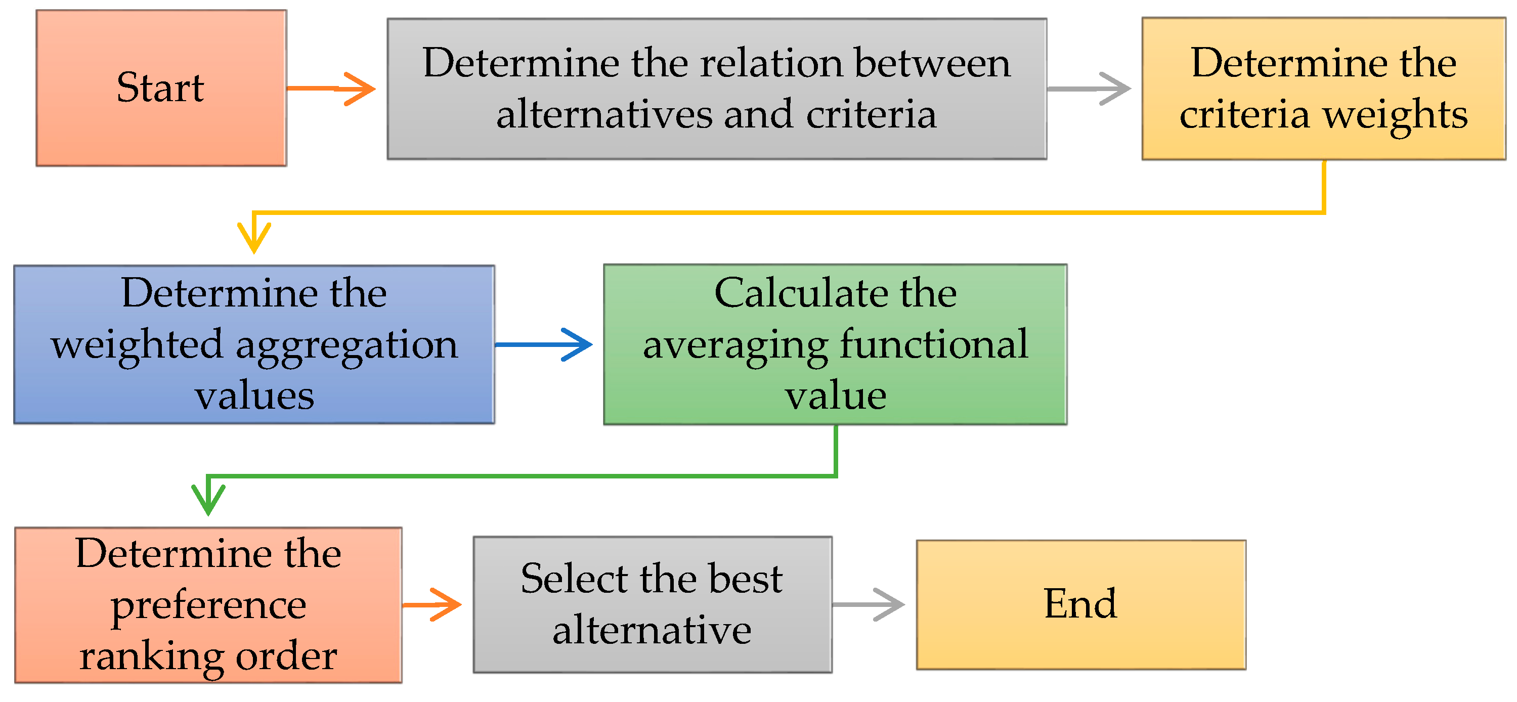
5.2. MCGDM Strategy 2 (Based on NNWHMO)
Strategy 2 is presented (see Figure 2) using the following seven steps:
Step 1. This step is similar to the first step of Strategy 1.
Step 2. Determine the criteria weights.
Using Equation (6), determine the criteria weights from decision matrices (), (t = 1, 2, …, k).
Step 3. Determine the weighted aggregation values ().
Using Equation (4), determine the weighted aggregation values (), (i = 1, 2, …, n) for all decision matrices.
Step 4. Determine the averaging values.
To fuse all the weighted aggregation values (), corresponding to alternatives Ai, we define the averaging function as follows:
Here, wt (t = 1, 2, …, k) is the weight of the decision maker DMt.
Step 5. Determine the ranking order.
Using Equation (1), determine the score values S(zi) (accuracy degrees A(zi), if necessary) (i = 1, 2, …, m) of all alternatives Ai. All the score values are arranged in descending order. The alternative corresponding to the highest score value (accuracy values) reflects the best choice.
Step 6. Select the best alternative from the preference ranking order.
Step 7. End.
6. Simulation Results
We solve a numerical example studied by Zheng et al. [54]. An investment company desires to invest a sum of money in the best investment fund. There are four possible selection options to invest the money. Feasible selection options are namely, A1: Car company (CARC); A2: Food company (FOODC); A3: Computer company (COMC); A4: Arms company (ARMC). Decision-making must be based on the three criteria namely, risk analysis (C1), growth analysis (C2), environmental impact analysis (C3). The four possible selection options/alternatives are to be selected under the criteria by the NN assessments provided by the three decision-makers DM1, DM2, and DM3.
6.1. Solution Using MCGDM Strategy 1
Step 1. Determine the relation between alternatives and criteria.
All assessment values are provided by the following three NN based decision matrices (shown in Equations (10)–(12).
Note 2: Here, , and are the decision matrices for the decision makers DM1, DM2 and DM3 respectively.
Step 2. Determine the weighted aggregation values ().
Using Equation (3), we calculate the aggregation values () as follows:
Step 3. Determine the averaging values.
Using Equation (8), we calculate the averaging values (Considering equal importance of all the decision makers) to fuse all the aggregation values corresponding to the alternative Ai.
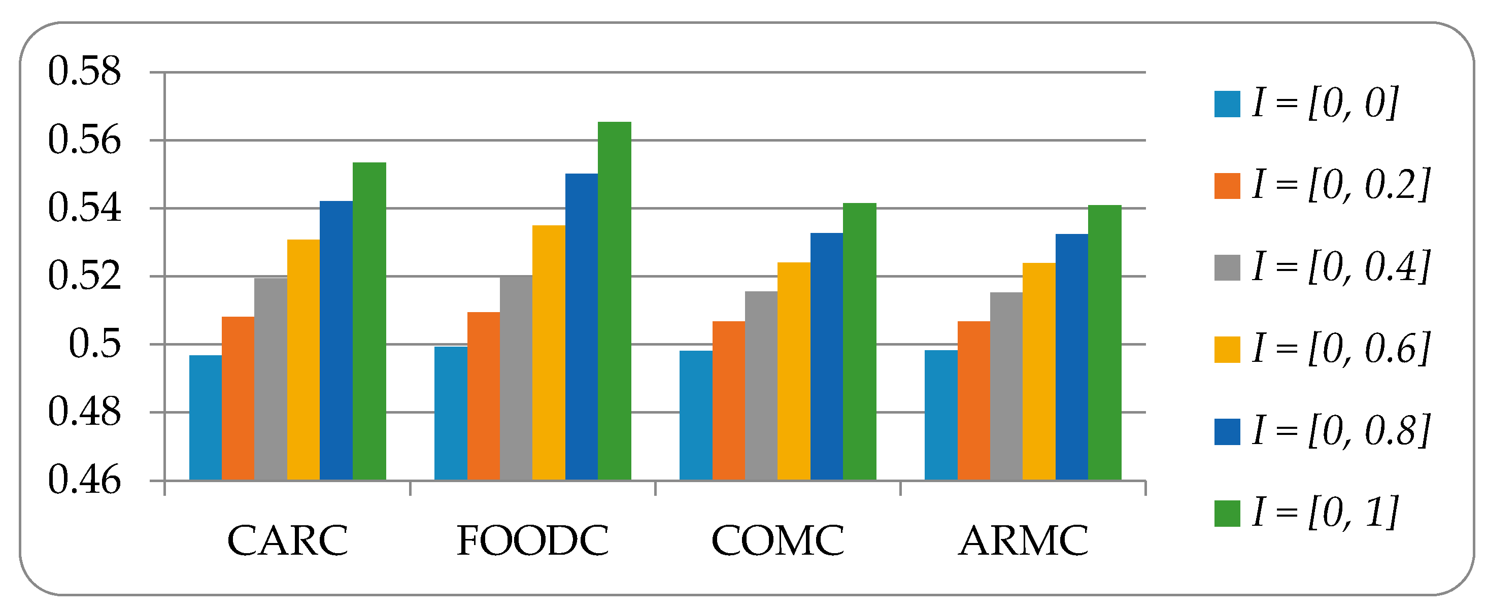
Step 4. Using Equation (1), we calculate the score values Sc(Ai) (i = 1, 2, 3, 4). Sensitivity analysis and ranking order of alternatives are shown in Table 1 for different values of I.
Step 5. Food company (FOODC) is the best alternative for investment.
Step 6. End.
6.2. Solution Using MCGDM Strategy 2
Step 1. Determine the relation between alternatives and criteria.
This step is similar to the first step of strategy 1.
Step 2. Determine the criteria weights.
Using Equations (5) and (6), criteria weights are calculated as follows:
[w1 = 0.3265, w2 = 0.3430, w3 = 0.3305] for DM1,
[w1 = 0.3332, w2 = 0.3334, w3 = 0.3334] for DM2,
[w1 = 0.3333, w2 = 0.3335, w3 = 0.3332] for DM3.
Step 3. Determine the weighted aggregation values ().
Using Equation (4), we calculate the aggregation values () as follows:
Step 4. Determine the averaging values.
Using Equation (9), we calculate the averaging (Considering equal importance of all the decision makers to fuse all the aggregation values corresponding to the alternative Ai.
Step 5. Determine the ranking order.
Using Equation (1), we calculate the score values Sc(Ai) (i = 1, 2, 3, 4). Since scores values are different, accuracy values are not required. Sensitivity analysis and ranking order of alternatives are shown in Table 2 for different values of I.
Step 6. Food company (FOODC) is the best alternative for investment.
Step 7. End.
7. Comparison Analysis and Contributions of the Proposed Approach
7.1. Comparison Analysis
In this subsection, a comparison analysis is conducted between the proposed MCGDM strategies and the other existing strategies in the literature in NN environment. Table 1 reflects that A2 is the best alternative for I = 0 and i.e., for all cases considered. Table 2 reflects that A2 is the best alternative for any values of I. Ranking order differs for different values of I.
The ranking results obtained from the existing strategies [52,53,54] are furnished in Table 3. The ranking orders of Ye [52] and Zheng et al. [54] are similar for all values of I considered. When I lies in [0, 0], [0, 0.2], [0, 0.4], A2 is the best alternative for [52,53,54] and the proposed strategies. When I lies in [0, 0.6], [0, 0.8], [0, 1], A4 is the best alternative for [52,54], whereas A2 is the best alternative for [53], and the proposed strategies.
In strategy [52], deneutrosophication process is analyzed. It does not recognize the importance of the aggregation information. MCGDM due to Liu and Liu [53] is based on NN generalized weighted power averaging operator. This strategy cannot deal the situation when larger value other than arithmetic mean, geometric mean, and harmonic mean is necessary for experimental purpose.
The strategy proposed by Zheng et al. [54] cannot be used when few observations contribute disproportionate amount to the arithmetic mean. The proposed two MCGDM strategies are free from these shortcomings.
7.2. Contributions of the Proposed Approach
- NNHMO and NNWHMO in NN environment are firstly defined in the literature. We have also proved their basic properties.
- We have proposed score and accuracy functions of NN numbers for ranking. If two score values are same, then accuracy function can be used for ranking purpose.
- The proposed two strategies can also be used when observations/experiments contribute is disproportionate amount to the arithmetic mean. The harmonic mean is used when sample values contain fractions and/or extreme values (either too small or too big).
- To calculate unknown weights structure of criteria in NN environment, we have proposed cosine function.
- Steps and calculations of the proposed strategies are easy to use.
- We have solved a numerical example to show the feasibility, applicability, and effectiveness of the proposed two strategies.
8. Conclusions
In the study, we have proposed NNHMO and NNWHMO. We have developed two strategies of ranking NNs based on proposed score and accuracy functions. We have proposed a cosine function to determine unknown weights of the criteria in a NN environment. We have developed two novel MCGDM strategies based on the proposed aggregation operators. We have solved a hypothetical case study and compared the obtained results with other existing strategies to demonstrate the effectiveness of the proposed MCGDM strategies. Sensitivity analysis for different values of I is also conducted to show the influence of I in preference ranking of the alternatives. The proposed MCGDM strategies can be applied in supply selection, pattern recognition, cluster analysis, medical diagnosis, etc.
Acknowledgments
The authors are very grateful to the anonymous reviewers for their insightful and constructive comments and suggestions that have led to an improved version of this paper.
Author Contributions
Kalyan Mondal and Surapati Pramanik conceived and designed the experiments; Kalyan Mondal, and Surapati Pramanik performed the experiments; Surapati Pramanik, Bibhas C. Giri, and Florentine Smarandache analyzed the data; Kalyan Mondal, Surapati Pramanik, Bibhas C. Giri, and Florentine Smarandache contributed to the analysis tools; and Kalyan Mondal and Surapati Pramanik wrote the paper.
Conflicts of Interest
The authors declare no conflict of interest.
References
- Hwang, L.; Lin, M.J. Group Decision Making under Multiple Criteria: Methods and Applications; Springer: Heidelberg, Germany, 1987. [Google Scholar]
- Hwang, C.; Yoon, K. Multiple Attribute Decision Making, Methods and Applications; Springer: New York, NY, USA, 1981; Volume 186. [Google Scholar]
- Chen, S.J.; Hwang, C.L. Fuzzy Multiple Attribute Decision-Making, Methods and Applications; Lecture Notes in Economics and Mathematical Systems; Springer: Berlin/Heidelberg, Germany, 1992; Volume 375. [Google Scholar]
- Chang, T.H.; Wang, T.C. Using the fuzzy multi-criteria decision making approach for measuring the possibility of successful knowledge management. Inf. Sci. 2009, 179, 355–370. [Google Scholar] [CrossRef]
- Krohling, R.A.; De Souza, T.T.M. Combining prospect theory and fuzzy numbers to multi-criteria decision making. Exp. Syst. Appl. 2012, 39, 11487–11493. [Google Scholar] [CrossRef]
- Chen, C.T. Extension of the TOPSIS for group decision-making under fuzzy environment. Fuzzy Sets Syst. 2000, 114, 1–9. [Google Scholar] [CrossRef]
- Zhang, G.; Lu, J. An integrated group decision-making method dealing with fuzzy preferences for alternatives and individual judgments for selection criteria. Group Decis. Negot. 2003, 12, 501–515. [Google Scholar] [CrossRef]
- Krohling, R.A.; Campanharo, V.C. Fuzzy TOPSIS for group decision making: A case study for accidents with oil spill in the sea. Exp. Syst. Appl. 2011, 38, 4190–4197. [Google Scholar] [CrossRef]
- Xia, M.; Xu, Z. A novel method for fuzzy multi-criteria decision making. Int. J. Inf. Technol. Decis. Mak. 2014, 13, 497–519. [Google Scholar] [CrossRef]
- Mehlawat, M.K.; Guptal, P. A new fuzzy group multi-criteria decision making method with an application to the critical path selection. Int. J. Adv. Manuf. Technol. 2015. [Google Scholar] [CrossRef]
- Lin, L.; Yuan, X.H.; Xia, Z.Q. Multicriteria fuzzy decision-making based on intuitionistic fuzzy sets. J. Comput. Syst. Sci. 2007, 73, 84–88. [Google Scholar] [CrossRef]
- Liu, H.W.; Wang, G.J. Multi-criteria decision-making methods based on intuitionistic fuzzy sets. Eur. J. Oper. Res. 2007, 179, 220–233. [Google Scholar] [CrossRef]
- Pramanik, S.; Mondal, K. Weighted fuzzy similarity measure based on tangent function and its application to medical diagnosis. Int. J. Innov. Res. Sci. Eng. Technol. 2015, 4, 158–164. [Google Scholar]
- Pramanik, S.; Mukhopadhyaya, D. Grey relational analysis based intuitionistic fuzzy multi-criteria group decision-making approach for teacher selection in higher education. Int. J. Comput. Appl. 2011, 34, 21–29. [Google Scholar] [CrossRef]
- Mondal, K.; Pramanik, S. Intuitionistic fuzzy multi criteria group decision making approach to quality-brick selection problem. J. Appl. Quant. Methods 2014, 9, 35–50. [Google Scholar]
- Dey, P.P.; Pramanik, S.; Giri, B.C. Multi-criteria group decision making in intuitionistic fuzzy environment based on grey relational analysis for weaver selection in Khadi institution. J. Appl. Quant. Methods 2015, 10, 1–14. [Google Scholar]
- Ye, J. Multicriteria fuzzy decision-making method based on the intuitionistic fuzzy cross-entropy. In Proceedings of the International Conference on Intelligent Human-Machine Systems and Cybernetics, Hangzhou, China, 26–27 August 2009. [Google Scholar]
- Chen, S.M.; Chang, C.H. A novel similarity measure between Atanassov’s intuitionistic fuzzy sets based on transformation techniques with applications to pattern recognition. Inf. Sci. 2015, 291, 96–114. [Google Scholar] [CrossRef]
- Chen, S.M.; Cheng, S.H.; Chiou, C.H. Fuzzy multi-attribute group decision making based on intuitionistic fuzzy sets and evidential reasoning methodology. Inf. Fusion 2016, 27, 215–227. [Google Scholar] [CrossRef]
- Wang, J.Q.; Han, Z.Q.; Zhang, H.Y. Multi-criteria group decision making method based on intuitionistic interval fuzzy information. Group Decis. Negot. 2014, 23, 715–733. [Google Scholar] [CrossRef]
- Yue, Z.L. TOPSIS-based group decision-making methodology in intuitionistic fuzzy setting. Inf. Sci. 2014, 277, 141–153. [Google Scholar] [CrossRef]
- He, X.; Liu, W.F. An intuitionistic fuzzy multi-attribute decision-making method with preference on alternatives. Oper. Res Manag. Sci. 2013, 22, 36–40. [Google Scholar]
- Mondal, K.; Pramanik, S. Intuitionistic fuzzy similarity measure based on tangent function and its application to multi-attribute decision making. Glob. J. Adv. Res. 2015, 2, 464–471. [Google Scholar]
- Peng, H.G.; Wang, J.Q.; Cheng, P.F. A linguistic intuitionistic multi-criteria decision-making method based on the Frank Heronian mean operator and its application in evaluating coal mine safety. Int. J. Mach. Learn. Cybern. 2016. [Google Scholar] [CrossRef]
- Liang, R.X.; Wang, J.Q.; Zhang, H.Y. A multi-criteria decision-making method based on single-valued trapezoidal neutrosophic preference relations with complete weight information. Neural Comput. Appl. 2017. [Google Scholar] [CrossRef]
- Wang, J.Q.; Yang, Y.; Li, L. Multi-criteria decision-making method based on single-valued neutrosophic linguistic Maclaurin symmetric mean operators. Neural Comput. Appl. 2016. [Google Scholar] [CrossRef]
- Kharal, A. A neutrosophic multi-criteria decision making method. New Math. Nat. Comput. 2014, 10, 143–162. [Google Scholar] [CrossRef]
- Ye, J. Multiple attribute group decision-making method with completely unknown weights based on similarity measures under single valued neutrosophic environment. J. Intell. Fuzzy Syst. 2014, 27, 2927–2935. [Google Scholar]
- Mondal, K.; Pramanik, S. Multi-criteria group decision making approach for teacher recruitment in higher education under simplified neutrosophic environment. Neutrosophic Sets Syst. 2014, 6, 28–34. [Google Scholar]
- Biswas, P.; Pramanik, S.; Giri, B.C. A new methodology for neutrosophic multi-attribute decision-making with unknown weight information. Neutrosophic Sets Syst. 2014, 3, 44–54. [Google Scholar]
- Biswas, P.; Pramanik, S.; Giri, B.C. Cosine similarity measure based multi-attribute decision-making with trapezoidal fuzzy neutrosophic numbers. Neutrosophic Sets Syst. 2014, 8, 46–56. [Google Scholar]
- Mondal, K.; Pramanik, S. Neutrosophic decision making model for clay-brick selection in construction field based on grey relational analysis. Neutrosophic Sets Syst. 2015, 9, 64–71. [Google Scholar]
- Mondal, K.; Pramanik, S. Neutrosophic tangent similarity measure and its application to multiple attribute decision making. Neutrosophic Sets Syst. 2015, 9, 85–92. [Google Scholar]
- Pramanik, S.; Biswas, P.; Giri, B.C. Hybrid vector similarity measures and their applications to multi-attribute decision making under neutrosophic environment. Neural Comput. Appl. 2015. [Google Scholar] [CrossRef]
- Sahin, R.; Küçük, A. Subsethood measure for single valued neutrosophic sets. J. Intell. Fuzzy Syst. 2015, 29, 525–530. [Google Scholar] [CrossRef]
- Mondal, K.; Pramanik, S. Neutrosophic decision making model of school choice. Neutrosophic Sets Syst. 2015, 7, 62–68. [Google Scholar]
- Ye, J. An extended TOPSIS method for multiple attribute group decision making based on single valued neutrosophic linguistic numbers. J. Intell. Fuzzy Syst. 2015, 28, 247–255. [Google Scholar]
- Biswas, P.; Pramanik, S.; Giri, B.C. TOPSIS method for multi-attribute group decision-making under single-valued neutrosophic environment. Neural Comput. Appl. 2016, 27, 727–737. [Google Scholar] [CrossRef]
- Biswas, P.; Pramanik, S.; Giri, B.C. Value and ambiguity index based ranking method of single-valued trapezoidal neutrosophic numbers and its application to multi-attribute decision making. Neutrosophic Sets Syst. 2016, 12, 127–138. [Google Scholar]
- Biswas, P.; Pramanik, S.; Giri, B.C. Aggregation of triangular fuzzy neutrosophic set information and its application to multi-attribute decision making. Neutrosophic Sets Syst. 2016, 12, 20–40. [Google Scholar]
- Smarandache, F.; Pramanik, S. (Eds.) New Trends in Neutrosophic Theory and Applications; Pons Editions: Brussels, Belgium, 2016; pp. 15–161. ISBN 978-1-59973-498-9. [Google Scholar]
- Sahin, R.; Liu, P. Maximizing deviation method for neutrosophic multiple attribute decision making with incomplete weight information. Neural Comput. Appl. 2016, 27, 2017–2029. [Google Scholar] [CrossRef]
- Pramanik, S.; Dalapati, S.; Alam, S.; Smarandache, S.; Roy, T.K. NS-cross entropy based MAGDM under single valued neutrosophic set environment. Information 2018, 9, 37. [Google Scholar] [CrossRef]
- Sahin, R.; Liu, P. Possibility-induced simplified neutrosophic aggregation operators and their application to multi-criteria group decision-making. J. Exp. Theor. Artif. Intell. 2017, 29, 769–785. [Google Scholar] [CrossRef]
- Biswas, P.; Pramanik, S.; Giri, B.C. Multi-attribute group decision making based on expected value of neutrosophic trapezoidal numbers. New Math. Nat. Comput. 2017, in press. [Google Scholar]
- Smarandache, F. Introduction to Neutrosophic Measure, Neutrosophic Integral, and Neutrosophic, Probability; Sitech & Education Publisher: Craiova, Romania, 2013. [Google Scholar]
- Smarandache, F. Introduction to Neutrosophic Statistics; Sitech & Education Publishing: Columbus, OH, USA, 2014. [Google Scholar]
- Xu, Z. Fuzzy harmonic mean operators. Int. J. Intell. Syst. 2009, 24, 152–172. [Google Scholar] [CrossRef]
- Park, J.H.; Gwak, M.G.; Kwun, Y.C. Uncertain linguistic harmonic mean operators and their applications to multiple attribute group decision making. Computing 2011, 93, 47–64. [Google Scholar] [CrossRef]
- Wei, G.W. FIOWHM operator and its application to multiple attribute group decision making. Expert Syst. Appl. 2011, 38, 2984–2989. [Google Scholar] [CrossRef]
- Ye, J. Simplified neutrosophic harmonic averaging projection-based strategy for multiple attribute decision-making problems. Int. J. Mach. Learn. Cybern. 2017, 8, 981–987. [Google Scholar] [CrossRef]
- Ye, J. Multiple attribute group decision making method under neutrosophic number environment. J. Intell. Syst. 2016, 25, 377–386. [Google Scholar] [CrossRef]
- Liu, P.; Liu, X. The neutrosophic number generalized weighted power averaging operator and its application in multiple attribute group decision making. Int. J. Mach. Learn. Cybern. 2016, 1–12. [Google Scholar] [CrossRef]
- Zheng, E.; Teng, F.; Liu, P. Multiple attribute group decision-making strategy based on neutrosophic number generalized hybrid weighted averaging operator. Neural Comput. Appl. 2017, 28, 2063–2074. [Google Scholar] [CrossRef]
- Pramanik, S.; Roy, R.; Roy, T.K. Teacher selection strategy based on bidirectional projection measure in neutrosophic number environment. In Neutrosophic Operational Research; Smarandache, F., Abdel-Basset, M., El-Henawy, I., Eds.; Pons Publishing House: Bruxelles, Belgium, 2017; Volume 2, ISBN 978-1-59973-537-5. [Google Scholar]
- Majumdar, P.; Samanta, S.K. On similarity and entropy of neutrosophic sets. J. Intell. Fuzzy Syst. 2014, 26, 1245–1252. [Google Scholar]
- Biswas, P.; Pramanik, S.; Giri, B.C. Entropy based grey relational analysis strategy for multi-attribute decision-making under single valued neutrosophic assessments. Neutrosophic Sets. Syst. 2014, 2, 102–110. [Google Scholar]
Figure 1.
Steps of MCGDM Strategy 1 based on NNHMO.
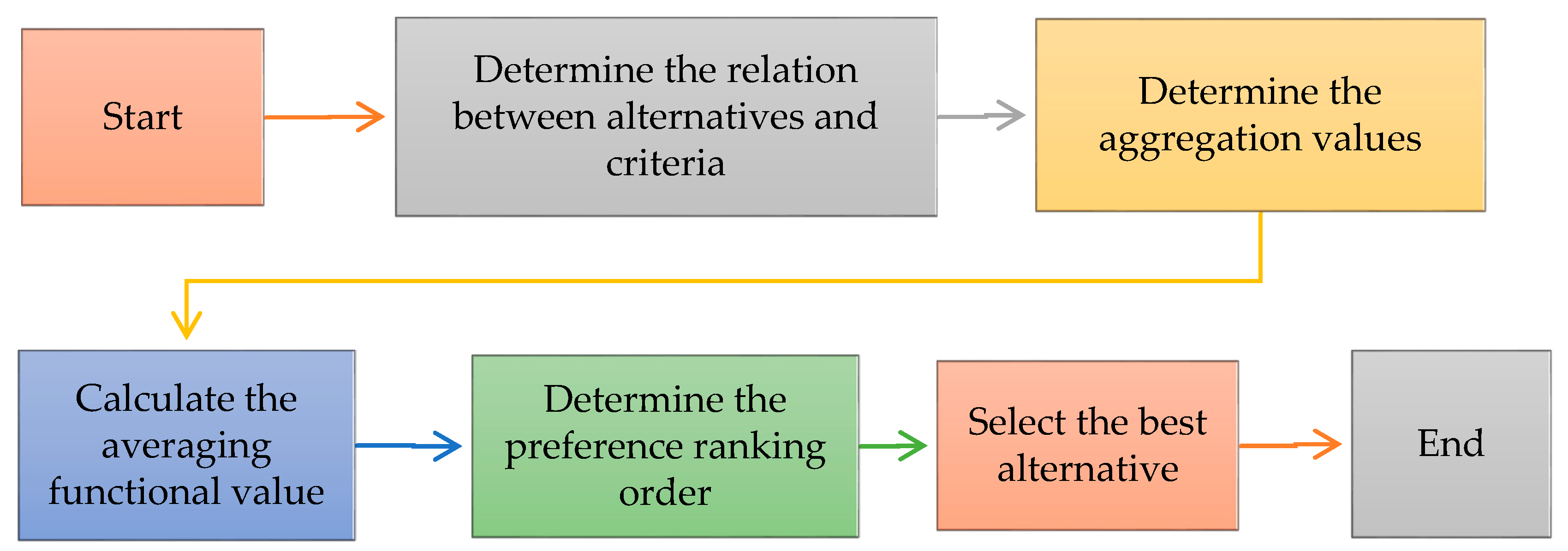
Figure 2.
Steps of MCGDM strategy based on NNWHMO.

Figure 3.
Ranking order with variation of “I” based on strategy 1.
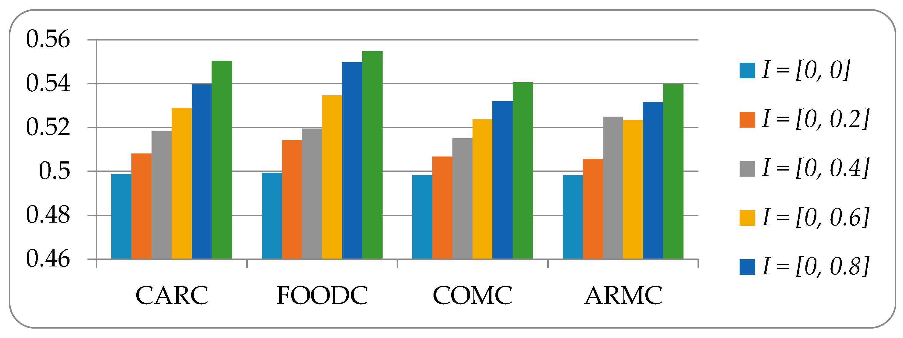
Figure 4.
Ranking order with variation of “I” on NNs for Strategy 2.


Table 1.
Sensitivity analysis and ranking order with variation of “I” on NNs for strategy 1.
| I | Sc(Ai) | Ranking Order |
|---|---|---|
| I = [0, 0] | S(A1) = 0.4988, S(A2) = 0.4993, S(A3) = 0.4982, S(A4) = 0.4983 | A2 A1 A4 A3 |
| I [0, 0.2] | S(A1) = 0.5081, S(A2) = 0.5144, S(A3) = 0.5067, S(A4) = 0.5056 | A2 A1 A3 A4 |
| I [0, 0.4] | S(A1) = 0.5182, S(A2) = 0.5195, S(A3) = 0.5151, S(A4) = 0.5249 | A2 A1 A4 A3 |
| I [0, 0.6] | S(A1) = 0.5289, S(A2) = 0.5346, S(A3) = 0.5236, S(A4) = 0.5233 | A2 A1 A3 A4 |
| I [0, 0.8] | S(A1) = 0.5396, S(A2) = 0.5497, S(A3) = 0.5320, S(A4) = 0.5316 | A2 A1 A3 A4 |
| I [0, 1] | S(A1) = 0.5503, S(A2) = 0.5547, S(A3) = 0.5405, S(A4) = 0.5399 | A2 A1 A3 A4 |
Table 2.
Sensitivity analysis and ranking order with variation of “I” on NNs for strategy 2.
| I | Sc(Ai) | Ranking Order |
|---|---|---|
| I = 0 | S(A1) = 0.4968, S(A2) = 0.4993, S(A3) = 0.4981, S(A4) = 0.4982 | A2 A4 A3 A1 |
| I [0, 0.2] | S(A1) = 0.5081, S(A2) = 0.5095, S(A3) = 0.5068, S(A4) = 0.5067 | A2 A1 A4 A3 |
| I [0, 0.4] | S(A1) = 0.5195, S(A2) = 0.5198, S(A3) = 0.5155, S(A4) = 0.5153 | A2 A1 A3 A4 |
| I [0, 0.6] | S(A1) = 0.5308, S(A2) = 0.5350, S(A3) = 0.5241, S(A4) = 0.5239 | A2 A1 A3 A4 |
| I [0, 0.8] | S(A1) = 0.5421, S(A2) = 0.5502, S(A3) = 0.5328, S(A4) = 0.5324 | A2 A1 A3 A4 |
| I [0, 1] | S(A1) = 0.5535, S(A2) = 0.5654, S(A3) = 0.5415, S(A4) = 0.5410 | A2 A1 A3 A4 |
Table 3.
Comparison of ranking preference order with variation of “I” on NNs for different strategies.
Table 3.
Comparison of ranking preference order with variation of “I” on NNs for different strategies.
| I | Ye [52] | Zheng et al. [54] | Liu and Liu [53] | Proposed Strategy 1 | Proposed Strategy 2 |
|---|---|---|---|---|---|
| [0, 0] | A2 A4 A3 A1 | A2 A4 A3 A1 | A2 A4 A1 A3 | A2 A1 A4 A3 | A2 A4 A3 A1 |
| [0, 0.2] | A2 A4 A3 A1 | A2 A4 A3 A1 | A2 A3 A1 A4 | A2 A1 A3 A4 | A2 A1 A4 A3 |
| [0, 0.4] | A2 A4 A3 A1 | A2 A4 A3 A1 | A2 A3 A4 A1 | A2 A1 A4 A3 | A2 A1 A3 A4 |
| [0, 0.6] | A4 A2 A3 A1 | A4 A2 A3 A1 | A2 A3 A4 A1 | A2 A1 A3 A4 | A2 A1 A3 A4 |
| [0, 0.8] | A4 A2 A3 A1 | A4 A2 A3 A1 | A2 A3 A4 A1 | A2 A1 A3 A4 | A2 A1 A3 A4 |
| [0, 1] | A4 A2 A3 A1 | A4 A2 A3 A1 | A2 A4 A3 A1 | A2 A1 A3 A4 | A2 A1 A3 A4 |
© 2018 by the authors. Licensee MDPI, Basel, Switzerland. This article is an open access article distributed under the terms and conditions of the Creative Commons Attribution (CC BY) license (http://creativecommons.org/licenses/by/4.0/).
Share and Cite
MDPI and ACS Style
Mondal, K.; Pramanik, S.; Giri, B.C.; Smarandache, F. NN-Harmonic Mean Aggregation Operators-Based MCGDM Strategy in a Neutrosophic Number Environment. Axioms 2018, 7, 12. https://doi.org/10.3390/axioms7010012
AMA Style
Mondal K, Pramanik S, Giri BC, Smarandache F. NN-Harmonic Mean Aggregation Operators-Based MCGDM Strategy in a Neutrosophic Number Environment. Axioms. 2018; 7(1):12. https://doi.org/10.3390/axioms7010012
Chicago/Turabian StyleMondal, Kalyan, Surapati Pramanik, Bibhas C. Giri, and Florentin Smarandache. 2018. "NN-Harmonic Mean Aggregation Operators-Based MCGDM Strategy in a Neutrosophic Number Environment" Axioms 7, no. 1: 12. https://doi.org/10.3390/axioms7010012
Note that from the first issue of 2016, this journal uses article numbers instead of page numbers. See further details here.