Multi-Attribute Decision-Making Method Based on Neutrosophic Soft Rough Information


1
Department of Mathematics, University of the Punjab, New Campus, Lahore 54590, Pakistan
2
Mathematics & Science Department, University of New Mexico, 705 Gurley Ave., Gallup, NM 87301, USA
*
Author to whom correspondence should be addressed.
Axioms 2018, 7(1), 19; https://doi.org/10.3390/axioms7010019
Submission received: 17 February 2018
/
Revised: 14 March 2018
/
Accepted: 19 March 2018
/
Published: 20 March 2018
(This article belongs to the Special Issue Neutrosophic Multi-Criteria Decision Making)
Abstract
:Soft sets (SSs), neutrosophic sets (NSs), and rough sets (RSs) are different mathematical models for handling uncertainties, but they are mutually related. In this research paper, we introduce the notions of soft rough neutrosophic sets (SRNSs) and neutrosophic soft rough sets (NSRSs) as hybrid models for soft computing. We describe a mathematical approach to handle decision-making problems in view of NSRSs. We also present an efficient algorithm of our proposed hybrid model to solve decision-making problems.
MSC:
03E72; 68R10; 68R051. Introduction
Smarandache [1] initiated the concept of neutrosophic set (NS). Smarandache’s NS is characterized by three parts: truth, indeterminacy, and falsity. Truth, indeterminacy and falsity membership values behave independently and deal with the problems of having uncertain, indeterminant and imprecise data. Wang et al. [2] gave a new concept of single valued neutrosophic set (SVNS) and defined the set of theoretic operators in an instance of NS called SVNS. Ye [3,4,5] studied the correlation coefficient and improved correlation coefficient of NSs, and also determined that, in NSs, the cosine similarity measure is a special case of the correlation coefficient. Peng et al. [6] discussed the operations of simplified neutrosophic numbers and introduced an outranking idea of simplified neutrosophic numbers.
Molodtsov [7] introduced the notion of soft set as a novel mathematical approach for handling uncertainties. Molodtsov’s soft sets give us new technique for dealing with uncertainty from the viewpoint of parameters. Maji et al. [8,9,10] introduced neutrosophic soft sets (NSSs), intuitionistic fuzzy soft sets (IFSSs) and fuzzy soft sets (FSSs). Babitha and Sunil gave the idea of soft set relations [11]. In [12], Sahin and Kucuk presented NSS in the form of neutrosophic relation.
Rough set theory was initiated by Pawlak [13] in 1982. Rough set theory is used to study the intelligence systems containing incomplete, uncertain or inexact information. The lower and upper approximation operators of RSs are used for managing hidden information in a system. Therefore, many hybrid models have been built such as soft rough sets (SRSs), rough fuzzy sets (RFSs), fuzzy rough sets (FRSs), soft fuzzy rough sets (SFRSs), soft rough fuzzy sets (SRFSs), intuitionistic fuzzy soft rough sets (IFSRS), neutrosophic rough sets (NRSs), and rough neutrosophic sets (RNSs) for handling uncertainty and incomplete information effectively. Soft set theory and RS theory are two different mathematical tools to deal with uncertainty. Evidently, there is no direct relationship between these two mathematical tools, but efforts have been made to define some kind of relation [14,15]. Feng et al. [15] took a significant step to introduce parametrization tools in RSs. They introduced SRSs, in which parameterized subsets of universal sets are elementary building blocks for approximation operators of a subset. Shabir et al. [16] introduced another approach to study roughness through SSs, and this approach is known as modified SRSs (MSR-sets). In MSR-sets, some results proved to be valid that failed to hold in SRSs. Feng et al. [17] introduced a modification of Pawlak approximation space known as soft approximation space (SAS) in which SAS SRSs were proposed. Moreover, they introduced soft rough fuzzy approximation operators in SAS and initiated a idea of SRFSs, which is an extension of RFSs introduced by Dubois and Prade [18] . Meng et al. [19] provide further discussion of the combination of SSs, RSs and FSs. In various decision-making problems, RSs have been used. The existing results of RSs and other extended RSs such as RFSs, generalized RFSs, SFRSs and IFRSs based decision-making models have their advantages and limitations [20,21]. In a different way, RS approximations have been constructed into the IF environment and are known as IFRSs, RIFSs and generalized IFRSs [22,23,24]. Zhang et al. [25,26] presented the notions of SRSs, SRIFSs, and IFSRSs, its application in decision-making, and also introduced generalized IFSRSs. Broumi et al. [27,28] developed a hybrid structure by combining RSs and NSs, called RNSs. They also presented interval valued neutrosophic soft rough sets by combining interval valued neutrosophic soft sets and RSs. Yang et al. [29] proposed single valued neutrosophic rough sets (SVNRSs) by combining SVNSs and RSs, and established an algorithm for decision-making problems based on SVNRSs in two universes. For some papers related to NSs and multi-criteria decision-making (MCDM), the readers are referred to [30,31,32,33,34,35,36,37,38]. The notion of SRNSs is a extension of SRSs, SRIFSs, IFSRSs, introduced by Zhang et al. motivated by the idea of single valued neutrosophic rough sets (SVNRSs) introduced, we extend the single valued neutrosophic rough sets’ lower and upper approximations to the case of a neutrosophic soft rough set. The concept of a neutrosophic soft rough set is introduced by coupling both the neutrosophic soft sets and rough sets. In this research paper, we introduce the notions of SRNSs and NSRSs as hybrid models for soft computing. Approximation operators of SRNSs and NSRSs are described and their relevant properties are investigated in detail. We describe a mathematical approach to handle decision-making problems in view of NSRSs. We also present an efficient algorithm of our proposed hybrid model to solve decision-making problems.
2. Construction of Soft Rough Neutrosophic Sets
In this section, we introduce the notions of SRNSs by combining soft sets with RNSs and soft rough neutrosophic relations (SRNRs). Soft rough neutrosophic sets consist of two basic components, namely neutrosophic sets and soft relations, which are the mathematical basis of SRNSs. The basic idea of soft rough neutrosophic sets is based on the approximation of sets by a couple of sets known as the lower soft rough neutrosophic approximation and the upper soft rough neutrosophic approximation of a set. Here, the lower and upper approximation operators are based on an arbitrary soft relation. The concept of soft rough neutrosophic sets is an extension of the crisp set, rough set for the study of intelligent systems characterized by inexact, uncertain or insufficient information. It is a useful tool for dealing with uncertainty or imprecision information. The concept of neutrosophic soft sets is powerful logic to handle indeterminate and inconsistent situations, and the theory of rough neutrosophic sets is also powerful mathematical logic to handle incompleteness. We introduce the notions of soft rough neutrosophic sets (SRNSs) and neutrosophic soft rough sets (NSRSs) as hybrid models for soft computing. The rating of all alternatives is expressed with the upper soft rough neutrosophic approximation and lower soft rough neutrosophic approximation operator and the pair of neutrosophic sets that are characterized by truth-membership degree, indeterminacy-membership degree, and falsity-membership degree from the view point of parameters.
Definition 1.
Let Y be an initial universal set and M a universal set of parameters. For an arbitrary soft relation P over , let be a set-valued function defined as
Let be an SAS. For any NS , where is a neutrosophic power set of parameter set the lower soft rough neutrosophic approximation (LSRNA) and the upper soft rough neutrosophic approximation (USRNA) operators of C w.r.t denoted by and are, respectively, defined as follows:
where
It is observed that and are two NSs on Y, are referred to as the LSRNA and the USRNA operators, respectively. The pair is called SRNS of C w.r.t .
Remark 1.
Let be an SAS. If and , where and are intuitionistic fuzzy power set and crisp power set of M, respectively. Then, the above SRNA operators and degenerate to SRIFA and SRA operators, respectively. Hence, SRNA operators are an extension of SRIFA and SRA operators.
Example 1.
Suppose that is the set of five careers under observation, and Mr. X wants to select best suitable career. Let be a set of decision parameters. The parameters and stand for “aptitude”, “work value”, “skill” and “recent advancement”, respectively. Mr. X describes the “most suitable career” by defining a soft relation P from Y to M, which is a crisp soft set as shown in Table 1.
is a set valued function, and we have and Mr. X gives most the favorable parameter object C, which is an NS defined as follows:
From the Definition 1, we have
Similarly,
Thus, we obtain
Hence, is an SRNS of C.
Theorem 1.
Let be an SAS. Then, the LSRNA and the USRNA operators and satisfy the following properties for all :
- (i)
- (ii)
- (iii)
- (iv)
- (v)
- (vi)
- (vii)
- (viii)
where is the complement of C.
Proof.
- (i)
- By definition of SRNS, we havewhereHence, .
- (ii)
- (iii)
- It can be easily proved by Definition 1.
- (iv)
Similarly, we can prove that
Thus, .
The properties (v)–(viii) of the USRNA can be easily proved similarly. ☐
Example 2.
Considering Example 1, we have
Clearly, . Hence, properties of the LSRNA operator hold, and we can easily verify the properties of the USRNA operator.
The conventional soft set is a mapping from a parameter to the subset of universe and let be a crisp soft set. In [11], Babitha and Sunil introduced the concept of soft set relation. Now, we present the constructive definition of SRNR by using a soft relation R from to , where Y is a universal set and M is a set of parameter.
Definition 2.
A SRNR on Y is a SRNS, is a soft relation on Y defined by
Let be a set-valued function by
For any the USRNA and the LSRNA operators of D w.r.t defined as follows:
where
The pair is called SRNR and are called the LSRNA and the USRNA operators, respectively.
Remark 2.
For an NS D on and an NS C on M,
According to the definition of SRNR, we get
Similarly, for the LSRNA operator ,
Example 3.
Let be a universal set and be a set of parameters. A soft set on Y can be defined in tabular form (see Table 2) as follows:
Let and . Then, a soft relation R on E (from L to E) can be defined in tabular form (see Table 3) as follows:
Now, we can define set-valued function such that
- Let be an NS on M, then
- Let be an NS on then
Hence, is SRNR.
3. Construction of Neutrosophic Soft Rough Sets
In this section, we will introduce the notions of NSRSs, neutrosophic soft rough relations (NSRRs).
Definition 3.
Let Y be an initial universal set and M a universal set of parameters. For an arbitrary neutrosophic soft relation from Y to M, is called neutrosophic soft approximation space (NSAS). For any NS we define the upper neutrosophic soft approximation (UNSA) and the lower neutrosophic soft approximation (LNSA) operators of C with respect to denoted by and respectively as follows:
where
The pair is called NSRS of C w.r.t and are referred to as the LNSRA and the UNSRA operators, respectively.
Remark 3.
A neutrosophic soft relation over is actually a neutrosophic soft set on Y. The NSRA operators are defined over two distinct universes Y and M. As we know, universal set Y and parameter set M are two different universes of discourse but have solid relations. These universes can not be considered as identical universes; therefore, the reflexive, symmetric and transitive properties of neutrosophic soft relations from Y to M do not exist.
Let be a neutrosophic soft relation from Y to M, if, for each , there exists such that . Then, is referred to as a serial neutrosophic soft relation from Y to parameter set M.
Example 4.
Suppose that is the set of careers under consideration, and Mr. X wants to select the most suitable career. is a set of decision parameters. Mr. X describes the “most suitable career” by defining a neutrosophic soft set on Y that is a neutrosophic relation from Y to M as shown in Table 4.
Now, Mr. X gives the most favorable decision object C, which is an NS on M defined as follows: . By Definition 3, we have
Similarly,
Thus, we obtain
Hence, is an NSRS of C.
Theorem 2.
Let be an NSAS. Then, the UNSRA and the LNSRA operators and satisfy the following properties for all :
- (i)
- (ii)
- (iii)
- (iv)
- (v)
- (vi)
- (vii)
- (viii)
Proof.
- (i)
- (ii)
- Now, consider
- (iii)
- It can be easily proven by Definition 3.
- (iv)
- (vii)
The properties (v)–(vii) of the UNSRA operator can be easily proved similarly. ☐
Theorem 3.
Let be an NSAS. The UNSRA and the LNSRA operators and satisfy the following properties for all :
- (i)
- ,
- (ii)
Proof.
- (i)
- By Definition 3 and definition of difference of two NSs, for all
- (ii)
- By Definition 3 and definition of difference of two NSs, for all
☐
Theorem 4.
Let be an NSAS. If is serial, then the UNSA and the LNSA operators and satisfy the following properties for all :
- (i)
- (ii)
Proof.
- (i)
- Since ∅ is a null NS on M,Now,Since is full NS on , for all , and this implies Thus,
- (ii)
- Since is an NSAS and is a serial neutrosophic soft relation, then, for each , there exists , such that and . The UNSRA and LNSRA operators , and of an NS C can be defined as:Clearly, for all Thus, .☐
The conventional NSS is a mapping from a parameter to the neutrosophic subset of universe and let be NSS. Now, we present the constructive definition of neutrosophic soft rough relation by using a neutrosophic soft relation from to , where Y is a universal set and M is a set of parameters.
Definition 4.
A neutrosophic soft rough relation on Y is an NSRS, is a neutrosophic soft relation on Y defined by
such that
For any the UNSA and the LNSA of B w.r.t are defined as follows:
where
The pair is called NSRR and are called the LNSRA and the UNSRA operators, respectively.
Remark 4.
Consideer an NS D on and an NS C on M,
According to the definition of NSRR, we get
Similarly, for LNSRA operator ,
Example 5.
Let be a universal set and a set of parameters. A neutrosophic soft set on Y can be defined in tabular form (see Table 5) as follows:
Let and .
Then, a soft relation on E (from L to E) can be defined in tabular form (see Table 6) as follows:
- Let be an NS on M, then
- Let be an NS on then
- Hence, is NSRR.
Theorem 5.
Let be two NSRRs from universal Y to a parameter set M; for all we have
- (i)
- (ii)
Theorem 6.
Let be two neutrosophic soft relations from universal Y to a parameter set M; for all we have
- (i)
- (ii)
4. Application
In this section, we apply the concept of NSRSs to a decision-making problem. In recent times, the object recognition problem has gained considerable importance. The object recognition problem can be considered as a decision-making problem, in which final identification of object is founded on a given amount of information. A detailed description of the algorithm for the selection of the most suitable object based on an available set of alternatives is given, and the proposed decision-making method can be used to calculate lower and upper approximation operators to address deep concerns of the problem. The presented algorithms can be applied to avoid lengthy calculations when dealing with a large number of objects. This method can be applied in various domains for multi-criteria selection of objects. A multicriteria decision making (MCDM) can be modeled using neutrosophic soft rough sets and is ideally suited for solving problems.
In the pharmaceutical industry, different pharmaceutical companies develop, produce and discover pharmaceutical medicines (drugs) for use as medication. These pharmaceutical companies deal with “brand name medicine” and “generic medicine”. Brand name medicine and generic medicine are bioequivalent, have a generic medicine rate and element of absorption. Brand name medicine and generic medicine have the same active ingredients, but the inactive ingredients may differ. The most important difference is cost. Generic medicine is less expensive as compared to brand names in comparison. Usually, generic drug manufacturers have competition to produce products that cost less. The product may possibly be slightly dissimilar in color, shape, or markings. The major difference is cost. We consider a brand name drug “ with an ideal neutrosophic value number used for seasonal allergy medication. Consider
is a set of generic versions of “Clarition”. We want to select the most suitable generic version of Claritin on the basis of parameters Highly soluble, Highly permeable, Rapidly dissolving. be a set of paraments. Let be a neutrosophic soft relation from Y to parameter set M as shown in Table 7.
Suppose is the most favorable object that is an NS on the parameter set M under consideration. Then, is an NSRS in NSAS where
In [6], the sum of two neutrosophic numbers is defined. The sum of LNSRA and the UNSRA operators and is an NS defined by
Let be a neutrosophic value number of generic versions medicine . We can calculate the cosine similarity measure between each neutrosophic value number of generic version and ideal value number of brand name drug u, and the grading of all generic version medicines of Y can be determined. The cosine similarity measure is calculated as the inner product of two vectors divided by the product of their lengths. It is the cosine of the angle between the vector representations of two neutrosophic soft rough sets. The cosine similarity measure is a fundamental measure used in information technology. In [3], the cosine similarity is measured between neutrosophic numbers and demonstrates that the cosine similarity measure is a special case of the correlation coefficient in SVNS. Then, a decision-making method is proposed by the use of the cosine similarity measure of SVNSs, in which the evaluation information for alternatives with respect to criteria is carried out by truth-membership degree, indeterminacy-membership degree, and falsity-membership degree under single-valued neutrosophic environment. It defined as follows:
Through the cosine similarity measure between each object and the ideal object, the ranking order of all objects can be determined and the best object can be easily identified as well. The advantage is that the proposed MCDM approach has some simple tools and concepts in the neutrosophic similarity measure approach among the existing ones. An illustrative application shows that the proposed method is simple and effective.
The generic version medicine with the larger similarity measure is the most suitable version because it is close to the brand name drug u. By comparing the cosine similarity measure values, the grading of all generic medicines can be determined, and we can find the most suitable generic medicine after selection of suitable NS of parameters. By Equation (1), we can calculate the cosine similarity measure between neutrosophic value numbers of u and of as follows:
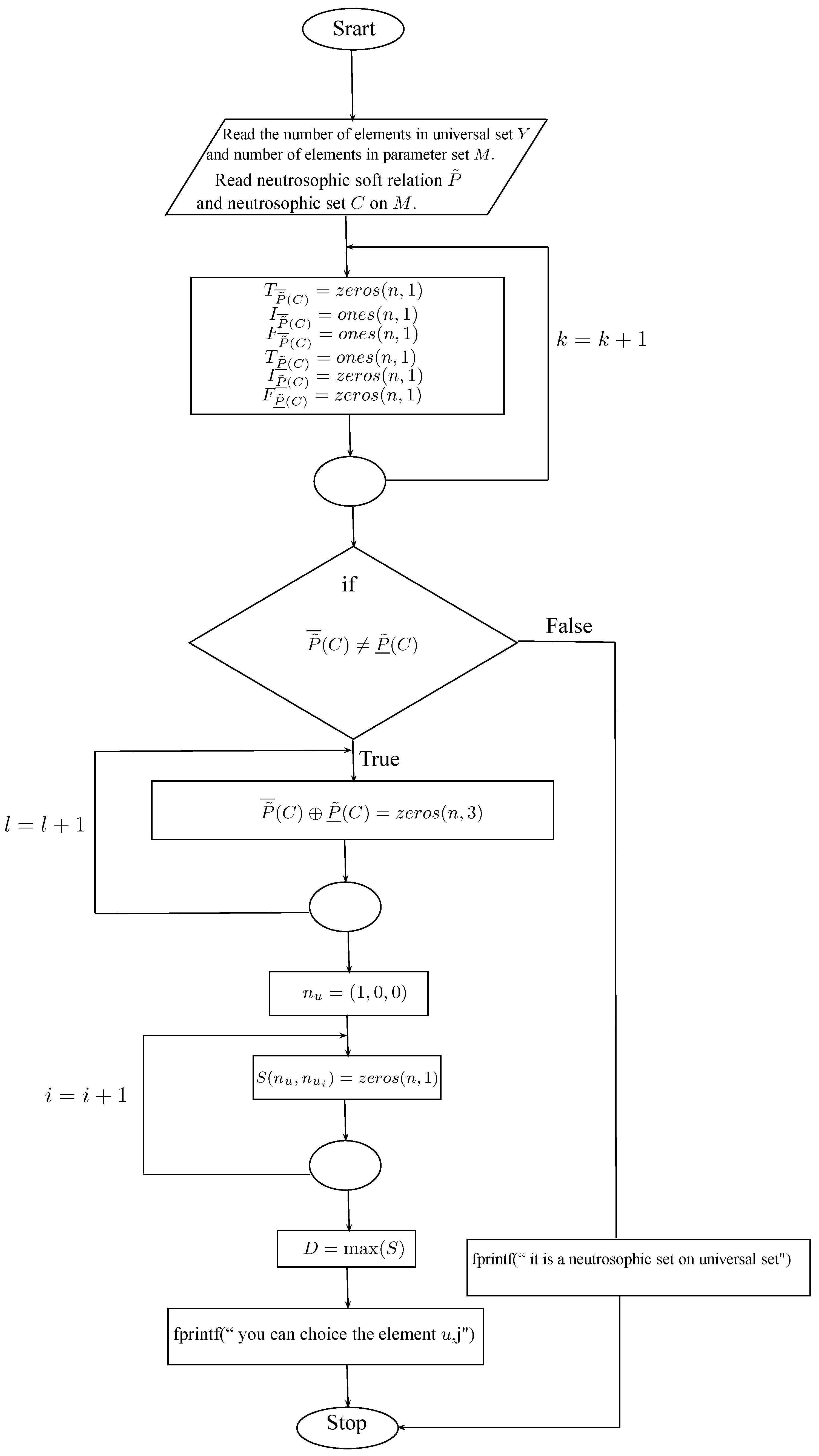
We get Thus, the optimal decision is , and the most suitable generic version of Claritin is Sudafed (Pseudoephedrine). We have used software MATLAB (version 7, MathWorks, Natick, MA, USA) for calculations in the application. The flow chart of the algorithm is general for any number of objects with respect to certain parameters. The flow chart of our proposed method is given in Figure 1. The method is presented as an algorithm in Algorithm 1.
| Algorithm 1: Algorithm for selection of the most suitable objects |
| 1. Begin |
| 2. Input the number of elements in universal set . |
| 3. Input the number of elements in parameter set . |
| 4. Input a neutrosophic soft relation from Y to M. |
| 5. Input an NS C on M. |
| 6. if |
| 7. fprintf(‛ size of neutrosophic soft relation from universal set to parameter |
| set is not correct, it should be of order x) |
| 8. error(‛ Dimemsion of neutrosophic soft relation on vertex set is not correct. ’) |
| 9. end |
| 10. if |
| 11. fprintf(‛ size of NS on parameter set is not correct, |
| it should be of order %dx3; ’,m) |
| 12. error(’Dimemsion of NS on parameter set is not correct.’) |
| 13. end |
| 14. ; |
| 15. ; |
| 16. ; |
| 17. ; |
| 18. ; |
| 19. ; |
| 20. if |
| 21. if |
| 22. if |
| 23. if |
| 24. for |
| 25. for |
| 26. j=3*k-2; |
| 27. ; |
| 28. ; |
| 29. ; |
| 30. ; |
| 31. ; |
| 32. ; |
| 33. end |
| 34. end |
| 35. |
| 36. |
| 37. if |
| 38. fprintf(‛ it is a neutrosophic set on universal set.) |
| 39. else |
| 40. fprintf(‛it is an NSRS on universal set.) |
| 41. ; |
| 42. for i=1:n |
| 43. |
| ; |
| 44. ; |
| 45. ; |
| 46. end |
| 47. ; |
| 48. ; |
| 49. for i=1:n |
| 50. ; |
| 51. end |
| 52. |
| 53. D=max(S); |
| 54. l=0; |
| 55. m=zeros(n,1); |
| 56. D2=zeros(n,1); |
| 57. for j=1:n |
| 58. if S(j,1)==D |
| 59. l=l+1; |
| 60. D2(j,1)=S(j,1); |
| 61. m(j)=j; |
| 62. end |
| 63. end |
| 64. for |
| 65. if |
| 66. fprintf(‛ you can choice the element ,j) |
| 67. end |
| 68. end |
| 69. end |
| 70. end |
| 71. end |
| 72. end |
| 73. end |
| 74. End |
5. Conclusions and Future Directions
Rough set theory can be considered as an extension of classical set theory. Rough set theory is a very useful mathematical model to handle vagueness. NS theory, RS theory and SS theory are three useful distinguished approaches to deal with vagueness. NS and RS models are used to handle uncertainty, and combining these two models with another remarkable model of SSs gives more precise results for decision-making problems. In this paper, we have first presented the notion of SRNSs. Furthermore, we have introduced NSRSs and investigated some properties of NSRSs in detail. The notion of NSRS can be utilized as a mathematical tool to deal with imprecise and unspecified information. In addition, a decision-making method based on NSRSs has been proposed. This research work can be extended to (1) rough bipolar neutrosophic soft sets; (2) bipolar neutrosophic soft rough sets; (3) interval-valued bipolar neutrosophic rough sets; and (4) neutrosophic soft rough graphs.
Author Contributions
Muhammad Akram and Sundas Shahzadi conceived and designed the experiments; Florentin Smarandache analyzed the data; Sundas Shahzadi wrote the paper.
Conflicts of Interest
The authors declare no conflict of interest.
References
- Smarandache, F. Neutrosophy: Neutrosophic Probability, Set, and Logic; American Research Press: Rehoboth, DE, USA, 1998; 105p. [Google Scholar]
- Wang, H.; Smarandache, F.; Zhang, Y.; Sunderraman, R. Single-valued neutrosophic sets. Multispace Multistruct. 2010, 4, 410–413. [Google Scholar]
- Ye, J. Multicriteria decision-making method using the correlation coefficient under single-valued neutrosophic environment. Int. J. Gen. Syst. 2013, 42, 386–394. [Google Scholar] [CrossRef]
- Ye, J. Improved correlation coefficients of single valued neutrosophic sets and interval neutrosophic sets for multiple attribute decision making. J. Intell. Fuzzy Syst. 2014, 27, 2453–2462. [Google Scholar]
- Ye, J.; Fu, J. Multi-period medical diagnosis method using a single valued neutrosophic similarity measure based on tangent function. Comput. Methods Prog. Biomed. 2016, 123, 142–149. [Google Scholar] [CrossRef] [PubMed]
- Peng, J.J.; Wang, J.Q.; Zhang, H.Y.; Chen, X.H. An outranking approach for multi-criteria decision-making problems with simplified neutrosophic sets. Appl. Soft Comput. 2014, 25, 336–346. [Google Scholar] [CrossRef]
- Molodtsov, D.A. Soft set theory-first results. Comput. Math. Appl. 1999, 37, 19–31. [Google Scholar] [CrossRef]
- Maji, P.K.; Biswas, R.; Roy, A.R. Fuzzy soft sets. J. Fuzzy Math. 2001, 9, 589–602. [Google Scholar]
- Maji, P.K.; Biswas, R.; Roy, A.R. Intuitionistic fuzzy soft sets. J. Fuzzy Math. 2001, 9, 677–692. [Google Scholar]
- Maji, P.K. Neutrosophic soft set. Ann. Fuzzy Math. Inform. 2013, 5, 157–168. [Google Scholar]
- Babitha, K.V.; Sunil, J.J. Soft set relations and functions. Comput. Math. Appl. 2010, 60, 1840–1849. [Google Scholar] [CrossRef]
- Sahin, R.; Kucuk, A. On similarity and entropy of neutrosophic soft sets. J. Intell. Fuzzy Syst. Appl. Eng. Technol. 2014, 27, 2417–2430. [Google Scholar]
- Pawlak, Z. Rough sets. Int. J. Comput. Inf. Sci. 1982, 11, 341–356. [Google Scholar] [CrossRef]
- Ali, M. A note on soft sets, rough sets and fuzzy soft sets. Appl. Soft Comput. 2011, 11, 3329–3332. [Google Scholar]
- Feng, F.; Liu, X.; Leoreanu-Fotea, B.; Jun, Y.B. Soft sets and soft rough sets. Inf. Sci. 2011, 181, 1125–1137. [Google Scholar] [CrossRef]
- Shabir, M.; Ali, M.I.; Shaheen, T. Another approach to soft rough sets. Knowl.-Based Syst. 2013, 40, 72–80. [Google Scholar] [CrossRef]
- Feng, F.; Li, C.; Davvaz, B.; Ali, M.I. Soft sets combined with fuzzy sets and rough sets: A tentative approach. Soft Comput. 2010, 14, 899–911. [Google Scholar] [CrossRef]
- Dubois, D.; Prade, H. Rough fuzzy sets and fuzzy rough sets. Int. J. Gen. Syst. 1990, 17, 191–209. [Google Scholar] [CrossRef]
- Meng, D.; Zhang, X.; Qin, K. Soft rough fuzzy sets and soft fuzzy rough sets. Comput. Math. Appl. 2011, 62, 4635–4645. [Google Scholar] [CrossRef]
- Sun, B.Z.; Ma, W.; Liu, Q. An approach to decision making based on intuitionistic fuzzy rough sets over two universes. J. Oper. Res. Soc. 2013, 64, 1079–1089. [Google Scholar] [CrossRef]
- Sun, B.Z.; Ma, W. Soft fuzzy rough sets and its application in decision making. Artif. Intell. Rev. 2014, 41, 67–80. [Google Scholar] [CrossRef]
- Zhang, X.; Dai, J.; Yu, Y. On the union and intersection operations of rough sets based on various approximation spaces. Inf. Sci. 2015, 292, 214–229. [Google Scholar] [CrossRef]
- Zhang, H.; Shu, L. Generalized intuitionistic fuzzy rough set based on intuitionistic fuzzy covering. Inf. Sci. 2012, 198, 186–206. [Google Scholar] [CrossRef]
- Zhang, X.; Zhou, B.; Li, P. A general frame for intuitionistic fuzzy rough sets. Inf. Sci. 2012, 216, 34–49. [Google Scholar] [CrossRef]
- Zhang, H.; Shu, L.; Liao, S. Intuitionistic fuzzy soft rough set and its application in decision making. Abstr. Appl. Anal. 2014, 2014, 13. [Google Scholar]
- Zhang, H.; Xiong, L.; Ma, W. Generalized intuitionistic fuzzy soft rough set and its application in decision making. J. Comput. Anal. Appl. 2016, 20, 750–766. [Google Scholar]
- Broumi, S.; Smarandache, F. Interval-valued neutrosophic soft rough sets. Int. J. Comput. Math. 2015, 2015, 232919. [Google Scholar] [CrossRef]
- Broumi, S.; Smarandache, F.; Dhar, M. Rough Neutrosophic sets. Neutrosophic Sets Syst. 2014, 3, 62–67. [Google Scholar]
- Yang, H.L.; Zhang, C.L.; Guo, Z.L.; Liu, Y.L.; Liao, X. A hybrid model of single valued neutrosophic sets and rough sets: Single valued neutrosophic rough set model. Soft Comput. 2016, 21, 6253–6267. [Google Scholar] [CrossRef]
- Faizi, S.; Salabun, W.; Rashid, T.; Watrbski, J.; Zafar, S. Group decision-making for hesitant fuzzy sets based on characteristic objects method. Symmetry 2017, 9, 136. [Google Scholar] [CrossRef]
- Faizi, S.; Rashid, T.; Salabun, W.; Zafar, S.; Watrbski, J. Decision making with uncertainty using hesitant fuzzy sets. Int. J. Fuzzy Syst. 2018, 20, 93–103. [Google Scholar] [CrossRef]
- Mardani, A.; Nilashi, M.; Antucheviciene, J.; Tavana, M.; Bausys, R.; Ibrahim, O. Recent Fuzzy Generalisations of Rough Sets Theory: A Systematic Review and Methodological Critique of the Literature. Complexity 2017, 2017, 33. [Google Scholar] [CrossRef]
- Liang, R.X.; Wang, J.Q.; Zhang, H.Y. A multi-criteria decision-making method based on single-valued trapezoidal neutrosophic preference relations with complete weight information. Neural Comput. Appl. 2017, 1–16. [Google Scholar] [CrossRef]
- Liang, R.; Wang, J.; Zhang, H. Evaluation of e-commerce websites: An integrated approach under a single-valued trapezoidal neutrosophic environment. Knowl.-Based Syst. 2017, 135, 44–59. [Google Scholar] [CrossRef]
- Peng, H.G.; Zhang, H.Y.; Wang, J.Q. Probability multi-valued neutrosophic sets and its application in multi-criteria group decision-making problems. Neural Comput. Appl. 2016, 1–21. [Google Scholar] [CrossRef]
- Wang, L.; Zhang, H.Y.; Wang, J.Q. Frank Choquet Bonferroni mean operators of bipolar neutrosophic sets and their application to multi-criteria decision-making problems. Int. J. Fuzzy Syst. 2018, 20, 13–28. [Google Scholar] [CrossRef]
- Zavadskas, E.K.; Bausys, R.; Kaklauskas, A.; Ubarte, I.; Kuzminske, A.; Gudiene, N. Sustainable market valuation of buildings by the single-valued neutrosophic MAMVA method. Appl. Soft Comput. 2017, 57, 74–87. [Google Scholar] [CrossRef]
- Li, Y.; Liu, P.; Chen, Y. Some single valued neutrosophic number heronian mean operators and their application in multiple attribute group decision making. Informatica 2016, 27, 85–110. [Google Scholar] [CrossRef]
Figure 1.
Flow chart for selection of most suitable objects.

Table 1.
Crisp soft relation P.
| P | |||||
|---|---|---|---|---|---|
Table 2.
Soft set .
| P | |||
|---|---|---|---|
Table 3.
Soft relation R.
| R | ||||
|---|---|---|---|---|
Table 4.
Neutrosophic soft relation .
Table 5.
Neutrosophic soft set .
Table 6.
Neutrosophic soft relation .
Table 7.
Neutrosophic soft set .
© 2018 by the authors. Licensee MDPI, Basel, Switzerland. This article is an open access article distributed under the terms and conditions of the Creative Commons Attribution (CC BY) license (http://creativecommons.org/licenses/by/4.0/).
Share and Cite
MDPI and ACS Style
Akram, M.; Shahzadi, S.; Smarandache, F. Multi-Attribute Decision-Making Method Based on Neutrosophic Soft Rough Information. Axioms 2018, 7, 19. https://doi.org/10.3390/axioms7010019
AMA Style
Akram M, Shahzadi S, Smarandache F. Multi-Attribute Decision-Making Method Based on Neutrosophic Soft Rough Information. Axioms. 2018; 7(1):19. https://doi.org/10.3390/axioms7010019
Chicago/Turabian StyleAkram, Muhammad, Sundas Shahzadi, and Florentin Smarandache. 2018. "Multi-Attribute Decision-Making Method Based on Neutrosophic Soft Rough Information" Axioms 7, no. 1: 19. https://doi.org/10.3390/axioms7010019
Note that from the first issue of 2016, this journal uses article numbers instead of page numbers. See further details here.