Cross Entropy Measures of Bipolar and Interval Bipolar Neutrosophic Sets and Their Application for Multi-Attribute Decision-Making

Abstract

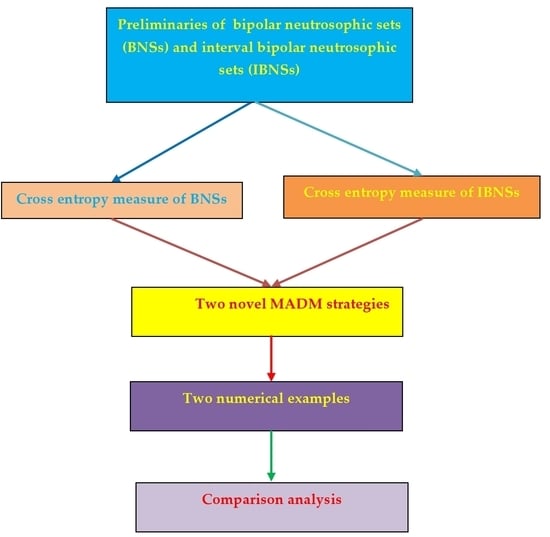
The bipolar neutrosophic set is an important extension of the bipolar fuzzy set. The bipolar neutrosophic set is a hybridization of the bipolar fuzzy set and neutrosophic set. Every element of a bipolar neutrosophic set consists of three independent positive membership functions and three independent negative membership functions. In this paper, we develop cross entropy measures of bipolar neutrosophic sets and prove their basic properties. We also define cross entropy measures of interval bipolar neutrosophic sets and prove their basic properties. Thereafter, we develop two novel multi-attribute decision-making strategies based on the proposed cross entropy measures. In the decision-making framework, we calculate the weighted cross entropy measures between each alternative and the ideal alternative to rank the alternatives and choose the best one. We solve two illustrative examples of multi-attribute decision-making problems and compare the obtained result with the results of other existing strategies to show the applicability and effectiveness of the developed strategies. At the end, the main conclusion and future scope of research are summarized.

1. Introduction

Shannon and Weaver [1] and Shannon [2] proposed the entropy measure which dealt formally with communication systems at its inception. According to Shannon and Weaver [1] and Shannon [2], the entropy measure is an important decision-making apparatus for computing uncertain information. Shannon [2] introduced the concept of the cross entropy strategy in information theory.

The measure of a quantity of fuzzy information obtained from a fuzzy set or fuzzy system is termed fuzzy entropy. However, the meaning of fuzzy entropy is quite different from the classical Shannon entropy because it is defined based on a nonprobabilistic concept [3,4,5], while Shannon entropy is defined based on a randomness (probabilistic) concept. In 1968, Zadeh [6] extended the Shannon entropy to fuzzy entropy on a fuzzy subset with respect to the concerned probability distribution. In 1972, De Luca and Termini [7] proposed fuzzy entropy based on Shannon’s function and introduced the axioms with which the fuzzy entropy should comply. Sander [8] presented Shannon fuzzy entropy and proved that the properties sharpness, valuation, and general additivity have to be imposed on fuzzy entropy. Xie and Bedrosian [9] proposed another form of total fuzzy entropy. To overcome the drawbacks of total entropy [8,9], Pal and Pal [10] introduced hybrid entropy that can be used as an objective measure for a proper defuzzification of a certain fuzzy set. Hybrid entropy [10] considers both probabilistic entropies in the absence of fuzziness. In the same study, Pal and Pal [10] defined higher-order entropy. Kaufmann and Gupta [11] studied the degree of fuzziness of a fuzzy set by a metric distance between its membership function and the membership function (characteristic function) of its nearest crisp set. Yager [12,13] introduced a fuzzy entropy card as a fuzziness measure by observing that the intersection of a fuzzy set and its complement is not the void set. Kosko [14,15] studied the fuzzy entropy of a fuzzy set based on the fuzzy set geometry and distances between them. Parkash et al. [16] proposed two new measures of weighted fuzzy entropy.

Burillo and Bustince [17] presented an axiomatic definition of an intuitionistic fuzzy entropy measure. Szmidt and Kacprzyk [18] developed a new entropy measure based on a geometric interpretation of the intuitionistic fuzzy set (IFS). Wei et al. [19] proposed an entropy measure for interval-valued intuitionistic fuzzy sets (IVIFSs) and employed it in pattern recognition and multi criteria decision-making (MCDM). Li [20] presented a new multi-attribute decision-making (MADM) strategy combining entropy and technique for order of preference by similarity to ideal solution (TOPSIS) in the IVIFS environment.

Shang and Jiang [21] developed cross entropy in the fuzzy environment. Vlachos and Sergiadis [22] presented intuitionistic fuzzy cross entropy by extending fuzzy cross entropy [21]. Ye [23] proposed a new cross entropy in the IVIFS environment and developed an optimal decision-making strategy. Xia and Xu [24] defined a new entropy and a cross entropy and presented multi-attribute group decision-making (MAGDM) strategy in the IFS environment. Tong and Yu [25] defined cross entropy in the IVIFS environment and employed it to solve MADM problems.

Smarandache [26] introduced the neutrosophic set, which is a generalization of the fuzzy set [27] and intuitionistic fuzzy set [28]. The single-valued neutrosophic set (SVNS) [29], an instance of the neutrosophic set, has caught the attention of researchers due to its applicability in decision-making [30,31,32,33,34,35,36,37,38,39,40,41,42,43,44,45,46,47,48,49,50,51,52,53,54,55,56,57,58,59,60,61], conflict resolution [62], educational problems [63,64], image processing [65,66,67], cluster analysis [68,69], social problems [70,71], etc.

Majumdar and Samanta [72] proposed an entropy measure and presented an MCDM strategy in the SVNS environment. Ye [73] defined cross entropy for SVNS and proposed an MCDM strategy which bears undefined phenomena. To overcome the undefined phenomena, Ye [74] defined improved cross entropy measures for SVNSs and interval neutrosophic sets (INSs) [75], which are straightforward symmetric, and employed them to solve MADM problems. Since MADM strategies [73,74] are suitable for single-decision-maker-oriented problems, Pramanik et al. [76] defined NS-cross entropy and developed an MAGDM strategy which is straightforward symmetric and free from undefined phenomena and suitable for group decision making problem. Şahin [77] proposed two techniques to convert the interval neutrosophic information to single-valued neutrosophic information and fuzzy information. In the same study, Şahin [77] defined an interval neutrosophic cross entropy measure by utilizing two reduction methods and an MCDM strategy. Tian et al. [78] developed a transformation operator to convert interval neutrosophic numbers to single-valued neutrosophic numbers and defined cross entropy measures for two SVNSs. In the same study, Tian et al. [78] developed an MCDM strategy based on cross entropy and TOPSIS [79] where the weight of the criterion is incomplete. Tian et al. [78] defined a cross entropy for INSs and developed an MCDM strategy based on the cross entropy and TOPSIS. The MCDM strategies proposed by Sahin [77] and Tian et al. [78] are applicable for a single decision maker only. Therefore, multiple decision-makers cannot participate in the strategies in [77,78]. To tackle the problem, Dalapati et al. [80] proposed IN-cross entropy and weighted IN-cross entropy and developed an MAGDM strategy.

Deli et al. [81] proposed bipolar neutrosophic set (BNS) by hybridizing the concept of bipolar fuzzy sets [82,83] and neutrosophic sets [26]. A BNS has two fully independent parts, which are positive membership degree T⁺ $\to$ [0, 1], I⁺ $\to$ [0, 1], F⁺ $\to$ [0, 1], and negative membership degree T⁻ $\to$ [−1, 0], I⁻ $\to$ [−1, 0], F⁻ $\to$ [−1, 0], where the positive membership degrees T⁺, I⁺, F⁺ represent truth membership degree, indeterminacy membership degree, and false membership degree, respectively, of an element and the negative membership degrees T⁻, I⁻, F⁻ represent truth membership degree, indeterminacy membership degree, and false membership degree, respectively, of an element to some implicit counter property corresponding to a BNS. Deli et al. [81] defined some operations, namely, score, accuracy, and certainty functions, to compare BNSs and provided some operators in order to aggregate BNSs. Deli and Subas [84] defined a correlation coefficient similarity measure for dealing with MCDM problems in a single-valued bipolar neutrosophic setting. Şahin et al. [85] proposed a Jaccard vector similarity measure for MCDM problems with single-valued neutrosophic information. Uluçay et al. [86] introduced a Dice similarity measure, weighted Dice similarity measure, hybrid vector similarity measure, and weighted hybrid vector similarity measure for BNSs and established an MCDM strategy. Dey et al. [87] investigated a TOPSIS strategy for solving multi-attribute decision-making (MADM) problems with bipolar neutrosophic information where the weights of the attributes are completely unknown to the decision-maker. Pramanik et al. [88] defined projection, bidirectional projection, and hybrid projection measures for BNSs and proved their basic properties. In the same study, Pramanik et al. [88] developed three new MADM strategies based on the proposed projection, bidirectional projection, and hybrid projection measures with bipolar neutrosophic information. Wang et al. [89] defined Frank operations of bipolar neutrosophic numbers (BNNs) and proposed Frank bipolar neutrosophic Choquet Bonferroni mean operators by combining Choquet integral operators and Bonferroni mean operators based on Frank operations of BNNs. In the same study, Wang et al. [89] established an MCDM strategy based on Frank Choquet Bonferroni operators of BNNs in a bipolar neutrosophic environment. Pramanik et al. [90] developed a Tomada de decisao interativa e multicritévio (TODIM) strategy for MAGDM in a bipolar neutrosophic environment. An MADM strategy based on cross entropy for BNSs is yet to appear in the literature.

Mahmood et al. [91] and Deli et al. [92] introduced the hybridized structure called interval bipolar neutrosophic sets (IBNSs) by combining BNSs and INSs and defined some operations and operators for IBNSs. An MADM strategy based on cross entropy for IBNSs is yet to appear in the literature.

Research gap:

An MADM strategy based on cross entropy for BNSs and an MADM strategy based on cross entropy for IBNSs.

This paper answers the following research questions:

• Is it possible to define a new cross entropy measure for BNSs?
• Is it possible to define a new weighted cross entropy measure for BNSs?
• Is it possible to develop a new MADM strategy based on the proposed cross entropy measure in a BNS environment?
• Is it possible to develop a new MADM strategy based on the proposed weighted cross entropy measure in a BNS environment?
• Is it possible to define a new cross entropy measure for IBNSs?
• Is it possible to define a new weighted cross entropy measure for IBNSs?
• Is it possible to develop a new MADM strategy based on the proposed cross entropy measure in an IBNS environment?
• Is it possible to develop a new MADM strategy based on the proposed weighted cross entropy measure in an IBNS environment?

Motivation:

The above-mentioned analysis presents the motivation behind proposing a cross-entropy-based strategy for tackling MADM in BNS and IBNS environments. This study develops two novel cross-entropy-based MADM strategies.

The objectives of the paper are:

• To define a new cross entropy measure and prove its basic properties.
• To define a new weighted cross measure and prove its basic properties.
• To develop a new MADM strategy based on the weighted cross entropy measure in a BNS environment.
• To develop a new MADM strategy based on the weighted cross entropy measure in an IBNS environment.

To fill the research gap, we propose a cross-entropy-based MADM strategy in the BNS environment and the IBNS environment.

The main contributions of this paper are summarized below:

• We propose a new cross entropy measure in the BNS environment and prove its basic properties.
• We propose a new weighted cross entropy measure in the IBNS environment and prove its basic properties.
• We develop a new MADM strategy based on weighted cross entropy to solve MADM problems in a BNS environment.
• We develop a new MADM strategy based on weighted cross entropy to solve MADM problems in an IBNS environment.
• Two illustrative numerical examples are solved and a comparison analysis is provided.

The rest of the paper is organized as follows. In Section 2, we present some concepts regarding SVNSs, INSs, BNSs, and IBNSs. Section 3 proposes cross entropy and weighted cross entropy measures for BNSs and investigates their properties. In Section 4, we extend the cross entropy measures for BNSs to cross entropy measures for IBNSs and discuss their basic properties. Two novel MADM strategies based on the proposed cross entropy measures in bipolar and interval bipolar neutrosophic settings are presented in Section 5. In Section 6, two numerical examples are solved and a comparison with other existing methods is provided. In Section 7, conclusions and the scope of future work are provided.

2. Preliminary

In this section, we provide some basic definitions regarding SVNSs, INSs, BNSs, and IBNSs.

2.1. Single-Valued Neutrosophic Sets

An SVNS [29] S in U is characterized by a truth membership function $T_S(x)$, an indeterminate membership function $I_S(x)$, and a falsity membership function $F_S(x)$. An SVNS S over U is defined by

$$S=\{x,\hspace{0.17em}\langle T_S(x),I_S(x),\hspace{0.17em}{F}_S(x)\rangle |x\in U\}$$

where, $T_S(x),I_S(x),\hspace{0.17em}{F}_S(x)$: U → [0, 1] and 0 $\le$ $T_S(x)+I_S(x)+F_S(x)$ $\le$ 3 for each point x ∈ U.

2.2. Interval Neutrosophic Set

An interval neutrosophic set [75] P in U is expressed as given below:

$$\begin{array}{l}P=\{x,\hspace{0.17em}\langle T_P(x),I_P(x),\hspace{0.17em}{F}_P(x)\rangle |x\in U\}\\ \hspace{0.17em}\hspace{0.17em}\hspace{0.17em}=\{x,\hspace{0.17em}\left[\inf T_p(x), \sup T_p(x)\right]; \left[\inf I_p(x), \sup I_p(x)\right]; \left[\inf F_p(x) \sup F_p(x)\right]|x\in U\}\end{array}$$

where $T_P(x)$, $I_P(x)$, $F_P(x)$ are the truth membership function, indeterminacy membership function, and falsity membership function, respectively. For each point x in U, $T_P(x)$, $I_P(x)$, $F_P(x)$ $\subseteq$ [0, 1] satisfying the condition 0 $\le$ sup $T_P(x)$ + sup $I_P(x)$ + sup $F_P(x)$ $\le$ 3.

2.3. Bipolar Neutrosophic Set

A BNS [81] E in U is presented as given below:

$$E= \{x,\langle T_E^{+}(x),I_E^{+}(x),\hspace{0.17em}{F}_E^{+}(x),\hspace{0.17em}{T}_E^{-}(x), I_E^{-}(x), F_E^{-}(x)\rangle |x\in U\}$$

where $T_E^{+}(x)$, $I_E^{+}(x)$, $F_E^{+}(x)$: U → [0, 1] and $T_E^{-}(x)$, $I_E^{-}(x)$, $F_E^{-}(x)$: U → [−1, 0]. Here, $T_E^{+}(x)$, $I_E^{+}(x)$, $F_E^{+}(x)$ denote the truth membership, indeterminate membership, and falsity membership functions corresponding to BNS E on an element x ∈ U, and $T_E^{-}(x)$, $I_E^{-}(x)$, $F_E^{-}(x)$ denote the truth membership, indeterminate membership, and falsity membership of an element x ∈ U to some implicit counter property corresponding to E.

Definition 1.

Ref. [81]: Let, E₁ = {x, $\langle T_{E_1}^{+}(x),I_{E_1}^{+}(x),\hspace{0.17em}{F}_{E_1}^{+}(x),\hspace{0.17em}{T}_{E_1}^{-}(x), I_{E_1}^{-}(x), F_{E_1}^{-}(x)\rangle$ |x ∈ U} and E₂ = {x, $\langle T_{E_2}^{+}(x),I_{E_2}^{+}(x),\hspace{0.17em}{F}_{E_2}^{+}(x),\hspace{0.17em}{T}_{E_2}^{-}(x), I_{E_2}^{-}(x), F_{E_2}^{-}(x)\rangle$ |x ∈ X} be any two BNSs. Then

• E₁$\subseteq$E₂ if, and only if,

$T_{E_1}^{+}(x)$$\le$$T_{E_2}^{+}(x)$,$I_{E_1}^{+}(x)$$\le$$I_{E_2}^{+}(x)$,$F_{E_1}^{+}(x)$$\ge$$F_{E_2}^{+}(x)$;$T_{E_1}^{-}(x)$$\ge$$T_{E_2}^{-}(x)$,$I_{E_1}^{-}(x)$$\ge$$I_{E_2}^{-}(x)$,$F_{E_1}^{-}(x)$$\le$$F_{E_2}^{-}(x)$for all x ∈ U.

• E₁ = E₂ if, and only if,

$T_{E_1}^{+}(x)$=$T_{E_2}^{+}(x)$,$I_{E_1}^{+}(x)$=$I_{E_2}^{+}(x)$,$F_{E_1}^{+}(x)$=$F_{E_2}^{+}(x)$;$T_{E_1}^{-}(x)$=$T_{E_2}^{-}(x)$,$I_{E_1}^{-}(x)$=$I_{E_2}^{-}(x)$,$F_{E_1}^{-}(x)$=$F_{E_2}^{-}(x)$for all x ∈ U.

• The complement of E is E^c = {x,$\langle T_{E^{\mathrm{c}}}^{+}(x),I_{E^{\mathrm{c}}}^{+}(x),\hspace{0.17em}{F}_{E^{\mathrm{c}}}^{+}(x),\hspace{0.17em}{T}_{E^{\mathrm{c}}}^{-}(x), I_{E^{\mathrm{c}}}^{-}(x), F_{E^{\mathrm{c}}}^{-}(x)\rangle$|x ∈ U}

where

$$T_{E^{\mathrm{c}}}^{+}(x)\hspace{0.17em}=\hspace{0.17em}{F}_E^{+}(x),\hspace{0.17em}{I}_{E^{\mathrm{c}}}^{+}(x)\hspace{0.17em}=\hspace{0.17em}1\hspace{0.17em}-I_E^{+}(x),\hspace{0.17em}{F}_{E^{\mathrm{c}}}^{+}(x)\hspace{0.17em}=\hspace{0.17em}{T}_E^{+}(x);$$

$$T_{E^{\mathrm{c}}}^{-}(x)\hspace{0.17em}=\hspace{0.17em}{F}_E^{-}(x),\hspace{0.17em}{I}_{E^{\mathrm{c}}}^{-}(x)\hspace{0.17em}=\hspace{0.17em}-1-\hspace{0.17em}{I}_E^{-}(x),\hspace{0.17em}{F}_{E^{\mathrm{c}}}^{-}(x)\hspace{0.17em}=\hspace{0.17em}{T}_E^{-}(x).$$

• The union E₁$\cup$E₂ is defined as follows:

E₁$\cup$E₂ = {Max ($T_{E_1}^{+}(x)$,$T_{E_2}^{+}(x)$), Min ($I_{E_1}^{+}(x)$,$I_{E_2}^{+}(x)$), Min ($F_{E_1}^{+}(x)$,$F_{E_2}^{+}(x)$), Min ($T_{E_1}^{-}(x)$,$T_{E_2}^{-}(x)$), Max ($I_{E_1}^{-}(x)$,$I_{E_2}^{-}(x)$), Max ($F_{E_1}^{-}(x)$,$F_{E_2}^{-}(x)$)},$\forall$x ∈ U.

• The intersection E₁$\cap$E₂ [88] is defined as follows:

E₁$\cap$E₂ = {Min ($T_{E_1}^{+}(x)$,$T_{E_2}^{+}(x)$), Max ($I_{E_1}^{+}(x)$,$I_{E_2}^{+}(x)$), Max ($F_{E_1}^{+}(x)$,$F_{E_2}^{+}(x)$), Max ($T_{E_1}^{-}(x)$,$T_{E_2}^{-}(x)$), Min ($I_{E_1}^{-}(x)$,$I_{E_2}^{-}(x)$), Min ($F_{E_1}^{-}(x)$,$F_{E_2}^{-}(x)$)},$\forall$x ∈ U.

2.4. Interval Bipolar Neutrosophic Sets

An IBNS [91,92] R = {x, <[inf$T_R^{+}$(x), sup$T_R^{+}$(x)]; [inf$I_R^{+}$(x), sup$I_R^{+}$(x)]; [inf$F_R^{+}$(x), sup$F_R^{+}$(x)]; [inf$T_R^{-}$(x), sup$T_R^{-}$(x)]; [inf$I_R^{-}$(x), sup$I_R^{-}$(x)]; [inf$F_R^{-}$(x), sup$F_R^{-}$(x)]>|x ∈ U} is characterized by positive and negative truth membership functions $T_R^{+}$(x), $T_R^{-}$(x), respectively; positive and negative indeterminacy membership functions $I_R^{+}$(x), $I_R^{-}$(x), respectively; and positive and negative falsity membership functions $F_R^{+}$(x), $F_R^{-}$(x), respectively. Here, for any x ∈ U, $T_R^{+}$(x), $I_R^{+}$(x), $F_R^{+}$(x) $\subseteq$ [0, 1] and $T_R^{-}$(x), $I_R^{-}$(x), $F_R^{-}$(x) $\subseteq$ [−1, 0] with the conditions 0 $\le$ sup$T_R^{+}$(x) + sup$I_R^{+}$(x) + sup$F_R^{+}$(x) $\le$ 3 and −3 $\le$ sup$T_R^{-}$(x) + sup$I_R^{-}$(x) + sup$F_R^{-}$(x) $\le$ 0.

Definition 2.

Ref. [91,92]: Let R = {x, <[inf$T_R^{+}$(x), sup$T_R^{+}$(x)]; [inf$I_R^{+}$(x), sup$I_R^{+}$(x)]; [inf$F_R^{+}$(x), sup$F_R^{+}$(x)]; [inf$T_R^{-}$(x), sup$T_R^{-}$(x)]; [inf$I_R^{-}$(x), sup$I_R^{-}$(x)]; [inf$F_R^{-}$(x), sup$F_R^{-}$(x)]>|x ∈ U} and S = {x, <[inf$T_S^{+}$(x), sup$T_S^{+}$(x)]; [inf$I_S^{+}$(x), sup$I_S^{+}$(x)]; [inf$F_S^{+}$(x), sup$F_S^{+}$(x)]; [inf$T_S^{-}$(x), sup$T_S^{-}$(x)]; [inf$I_S^{-}$(x), sup$I_S^{-}$(x)]; [inf$F_S^{-}$(x), sup$F_S^{-}$(x)]>|x ∈ U} be two IBNSs in U. Then

• R$\subseteq$S if, and only if,
  inf$T_R^{+}$(x)$\le$inf$T_S^{+}$(x), sup$T_R^{+}$(x)$\le$sup$T_S^{+}$(x),
  inf$I_R^{+}$(x)$\ge$inf$I_S^{+}$(x), sup$I_R^{+}$(x)$\ge$sup$I_S^{+}$(x),
  inf$F_R^{+}$(x)$\ge$inf$F_S^{+}$(x), sup$F_R^{+}$(x)$\ge$sup$F_S^{+}$(x),
  inf$T_R^{-}$(x)$\ge$inf$T_S^{-}$(x), sup$T_R^{-}$(x)$\ge$sup$T_S^{-}$(x),
  inf$I_R^{-}$(x)$\le$inf$I_S^{-}$(x), sup$I_R^{-}$(x)$\le$sup$I_S^{-}$(x),
  inf$F_R^{-}$(x)$\le$inf$F_S^{-}$(x), sup$F_R^{-}$(x)$\le$sup$F_S^{-}$(x),
  for all x ∈ U.
• R = S if, and only if,
  inf$T_R^{+}$(x) = inf$T_S^{+}$(x), sup$T_R^{+}$(x) = sup$T_S^{+}$(x), inf$I_R^{+}$(x) = inf$I_S^{+}$(x), sup$I_R^{+}$(x) = sup$I_S^{+}$(x),
  inf$F_R^{+}$(x) = inf$F_S^{+}$(x), sup$F_R^{+}$(x) = sup$F_S^{+}$(x), inf$T_R^{-}$(x) = inf$T_S^{-}$(x), sup$T_R^{-}$(x) = sup$T_S^{-}$(x),
  inf$I_R^{-}$(x) = inf$I_S^{-}$(x), sup$I_R^{-}$(x) = sup$I_S^{-}$(x), inf$F_R^{-}$(x) = inf$F_S^{-}$(x), sup$F_R^{-}$(x) = sup$F_S^{-}$(x),
  for all x ∈ U.
• The complement of R is defined as The complement of R is defined as R^C = {x, < [inf $T_{R^C}^{+}$(x), sup$T_{R^C}^{+}$(x)]; [inf$I_{R^C}^{+}$(x), sup$I_{R^C}^{+}$(x)]; [inf$F_{R^C}^{+}$(x), sup$F_{R^C}^{+}$(x)]; [inf$T_{R^C}^{-}$(x), sup$T_{R^C}^{-}$(x)]; [inf$I_{R^C}^{-}$(x), sup$I_{R^C}^{-}$(x)]; [inf $F_{R^C}^{-}$(x), sup$F_{R^C}^{-}$(x)] > | x∈ U} where
  inf $T_{R^C}^{+}$(x) = inf$F_R^{+}$(x), sup$T_{R^C}^{+}$(x) = sup$F_R^{+}$(x)
  inf $I_{R^C}^{+}$(x) = 1 − sup$I_R^{+}$(x), sup$I_{R^C}^{+}$(x) = 1 − inf$I_R^{+}$(x)
  inf$F_{R^C}^{+}$(x) = inf$T_R^{+}$, sup$F_{R^C}^{+}$(x) = sup$T_R^{+}$
  inf$T_{R^C}^{-}$(x) = inf$F_R^{-}$, sup$T_{R^C}^{-}$(x) = sup$F_R^{-}$
  inf$I_{R^C}^{-}$(x) = −1 − sup$I_R^{-}$(x), sup$I_{R^C}^{-}$(x) = −1 − inf$I_R^{-}$(x)
  inf$F_{R^C}^{-}$(x) = inf$T_R^{-}$ (x), sup$F_{R^C}^{-}$(x) = sup$T_R^{-}$ (x)
  for all x∈ U.

3. Cross Entropy Measures of Bipolar Neutrosophic Sets

In this section we define a cross entropy measure between two BNSs and establish some of its basic properties.

Definition 3.

For any two BNSs M and N in U, the cross entropy measure can be defined as follows.

$$C_B\left(M,N\right) ={\displaystyle \sum _{i=1}^n\left[\begin{array}{c}\sqrt{\frac{T_M^{+}\left(x_i\right)+T_N^{+}\left(x_i\right)}{2}}-\left(\frac{\sqrt{T_M^{+}\left(x_i\right)}+\sqrt{T_N^{+}\left(x_i\right)}}{2}\right)+\sqrt{\frac{I_M^{+}\left(x_i\right)+I_N^{+}\left(x_i\right)}{2}}-\left(\frac{\sqrt{I_M^{+}\left(x_i\right)}+\sqrt{I_N^{+}\left(x_i\right)}}{2}\right)+\hfill \\ \sqrt{\frac{(1-I_M^{+}(x_i\left)\right)+(1-I_N^{+}(x_i\left)\right)}{2}}-\left(\frac{\sqrt{(1-I_M^{+}(x_i\left)\right)}+\sqrt{(1-I_N^{+}(x_i\left)\right)}}{2}\right)+\sqrt{\frac{F_M^{+}\left(x_i\right)+F_N^{+}\left(x_i\right)}{2}}-\left(\frac{\sqrt{F_M^{+}\left(x_i\right)}+\sqrt{F_N^{+}\left(x_i\right)}}{2}\right)+\\ \sqrt{\frac{-\left(T_M^{-}\right(x_i)+T_N^{-}(x_i\left)\right)}{2}}-\left(\frac{\sqrt{(-T_M^{-}(x_i\left)\right)}+\sqrt{(-T_N^{-}(x_i\left)\right)}}{2}\right)+\sqrt{\frac{-\left(I_M^{-}\right(x_i)+I_N^{-}(x_i\left)\right)}{2}}-\left(\frac{\sqrt{(-I_M^{-}(x_i\left)\right)}+\sqrt{(-I_N^{-}(x_i\left)\right)}}{2}\right)+\\ \sqrt{\frac{(1+I_M^{-}(x_i\left)\right)+(1+I_N^{-}(x_i\left)\right)}{2}}-\left(\frac{\sqrt{1+I_M^{-}\left(x_i\right)}+\sqrt{1+I_N^{-}\left(x_i\right)}}{2}\right)+\sqrt{\frac{-\left(F_M^{-}\right(x_i)+F_N^{-}(x_i\left)\right)}{2}}-\left(\frac{\sqrt{(-F_M^{-}(x_i\left)\right)}+\sqrt{(-F_N^{-}(x_i\left)\right)}}{2}\right)\end{array}\right]}$$

(1)

Theorem 1.

If M = <$T_M^{+}(x_i)$,$I_M^{+}(x_i)$,$F_M^{+}(x_i)$,$T_M^{-}(x_i)$,$I_M^{-}(x_i)$,$F_M^{-}(x_i)$> and N <$T_N^{+}(x_i)$,$I_N^{+}(x_i)$,$F_N^{+}(x_i)$,$T_N^{-}(x_i)$,$I_N^{-}(x_i)$,$F_N^{-}(x_i)$> are two BNSs in U, then the cross entropy measure C_B(M, N) satisfies the following properties:

(1)

C_B(M, N)$\ge$0;

(2)

C_B(M, N) = 0 if, and only if,$T_M^{+}(x_i)$=$T_N^{+}(x_i)$,$I_M^{+}(x_i)$=$I_N^{+}(x_i)$,$F_M^{+}(x_i)$=$F_N^{+}(x_i)$,$T_M^{-}(x_i)$=$T_N^{-}(x_i)$,$I_M^{-}(x_i)$=$I_N^{-}(x_i)$,$F_M^{-}(x_i)$=$F_N^{-}(x_i)$,$\forall$x ∈ U;

(3)

C_B(M, N) = C_B(N, M);

(4)

C_B(M, N) = C_B(M^C, N^C).

Proof 

(1)

We have the inequality ${\left(\frac{a+b}{2}\right)}^{\raisebox{1ex}{$1$}\!\left/ \!\raisebox{-1ex}{$2$}\right.}\ge \frac{a^{\raisebox{1ex}{$1$}\!\left/ \!\raisebox{-1ex}{$2$}\right.}+b^{\raisebox{1ex}{$1$}\!\left/ \!\raisebox{-1ex}{$2$}\right.}}{2}$ for all positive numbers a and b. From the inequality we can easily obtain C_B(M, N) $\ge$ 0.

(2)

The inequality ${\left(\frac{a+b}{2}\right)}^{\raisebox{1ex}{$1$}\!\left/ \!\raisebox{-1ex}{$2$}\right.}\ge \frac{a^{\raisebox{1ex}{$1$}\!\left/ \!\raisebox{-1ex}{$2$}\right.}+b^{\raisebox{1ex}{$1$}\!\left/ \!\raisebox{-1ex}{$2$}\right.}}{2}$ becomes the equality ${\left(\frac{a+b}{2}\right)}^{\raisebox{1ex}{$1$}\!\left/ \!\raisebox{-1ex}{$2$}\right.}=\frac{a^{\raisebox{1ex}{$1$}\!\left/ \!\raisebox{-1ex}{$2$}\right.}+b^{\raisebox{1ex}{$1$}\!\left/ \!\raisebox{-1ex}{$2$}\right.}}{2}$ if, and only if, a = b and therefore C_B(M, N) = 0 if, and only if, M = N, i.e., $T_M^{+}(x_i)$ = $T_N^{+}(x_i)$, $I_M^{+}(x_i)$ = $I_N^{+}(x_i)$, $F_M^{+}(x_i)$ = $F_N^{+}(x_i)$, $T_M^{-}(x_i)$ = $T_N^{-}(x_i)$, $I_M^{-}(x_i)$ = $I_N^{-}(x_i)$, $F_M^{-}(x_i)$ = $F_N^{-}(x_i)$ $\forall$ x ∈ U.

(3)

C_B(M, N) = ${\displaystyle \sum _{i=1}^n}$$\left[\begin{array}{l}\sqrt{\frac{T_M^{+}\left(x_i\right)+T_N^{+}\left(x_i\right)}{2}}-\left(\frac{\sqrt{T_M^{+}\left(x_i\right)}+\sqrt{T_N^{+}\left(x_i\right)}}{2}\right)+\sqrt{\frac{I_M^{+}\left(x_i\right)+I_N^{+}\left(x_i\right)}{2}}-\left(\frac{\sqrt{I_M^{+}\left(x_i\right)}+\sqrt{I_N^{+}\left(x_i\right)}}{2}\right)+\\ \sqrt{\frac{(1-I_M^{+}(x_i\left)\right)+(1-I_N^{+}(x_i\left)\right)}{2}}-\left(\frac{\sqrt{(1-I_M^{+}(x_i\left)\right)}+\sqrt{(1-I_N^{+}(x_i\left)\right)}}{2}\right)+\sqrt{\frac{F_M^{+}\left(x_i\right)+F_N^{+}\left(x_i\right)}{2}}-\left(\frac{\sqrt{F_M^{+}\left(x_i\right)}+\sqrt{F_N^{+}\left(x_i\right)}}{2}\right)+\\ \sqrt{\frac{-\left(T_M^{-}\right(x_i)+T_N^{-}(x_i\left)\right)}{2}}-\left(\frac{\sqrt{(-T_M^{-}(x_i\left)\right)}+\sqrt{(-T_N^{-}(x_i\left)\right)}}{2}\right)+\sqrt{\frac{-\left(I_M^{-}\right(x_i)+I_N^{-}(x_i\left)\right)}{2}}-\left(\frac{\sqrt{(-I_M^{-}(x_i\left)\right)}+\sqrt{(-I_N^{-}(x_i\left)\right)}}{2}\right)+\\ \sqrt{\frac{(1+I_M^{-}(x_i\left)\right)+(1+I_N^{-}(x_i\left)\right)}{2}}-\left(\frac{\sqrt{1+I_M^{-}\left(x_i\right)}+\sqrt{1+I_N^{-}\left(x_i\right)}}{2}\right)+\sqrt{\frac{-\left(F_M^{-}\right(x_i)+F_N^{-}(x_i\left)\right)}{2}}-\left(\frac{\sqrt{(-F_M^{-}(x_i\left)\right)}+\sqrt{(-F_N^{-}(x_i\left)\right)}}{2}\right)\end{array}\right]$ = ${\displaystyle \sum _{i=1}^n}$ $\left[\begin{array}{l}\sqrt{\frac{T_N^{+}\left(x_i\right)+T_M^{+}\left(x_i\right)}{2}}-\left(\frac{\sqrt{T_N^{+}\left(x_i\right)}+\sqrt{T_M^{+}\left(x_i\right)}}{2}\right)+\sqrt{\frac{I_N^{+}\left(x_i\right)+I_M^{+}\left(x_i\right)}{2}}-\left(\frac{\sqrt{I_N^{+}\left(x_i\right)}+\sqrt{I_M^{+}\left(x_i\right)}}{2}\right)+\\ \sqrt{\frac{(1-I_N^{+}(x_i\left)\right)+(1-I_M^{+}(x_i\left)\right)}{2}}-\left(\frac{\sqrt{(1-I_N^{+}(x_i\left)\right)}+\sqrt{(1-I_M^{+}(x_i\left)\right)}}{2}\right)+\sqrt{\frac{F_N^{+}\left(x_i\right)+F_M^{+}\left(x_i\right)}{2}}-\left(\frac{\sqrt{F_N^{+}\left(x_i\right)}+\sqrt{F_M^{+}\left(x_i\right)}}{2}\right)+\\ \sqrt{\frac{-\left(T_N^{-}\right(x_i)+T_M^{-}(x_i\left)\right)}{2}}-\left(\frac{\sqrt{(-T_N^{-}(x_i\left)\right)}+\sqrt{(-T_M^{-}(x_i\left)\right)}}{2}\right)+\sqrt{\frac{-\left(I_N^{-}\right(x_i)+I_M^{-}(x_i\left)\right)}{2}}-\left(\frac{\sqrt{(-I_N^{-}(x_i\left)\right)}+\sqrt{(-I_M^{-}(x_i\left)\right)}}{2}\right)+\\ \sqrt{\frac{(1+I_N^{-}(x_i\left)\right)+(1+I_M^{-}(x_i\left)\right)}{2}}-\left(\frac{\sqrt{1+I_N^{-}\left(x_i\right)}+\sqrt{1+I_M^{-}\left(x_i\right)}}{2}\right)+\sqrt{\frac{-\left(F_N^{-}\right(x_i)+F_M^{-}(x_i\left)\right)}{2}}-\left(\frac{\sqrt{(-F_N^{-}(x_i\left)\right)}+\sqrt{(-F_M^{-}(x_i\left)\right)}}{2}\right)\end{array}\right]$ = C_B(N, M).

(4)

C_B(M^C, N^C) = ${\displaystyle \sum _{i=1}^n}$$\left[\begin{array}{l}\sqrt{\frac{F_M^{+}\left(x_i\right)+F_N^{+}\left(x_i\right)}{2}}-\left(\frac{\sqrt{F_M^{+}\left(x_i\right)}+\sqrt{F_N^{+}\left(x_i\right)}}{2}\right)+\sqrt{\frac{(1-I_M^{+}(x_i\left)\right)+(1-I_N^{+}(x_i\left)\right)}{2}}-\left(\frac{\sqrt{(1-I_M^{+}(x_i\left)\right)}+\sqrt{1-I_N^{+}\left(x_i\right))}}{2}\right)+\\ \sqrt{\frac{1-(1-I_M^{+}(x_i\left)\right)+1-(1-I_N^{+}(x_i\left)\right)}{2}}-\left(\frac{\sqrt{1-(1-I_M^{+}(x_i\left)\right)}+\sqrt{1-(1-I_N^{+}(x_i\left)\right)}}{2}\right)+\sqrt{\frac{T_M^{+}\left(x_i\right)+T_N^{+}\left(x_i\right)}{2}}-\left(\frac{\sqrt{T_M^{+}\left(x_i\right)}+\sqrt{T_N^{+}\left(x_i\right)}}{2}\right)+\\ \sqrt{\frac{-\left(F_M^{-}\right(x_i)+F_N^{-}(x_i\left)\right)}{2}}-\left(\frac{\sqrt{(-F_M^{-}(x_i\left)\right)}+\sqrt{(-F_N^{-}(x_i\left)\right)}}{2}\right)+\sqrt{\frac{-(-1-I_M^{-}(x_i\left)\right)-(-1-I_N^{-}(x_i\left)\right)}{2}}-\left(\frac{\sqrt{-(-1-I_M^{-}(x_i\left)\right)}+\sqrt{-(-1-I_N^{-}(x_i\left)\right)}}{2}\right)+\\ \sqrt{\frac{1+(-1-I_M^{-}(x_i\left)\right)+1+(-1-I_N^{-}(x_i\left)\right)}{2}}-\left(\frac{\sqrt{1+(-1-I_M^{-}(x_i\left)\right)}+\sqrt{1+(-1-I_N^{-}(x_i\left)\right)}}{2}\right)+\sqrt{\frac{-\left(T_M^{-}\right(x_i)+T_N^{-}(x_i\left)\right)}{2}}-\left(\frac{\sqrt{(-T_M^{-}(x_i\left)\right)}+\sqrt{(-T_N^{-}(x_i\left)\right)}}{2}\right)\end{array}\right]$ = ${\displaystyle \sum _{i=1}^n}$ $\left[\begin{array}{l}\sqrt{\frac{T_M^{+}\left(x_i\right)+T_N^{+}\left(x_i\right)}{2}}-\left(\frac{\sqrt{T_M^{+}\left(x_i\right)}+\sqrt{T_N^{+}\left(x_i\right)}}{2}\right)+\sqrt{\frac{I_M^{+}\left(x_i\right)+I_N^{+}\left(x_i\right)}{2}}-\left(\frac{\sqrt{I_M^{+}\left(x_i\right)}+\sqrt{I_N^{+}\left(x_i\right)}}{2}\right)+\\ \sqrt{\frac{(1-I_M^{+}(x_i\left)\right)+(1-I_N^{+}(x_i\left)\right)}{2}}-\left(\frac{\sqrt{(1-I_M^{+}(x_i\left)\right)}+\sqrt{(1-I_N^{+}(x_i\left)\right)}}{2}\right)+\sqrt{\frac{F_M^{+}\left(x_i\right)+F_N^{+}\left(x_i\right)}{2}}-\left(\frac{\sqrt{F_M^{+}\left(x_i\right)}+\sqrt{F_N^{+}\left(x_i\right)}}{2}\right)+\\ \sqrt{\frac{-\left(T_M^{-}\right(x_i)+T_N^{-}(x_i\left)\right)}{2}}-\left(\frac{\sqrt{(-T_M^{-}(x_i\left)\right)}+\sqrt{(-T_N^{-}(x_i\left)\right)}}{2}\right)+\sqrt{\frac{-\left(I_M^{-}\right(x_i)+I_N^{-}(x_i\left)\right)}{2}}-\left(\frac{\sqrt{(-I_M^{-}(x_i\left)\right)}+\sqrt{(-I_N^{-}(x_i\left)\right)}}{2}\right)+\\ \sqrt{\frac{(1+I_M^{-}(x_i\left)\right)+(1+I_N^{-}(x_i\left)\right)}{2}}-\left(\frac{\sqrt{1+I_M^{-}\left(x_i\right)}+\sqrt{1+I_N^{-}\left(x_i\right)}}{2}\right)+\sqrt{\frac{-\left(F_M^{-}\right(x_i)+F_N^{-}(x_i\left)\right)}{2}}-\left(\frac{\sqrt{(-F_M^{-}(x_i\left)\right)}+\sqrt{(-F_N^{-}(x_i\left)\right)}}{2}\right)\end{array}\right]$ = C_B(M, N).

The proof is completed. ☐

Example 1.

Suppose that M = <0.7, 0.3, 0.4, −0.3, −0.5, −0.1> and N = <0.5, 0.2, 0.5, −0.3, −0.3, −0.2> are two BNSs; then the cross entropy between M and N is calculated as follows:

$$C_B\left(M,N\right) =\left[\begin{array}{l}\sqrt{\frac{0.7+0.5}{2}}-\left(\frac{\sqrt{0.7}+\sqrt{0.5}}{2}\right)+\sqrt{\frac{0.3+0.2}{2}}-\left(\frac{\sqrt{0.3}+\sqrt{0.2}}{2}\right)+\sqrt{\frac{(1-0.3)+(1-0.2)}{2}}-\left(\frac{\sqrt{1-0.3}+\sqrt{1-0.2}}{2}\right)+\sqrt{\frac{0.4+0.5}{2}}-\\ \left(\frac{\sqrt{0.4}+\sqrt{0.5}}{2}\right)+\sqrt{\frac{-(-0.3-0.3)}{2}}-\left(\frac{\sqrt{-(-0.3)}+\sqrt{-(-0.3)}}{2}\right)+\sqrt{\frac{-(-0.5-0.3)}{2}}-\left(\frac{\sqrt{-(-0.5)}+\sqrt{-(-0.3)}}{2}\right)\\ +\sqrt{\frac{(1-0.5)+(1-0.3)}{2}}-\left(\frac{\sqrt{1-0.5}+\sqrt{[1-0.3]}}{2}\right)+\sqrt{\frac{-(-0.1-0.2)}{2}}-\left(\frac{\sqrt{-(-0.1)}+\sqrt{-(-0.2)}}{2}\right)\end{array}\right]=0.01738474.$$

Definition 4.

Suppose that w_i is the weight of each element x_i, i = 1, 2, ..., n, where w_i$\in$[0, 1] and${\displaystyle \sum _{i=1}^n{w}_i}$= 1; then the weighted cross entropy measure between any two BNSs M and N in U can be defined as follows.

$$C_B{\left(M,N\right)}_w={\displaystyle \sum _{i=1}^n{w}_i}\left[\begin{array}{l}\sqrt{\frac{T_M^{+}\left(x_i\right)+T_N^{+}\left(x_i\right)}{2}}-\left(\frac{\sqrt{T_M^{+}\left(x_i\right)}+\sqrt{T_N^{+}\left(x_i\right)}}{2}\right)+\sqrt{\frac{I_M^{+}\left(x_i\right)+I_N^{+}\left(x_i\right)}{2}}-\left(\frac{\sqrt{I_M^{+}\left(x_i\right)}+\sqrt{I_N^{+}\left(x_i\right)}}{2}\right)+\\ \sqrt{\frac{(1-I_M^{+}(x_i\left)\right)+(1-I_N^{+}(x_i\left)\right)}{2}}-\left(\frac{\sqrt{1-I_M^{+}\left(x_i\right)}+\sqrt{1-I_N^{+}\left(x_i\right)}}{2}\right)+\sqrt{\frac{F_M^{+}\left(x_i\right)+F_N^{+}\left(x_i\right)}{2}}-\left(\frac{\sqrt{F_M^{+}\left(x_i\right)}+\sqrt{F_N^{+}\left(x_i\right)}}{2}\right)+\\ \sqrt{\frac{-\left(T_M^{-}\right(x_i)+T_N^{-}(x_i\left)\right)}{2}}-\left(\frac{\sqrt{(-T_M^{-}(x_i\left)\right)}+\sqrt{(-T_N^{-}(x_i\left)\right)}}{2}\right)+\sqrt{\frac{-\left(I_M^{-}\right(x_i)+I_N^{-}(x_i\left)\right)}{2}}-\left(\frac{\sqrt{(-I_M^{-}(x_i\left)\right)}+\sqrt{(-I_N^{-}(x_i\left)\right)}}{2}\right)+\\ \sqrt{\frac{(1+I_M^{-}(x_i\left)\right)+(1+I_N^{-}(x_i\left)\right)}{2}}-\left(\frac{\sqrt{1+I_M^{-}\left(x_i\right)}+\sqrt{1+I_N^{-}\left(x_i\right)}}{2}\right)+\sqrt{\frac{-\left(F_M^{-}\right(x_i)+F_N^{-}(x_i\left)\right)}{2}}-\left(\frac{\sqrt{(-F_M^{-}(x_i\left)\right)}+\sqrt{(-F_N^{-}(x_i\left)\right)}}{2}\right)\end{array}\right]$$

(2)

Theorem 2.

If M = <$T_M^{+}(x_i)$,$I_M^{+}(x_i)$,$F_M^{+}(x_i)$,$T_M^{-}(x_i)$,$I_M^{-}(x_i)$,$F_M^{-}(x_i)$> and N <$T_N^{+}(x_i)$,$I_N^{+}(x_i)$,$F_N^{+}(x_i)$,$T_N^{-}(x_i)$,$I_N^{-}(x_i)$,$F_N^{-}(x_i)$> are two BNSs in U, then the weighted cross entropy measure C_B(M, N)_w satisfies the following properties:

(1)

C_B(M, N)_w$\ge$0;

(2)

C_B(M, N)_w = 0 if, and only if,$T_M^{+}(x_i)$=$T_N^{+}(x_i)$,$I_M^{+}(x_i)$=$I_N^{+}(x_i)$,$F_M^{+}(x_i)$=$F_N^{+}(x_i)$,$T_M^{-}(x_i)$=$T_N^{-}(x_i)$,$I_M^{-}(x_i)$=$I_N^{-}(x_i)$,$F_M^{-}(x_i)$=$F_N^{-}(x_i)$,$\forall$x ∈ U;

(3)

C_B(M, N)_w = C_B(N, M)_w;

(4)

C_B(M^C, N^C)_w = C_B(M, N)_w.

Proof is given in Appendix A.

Example 2.

Suppose that M = <0.7, 0.3, 0.4, −0.3, −0.5, −0.1> and N = <0.5, 0.2, 0.5, −0.3, −0.3, −0.2> are two BNSs and w = 0.4; then the weighted cross entropy between M and N is calculated as given below.

$$C_B{\left(M,N\right)}_w= 0.4\hspace{0.17em}\times \hspace{0.17em}\left[\begin{array}{l}\sqrt{\frac{0.7+0.5}{2}}-\left(\frac{\sqrt{0.7}+\sqrt{0.5}}{2}\right)+\sqrt{\frac{0.3+0.2}{2}}-\left(\frac{\sqrt{0.3}+\sqrt{0.2}}{2}\right)+\sqrt{\frac{(1-0.3)+(1-0.2)}{2}}-\left(\frac{\sqrt{1-0.3}+\sqrt{1-0.2}}{2}\right)\\ +\sqrt{\frac{0.4+0.5}{2}}-\left(\frac{\sqrt{0.4}+\sqrt{0.5}}{2}\right)+\sqrt{\frac{-(-0.3-0.3)}{2}}-\left(\frac{\sqrt{-(-0.3)}+\sqrt{-(-0.3)}}{2}\right)+\sqrt{\frac{-(-0.5-0.3)}{2}}-\left(\frac{\sqrt{-(-0.5)}+\sqrt{-(-0.3)}}{2}\right)\\ +\sqrt{\frac{(1-0.5+(1-0.3)}{2}}-\left(\frac{\sqrt{1-0.5}+\sqrt{1-0.3}}{2}\right)+\sqrt{\frac{-(-0.1-0.2)}{2}}-\left(\frac{\sqrt{-(-0.1)}+\sqrt{-(-0.2)}}{2}\right)\end{array}\right]=0.006953896.$$

4. Cross Entropy Measure of IBNSs

This section extends the concepts of cross entropy and weighted cross entropy measures of BNSs to IBNSs.

Definition 5.

The cross entropy measure between any two IBNSs R = <[inf$T_R^{+}(x_i)$, sup$T_R^{+}(x_i)$], [inf$I_R^{+}(x_i)$, sup$I_R^{+}(x_i)$], [inf$F_R^{+}(x_i)$, sup$F_R^{+}(x_i)$], [inf$T_R^{-}(x_i)$, sup$T_R^{-}(x_i)$], [inf$I_R^{-}(x_i)$, sup$I_R^{-}(x_i)$], [inf$F_R^{-}(x_i)$, sup$F_R^{-}(x_i)$]> and S = <[inf$T_S^{+}(x_i)$, sup$T_S^{+}(x_i)$], [inf$I_S^{+}(x_i)$, sup$I_S^{+}(x_i)$], [inf$F_S^{+}(x_i)$, sup$F_S^{+}(x_i)$], [inf$T_S^{-}(x_i)$, sup$T_S^{-}(x_i)$], [inf$I_S^{-}(x_i)$, sup$I_S^{-}(x_i)$], [inf$F_S^{-}(x_i)$, sup$F_S^{-}(x_i)$]> in U can be defined as follows.

$$C_{IB}\left(R,S\right)=\frac{1}{2}{\displaystyle \sum _{i=1}^n}〈\left[,\begin{array}{l}\sqrt{\frac{\inf T_R^{+}\left(x_i\right)+\inf T_S^{+}\left(x_i\right)}{2}}-\left(\frac{\sqrt{\inf T_R^{+}\left(x_i\right)}+\sqrt{\inf T_S^{+}\left(x_i\right)}}{2}\right)+\sqrt{\frac{\sup T_R^{+}\left(x_i\right)+\sup T_S^{+}\left(x_i\right)}{2}}-\left(\frac{\sqrt{\sup T_R^{+}\left(x_i\right)}+\sqrt{\sup T_S^{+}\left(x_i\right)}}{2}\right)+\\ \sqrt{\frac{\inf I_R^{+}\left(x_i\right)+\inf I_S^{+}\left(x_i\right)}{2}}-\left(\frac{\sqrt{\inf I_R^{+}\left(x_i\right)}+\sqrt{\inf I_S^{+}\left(x_i\right)}}{2}\right)+\sqrt{\frac{\sup I_R^{+}\left(x_i\right)+\sup I_S^{+}\left(x_i\right)}{2}}-\left(\frac{\sqrt{\sup I_R^{+}\left(x_i\right)}+\sqrt{\sup I_S^{+}\left(x_i\right)}}{2}\right)+\\ \sqrt{\frac{(1-\inf I_R^{+}(x_i\left)\right)+(1-\inf I_S^{+}(x_i\left)\right)}{2}}-\left(\frac{\sqrt{1-\inf I_R^{+}\left(x_i\right)}+\sqrt{[1-\inf I_S^{+}(x_i)]}}{2}\right)+\sqrt{\frac{(1-\sup I_R^{+}(x_i\left)\right)+(1-\sup I_S^{+}(x_i\left)\right)}{2}}-\\ \left(\frac{\sqrt{1-\sup I_R^{+}\left(x_i\right)}+\sqrt{1-\sup I_S^{+}\left(x_i\right)}}{2}\right)+\sqrt{\frac{\inf F_R^{+}\left(x_i\right)+\inf F_S^{+}\left(x_i\right)}{2}}-\left(\frac{\sqrt{\inf F_R^{+}\left(x_i\right)}+\sqrt{\inf F_S^{+}\left(x_i\right)}}{2}\right)+\\ \sqrt{\frac{\sup F_R^{+}\left(x_i\right)+\sup F_S^{+}\left(x_i\right)}{2}}-\left(\frac{\sqrt{\sup F_R^{+}\left(x_i\right)}+\sqrt{\sup F_S^{+}\left(x_i\right)}}{2}\right)+\sqrt{\frac{-\left(\inf T_R^{-}\right(x_i)+\inf T_S^{-}(x_i\left)\right)}{2}}-\\ \left(\frac{\sqrt{(-\inf T_R^{-}(x_i\left)\right)}+\sqrt{(-\inf T_S^{-}(x_i\left)\right)}}{2}\right)+\sqrt{\frac{-\left(\sup T_R^{-}\right(x_i)+\sup T_S^{+}(x_i\left)\right)}{2}}-\left(\frac{\sqrt{(-\sup T_R^{-}(x_i\left)\right)}+\sqrt{(-\sup T_S^{-}(x_i\left)\right)}}{2}\right)+\\ \sqrt{\frac{-\left(\inf I_R^{-}\right(x_i)+\inf I_S^{-}(x_i\left)\right)}{2}}-\left(\frac{\sqrt{(-\inf I_R^{-}(x_i\left)\right)}+\sqrt{(-\inf I_S^{-}(x_i\left)\right)}}{2}\right)+\sqrt{\frac{-\left(\sup I_R^{-}\right(x_i)+\sup I_S^{-}(x_i\left)\right)}{2}}-\\ \left(\frac{\sqrt{(-\sup I_R^{-}(x_i\left)\right)}+\sqrt{(-\sup I_S^{-}(x_i\left)\right)}}{2}\right)+\sqrt{\frac{(1+\inf I_R^{-}(x_i\left)\right)+(1+\inf I_S^{-}(x_i\left)\right)}{2}}-\left(\frac{\sqrt{1+\inf I_R^{-}\left(x_i\right)}+\sqrt{1+\inf I_S^{-}\left(x_i\right)}}{2}\right)+\\ \sqrt{\frac{(1+\sup I_R^{-}(x_i\left)\right)+(1+\sup I_S^{-}(x_i\left)\right)}{2}}-\left(\frac{\sqrt{1+\sup I_R^{-}\left(x_i\right)}+\sqrt{1+\sup I_S^{-}\left(x_i\right)}}{2}\right)+\sqrt{\frac{-\left(\inf F_R^{-}\right(x_i)+\inf F_S^{-}(x_i\left)\right)}{2}}-\\ \left(\frac{\sqrt{(-\inf F_R^{-}(x_i\left)\right)}+\sqrt{(-\inf F_S^{-}(x_i\left)\right)}}{2}\right)+\sqrt{\frac{-\left(\sup F_R^{-}\right(x_i)+\sup F_S^{-}(x_i\left)\right)}{2}}-\left(\frac{\sqrt{(-\sup F_R^{-}(x_i\left)\right)}+\sqrt{(-\sup F_S^{-}(x_i\left)\right)}}{2}\right)\end{array},\right]〉$$

(3)

Theorem 3.

If R = <[inf$T_R^{+}(x_i)$, sup$T_R^{+}(x_i)$], [inf, sup$I_R^{+}(x_i)$], [inf$F_R^{+}(x_i)$, sup$F_R^{+}(x_i)$], [inf$T_R^{-}(x_i)$, sup$T_R^{-}(x_i)$], [inf$I_R^{-}(x_i)$, sup$I_R^{-}(x_i)$], [inf$F_R^{-}(x_i)$, sup$F_R^{-}(x_i)$]> and S = <[inf$T_S^{+}(x_i)$, sup$T_S^{+}(x_i)$], [inf$I_S^{+}(x_i)$, sup$I_S^{+}(x_i)$], [inf$F_S^{+}(x_i)$, sup$F_S^{+}(x_i)$], [inf$T_S^{-}(x_i)$, sup$T_S^{-}(x_i)$], [inf$I_S^{-}(x_i)$, sup$I_S^{-}(x_i)$], [inf$F_S^{-}(x_i)$, sup$F_S^{-}(x_i)$]> are two IBNSs in U, then the cross entropy measure C_IB(R, S) satisfies the following properties:

(1)

C_IB(R, S)$\ge$0;

(2)

C_IB(R, S) = 0 for R = S i.e., inf$T_R^{+}(x_i)$= inf$T_S^{+}(x_i)$, sup$T_R^{+}(x_i)$= sup$T_S^{+}(x_i)$, inf$I_R^{+}(x_i)$= inf$I_S^{+}(x_i)$, sup$I_R^{+}(x_i)$= sup$I_S^{+}(x_i)$, inf$F_R^{+}(x_i)$= inf$F_S^{+}(x_i)$, sup$F_R^{+}(x_i)$= sup$F_S^{+}(x_i)$, inf$T_R^{-}(x_i)$= inf$T_S^{-}(x_i)$, sup$T_R^{-}(x_i)$= sup$T_S^{-}(x_i)$, inf$I_R^{-}(x_i)$= inf$I_S^{-}(x_i)$, sup$I_R^{-}(x_i)$= sup$I_S^{-}(x_i)$, inf$F_R^{-}(x_i)$= inf$F_S^{-}(x_i)$, sup$F_R^{-}(x_i)$= sup$F_S^{-}(x_i)$$\forall$x ∈ U;

(3)

C_IB(R, S) = C_IB(S, R);

(4)

C_IB(R^C, S^C) = C_IB(R, S).

Proof 

(1)

From the inequality stated in Theorem 1, we can easily get C_IB(R, S) $\ge$ 0.

(2)

Since inf$T_R^{+}(x_i)$ = inf$T_S^{+}(x_i)$, sup$T_R^{+}(x_i)$ = sup$T_S^{+}(x_i)$, inf$I_R^{+}(x_i)$ = inf$I_S^{+}(x_i)$, sup$I_R^{+}(x_i)$ = sup$I_S^{+}(x_i)$, inf$F_R^{+}(x_i)$ = inf$F_S^{+}(x_i)$, sup$F_R^{+}(x_i)$ = sup$F_S^{+}(x_i)$, inf$T_R^{-}(x_i)$ = inf$T_S^{-}(x_i)$, sup$T_R^{-}(x_i)$ = sup$T_S^{-}(x_i)$, inf$I_R^{-}(x_i)$ = inf$I_S^{-}(x_i)$, sup$I_R^{-}(x_i)$ = sup$I_S^{-}(x_i)$, inf$F_R^{-}(x_i)$ = inf$F_S^{-}(x_i)$, sup$F_R^{-}(x_i)$ = sup$F_S^{-}(x_i)$ $\forall$ x ∈ U, we have C_IB(R, S) = 0.

(3)

C_IB(R, S) = $\frac{1}{2}{\displaystyle \sum _{i=1}^n}$ $\langle \left[\begin{array}{l}\sqrt{\frac{\inf T_R^{+}\left(x_i\right)+\inf T_S^{+}\left(x_i\right)}{2}}-\left(\frac{\sqrt{\inf T_R^{+}\left(x_i\right)}+\sqrt{\inf T_S^{+}\left(x_i\right)}}{2}\right)+\sqrt{\frac{\sup T_R^{+}\left(x_i\right)+\sup T_S^{+}\left(x_i\right)}{2}}-\left(\frac{\sqrt{\sup T_R^{+}\left(x_i\right)}+\sqrt{\sup T_S^{+}\left(x_i\right)}}{2}\right)+\\ \sqrt{\frac{\inf I_R^{+}\left(x_i\right)+\inf I_S^{+}\left(x_i\right)}{2}}-\left(\frac{\sqrt{\inf I_R^{+}\left(x_i\right)}+\sqrt{\inf I_S^{+}\left(x_i\right)}}{2}\right)+\sqrt{\frac{\sup I_R^{+}\left(x_i\right)+\sup I_S^{+}\left(x_i\right)}{2}}-\left(\frac{\sqrt{\sup I_R^{+}\left(x_i\right)}+\sqrt{\sup I_S^{+}\left(x_i\right)}}{2}\right)+\\ \sqrt{\frac{([1-\inf I_R^{+}\left(x_i\right))+(1-\inf I_S^{+}\left(x_i\right))}{2}}-\left(\frac{\sqrt{1-\inf I_R^{+}\left(x_i\right)}+\sqrt{1-\inf I_S^{+}\left(x_i\right)}}{2}\right)+\sqrt{\frac{(1-\sup I_R^{+}(x_i\left)\right)+(1-\sup I_S^{+}(x_i\left)\right)}{2}}-\\ \left(\frac{\sqrt{1-\sup I_R^{+}\left(x_i\right)}+\sqrt{1-\sup I_S^{+}\left(x_i\right)}}{2}\right)+\sqrt{\frac{\inf F_R^{+}\left(x_i\right)+\inf F_S^{+}\left(x_i\right)}{2}}-\left(\frac{\sqrt{\inf F_R^{+}\left(x_i\right)}+\sqrt{\inf F_S^{+}\left(x_i\right)}}{2}\right)+\\ \sqrt{\frac{\sup F_R^{+}\left(x_i\right)+\sup F_S^{+}\left(x_i\right)}{2}}-\left(\frac{\sqrt{\sup F_R^{+}\left(x_i\right)}+\sqrt{\sup F_S^{+}\left(x_i\right)}}{2}\right)+\sqrt{\frac{-\left(\inf T_R^{-}\right(x_i)+\inf T_S^{-}(x_i\left)\right)}{2}}-\\ \left(\frac{\sqrt{(-\inf T_R^{-}(x_i\left)\right)}+\sqrt{(-\inf T_S^{-}(x_i\left)\right)}}{2}\right)+\sqrt{\frac{-\left(\sup T_R^{-}\right(x_i)+\sup T_S^{-}(x_i\left)\right)}{2}}-\left(\frac{\sqrt{(-\sup T_R^{-}(x_i\left)\right)}+\sqrt{(-\sup T_S^{-}(x_i\left)\right)}}{2}\right)+\\ \sqrt{\frac{-\left(\inf I_R^{-}\right(x_i)+\inf I_S^{-}(x_i\left)\right)}{2}}-\left(\frac{\sqrt{(-\inf I_R^{-}(x_i\left)\right)}+\sqrt{(-\inf I_S^{-}(x_i\left)\right)}}{2}\right)+\sqrt{\frac{-\left(\sup I_R^{-}\right(x_i)+\sup I_S^{-}(x_i\left)\right)}{2}}-\\ \left(\frac{\sqrt{(-\sup I_R^{-}(x_i\left)\right)}+\sqrt{(-\sup I_S^{-}(x_i\left)\right)}}{2}\right)+\sqrt{\frac{(1+\inf I_R^{-}(x_i\left)\right)+(1+\inf I_S^{-}(x_i\left)\right)}{2}}-\left(\frac{\sqrt{1+\inf I_R^{-}\left(x_i\right)}+\sqrt{1+\inf I_S^{-}\left(x_i\right)}}{2}\right)+\\ \sqrt{\frac{(1+\sup I_R^{-}(x_i\left)\right)+(1+\sup I_S^{-}(x_i\left)\right)}{2}}-\left(\frac{\sqrt{1+\sup I_R^{-}\left(x_i\right)}+\sqrt{1+\sup I_S^{-}\left(x_i\right)}}{2}\right)+\sqrt{\frac{-\left(\inf F_R^{-}\right(x_i)+\inf F_S^{-}(x_i\left)\right)}{2}}-\\ \left(\frac{\sqrt{(-\inf F_R^{-}(x_i\left)\right)}+\sqrt{(-\inf F_S^{-}(x_i\left)\right)}}{2}\right)+\sqrt{\frac{-\left(\sup F_R^{-}\right(x_i)+\sup F_S^{-}(x_i\left)\right)}{2}}-\left(\frac{\sqrt{(-\sup F_R^{-}(x_i\left)\right)}+\sqrt{(-\sup F_S^{-}(x_i\left)\right)}}{2}\right)\end{array}\right]\rangle$ = $\frac{1}{2}{\displaystyle \sum _{i=1}^n}$ $\langle \left[\begin{array}{l}\sqrt{\frac{\inf T_S^{+}\left(x_i\right)+\inf T_R^{+}\left(x_i\right)}{2}}-\left(\frac{\sqrt{\inf T_S^{+}\left(x_i\right)}+\sqrt{\inf T_R^{+}\left(x_i\right)}}{2}\right)+\sqrt{\frac{\sup T_S^{+}\left(x_i\right)+\sup T_R^{+}\left(x_i\right)}{2}}-\left(\frac{\sqrt{\sup T_S^{+}\left(x_i\right)}+\sqrt{\sup T_R^{+}\left(x_i\right)}}{2}\right)+\\ \sqrt{\frac{\inf I_S^{+}\left(x_i\right)+\inf I_R^{+}\left(x_i\right)}{2}}-\left(\frac{\sqrt{\inf I_S^{+}\left(x_i\right)}+\sqrt{\inf I_R^{+}\left(x_i\right)}}{2}\right)+\sqrt{\frac{\sup I_S^{+}\left(x_i\right)+\sup I_R^{+}\left(x_i\right)}{2}}-\left(\frac{\sqrt{\sup I_S^{+}\left(x_i\right)}+\sqrt{\sup I_R^{+}\left(x_i\right)}}{2}\right)+\\ \sqrt{\frac{(1-\inf I_S^{+}(x_i\left)\right)+(1-\inf I_R^{+}(x_i\left)\right)}{2}}-\left(\frac{\sqrt{1-\inf I_S^{+}\left(x_i\right)}+\sqrt{1-\inf I_R^{+}\left(x_i\right)}}{2}\right)+\sqrt{\frac{(1-\sup I_S^{+}(x_i\left)\right)+(1-\sup I_R^{+}(x_i\left)\right)}{2}}-\\ \left(\frac{\sqrt{1-\sup I_S^{+}\left(x_i\right)}+\sqrt{1-\sup I_R^{+}\left(x_i\right)}}{2}\right)+\sqrt{\frac{\inf F_S^{+}\left(x_i\right)+\inf F_R^{+}\left(x_i\right)}{2}}-\left(\frac{\sqrt{\inf F_S^{+}\left(x_i\right)}+\sqrt{\inf F_R^{+}\left(x_i\right)}}{2}\right)+\\ \sqrt{\frac{\sup F_S^{+}\left(x_i\right)+\sup F_R^{+}\left(x_i\right)}{2}}-\left(\frac{\sqrt{\sup F_S^{+}\left(x_i\right)}+\sqrt{\sup F_R^{+}\left(x_i\right)}}{2}\right)+\sqrt{\frac{-\left(\inf T_S^{-}\right(x_i)+\inf T_R^{-}(x_i\left)\right)}{2}}-\\ \left(\frac{\sqrt{(-\inf T_S^{-}(x_i\left)\right)}+\sqrt{(-\inf T_R^{-}(x_i\left)\right)}}{2}\right)+\sqrt{\frac{-\left(\sup T_S^{-}\right(x_i)+\sup T_R^{-}(x_i\left)\right)}{2}}-\left(\frac{\sqrt{(-\sup T_S^{-}(x_i\left)\right)}+\sqrt{(-\sup T_R^{-}(x_i\left)\right)}}{2}\right)+\\ \sqrt{\frac{-\left(\inf I_S^{-}\right(x_i)+\inf I_R^{-}(x_i\left)\right)}{2}}-\left(\frac{\sqrt{(-\inf I_S^{-}(x_i\left)\right)}+\sqrt{(-\inf I_R^{-}(x_i\left)\right)}}{2}\right)+\sqrt{\frac{-\left(\sup I_S^{-}\right(x_i)+\sup I_R^{-}(x_i\left)\right)}{2}}-\\ \left(\frac{\sqrt{(-\sup I_S^{-}(x_i\left)\right)}+\sqrt{(-\sup I_R^{-}(x_i\left)\right)}}{2}\right)+\sqrt{\frac{(1+\inf I_S^{-}(x_i\left)\right)+(1+\inf I_R^{-}(x_i\left)\right)}{2}}-\left(\frac{\sqrt{1+\inf I_S^{-}\left(x_i\right)}+\sqrt{1+\inf I_R^{-}\left(x_i\right)}}{2}\right)+\\ \sqrt{\frac{(1+\sup I_S^{-}(x_i\left)\right)+(1+\sup I_R^{-}(x_i\left)\right)}{2}}-\left(\frac{\sqrt{1+\sup I_S^{-}\left(x_i\right)}+\sqrt{[1+\sup I_R^{-}(x_i)]}}{2}\right)+\sqrt{\frac{-\left(\inf F_S^{-}\right(x_i)+\inf F_R^{-}(x_i\left)\right)}{2}}-\\ \left(\frac{\sqrt{(-\inf F_S^{-}(x_i\left)\right)}+\sqrt{(-\inf F_R^{-}(x_i\left)\right)}}{2}\right)+\sqrt{\frac{-\left(\sup F_S^{-}\right(x_i)+\sup F_R^{-}(x_i\left)\right)}{2}}-\left(\frac{\sqrt{(-\sup F_S^{-}(x_i\left)\right)}+\sqrt{(-\sup F_R^{-}(x_i\left)\right)}}{2}\right)\end{array}\right]\rangle$ = C_IB(S, R).

(4)

C_IB(R^C, S^C) = $\frac{1}{2}{\displaystyle \sum _{i=1}^n}$ $\langle \left[\begin{array}{l}\sqrt{\frac{\inf F_R^{+}\left(x_i\right)+\inf F_S^{+}\left(x_i\right)}{2}}-\left(\frac{\sqrt{\inf F_R^{+}\left(x_i\right)}+\sqrt{\inf F_S^{+}\left(x_i\right)}}{2}\right)+\sqrt{\frac{\sup F_R^{+}\left(x_i\right)+\sup F_S^{+}\left(x_i\right)}{2}}-\left(\frac{\sqrt{\sup F_R^{+}\left(x_i\right)}+\sqrt{\sup F_S^{+}\left(x_i\right)}}{2}\right)+\\ \sqrt{\frac{(1-\inf I_R^{+}(x_i\left)\right)+(1-\inf I_S^{+}(x_i\left)\right)}{2}}-\left(\frac{\sqrt{(1-\inf I_R^{+}(x_i\left)\right)}+\sqrt{(1-\inf I_S^{+}(x_i\left)\right)}}{2}\right)+\sqrt{\frac{(1-\sup I_R^{+}(x_i\left)\right)+(1-\sup I_S^{+}{\left(x\right)}_i)}{2}}-\left(\frac{\sqrt{(1-\sup I_R^{+}(x_i\left)\right)}+\sqrt{(1-\sup I_S^{+}(x_i\left)\right)}}{2}\right)+\\ \sqrt{\frac{1-(1-\inf I_R^{+}(x_i\left)\right)+1-(1-\inf I_S^{+}(x_i\left)\right)}{2}}-\left(\frac{\sqrt{1-(1-\inf I_R^{+}(x_i\left)\right)}+\sqrt{1-(1-\inf I_S^{+}(x_i\left)\right)}}{2}\right)+\sqrt{\frac{1-(1-\sup I_R^{+}(x_i\left)\right)+1-(1-\sup I_S^{+}(x_i\left)\right)}{2}}-\\ \left(\frac{\sqrt{1-(1-\sup I_R^{+}(x_i\left)\right)}+\sqrt{1-(1-\sup I_S^{+}(x_i\left)\right)}}{2}\right)+\sqrt{\frac{\inf T_R^{+}\left(x_i\right)+\inf T_S^{+}\left(x_i\right)}{2}}-\left(\frac{\sqrt{\inf T_R^{+}\left(x_i\right)}+\sqrt{\inf T_S^{+}\left(x_i\right)}}{2}\right)+\sqrt{\frac{\sup T_R^{+}\left(x_i\right)+\sup T_S^{+}\left(x_i\right)}{2}}-\left(\frac{\sqrt{\sup T_R^{+}\left(x_i\right)}+\sqrt{\sup T_S^{+}\left(x_i\right)}}{2}\right)\\ +\sqrt{\frac{-\left(\inf F_R^{-}\right(x_i)+\inf F_S^{-}(x_i\left)\right)}{2}}-\left(\frac{\sqrt{(-\inf F_R^{-}(x_i\left)\right)}+\sqrt{(-\inf F_S^{-}(x_i\left)\right)}}{2}\right)+\sqrt{\frac{-\left(\sup F_R^{-}\right(x_i)+\sup F_S^{-}(x_i\left)\right)}{2}}-\left(\frac{\sqrt{(-\sup F_R^{-}(x_i\left)\right)}+\sqrt{(-\sup F_S^{-}(x_i\left)\right)}}{2}\right)+\\ \sqrt{\frac{-\left(\right(-1-\inf I_R^{-}\left(x_i\right))+(-1-\inf I_S^{-}\left(x_i\right)\left)\right)}{2}}-\left(\frac{\sqrt{-(-1-\inf I_R^{-}(x_i\left)\right)}+\sqrt{-(-1-\inf I_S^{-}(x_i\left)\right)}}{2}\right)+\sqrt{\frac{-\left(\right(-1-\sup I_R^{-}\left(x_i\right))+(-1-\sup I_S^{-}\left(x_i\right)\left)\right)}{2}}-\\ \left(\frac{\sqrt{-(-1-\sup I_R^{-}(x_i\left)\right)}+\sqrt{-(-1-\sup I_S^{-}(x_i\left)\right)}}{2}\right)+\sqrt{\frac{1+(-1-\inf I_R^{-}(x_i\left)\right)+1+(-1-\inf I_S^{-}(x_i\left)\right)}{2}}-\left(\frac{\sqrt{1+(-1-\inf I_R^{-}(x_i\left)\right)}+\sqrt{1+(-1-\inf I_S^{-}(x_i\left)\right)}}{2}\right)+\\ \sqrt{\frac{1+(-1-\sup I_R^{-}(x_i\left)\right)+1+(-1-\sup I_S^{-}(x_i\left)\right)}{2}}-\left(\frac{\sqrt{1+(-1-\sup I_R^{-}(x_i)})+\sqrt{1+(-1-\sup I_S^{-}(x_i\left)\right)}}{2}\right)+\sqrt{\frac{-\left(\inf T_R^{-}\right(x_i)+\inf T_S(x_i\left)\right)}{2}}-\\ \left(\frac{\sqrt{(-\inf T_R^{-}(x_i\left)\right)}+\sqrt{(-\inf T_S^{-}(x_i\left)\right)}}{2}\right)+\sqrt{\frac{-\left(\sup T_R^{-}\right(x_i)+\sup T_S^{-}(x_i\left)\right)}{2}}-\left(\frac{\sqrt{(-\sup T_R^{-}(x_i\left)\right)}+\sqrt{(-\sup T_S^{-}(x_i\left)\right)}}{2}\right)\end{array}\right]\rangle$ = $\frac{1}{2}{\displaystyle \sum _{i=1}^n}$ $\langle \left[\begin{array}{l}\sqrt{\frac{\inf T_R^{+}\left(x_i\right)+\inf T_S^{+}\left(x_i\right)}{2}}-\left(\frac{\sqrt{\inf T_R^{+}\left(x_i\right)}+\sqrt{\inf T_S^{+}\left(x_i\right)}}{2}\right)+\sqrt{\frac{\sup T_R^{+}\left(x_i\right)+\sup T_S^{+}\left(x_i\right)}{2}}-\left(\frac{\sqrt{\sup T_R^{+}\left(x_i\right)}+\sqrt{\sup T_S^{+}\left(x_i\right)}}{2}\right)+\\ \sqrt{\frac{\inf I_R^{+}\left(x_i\right)+\inf I_S^{+}\left(x_i\right)}{2}}-\left(\frac{\sqrt{\inf I_R^{+}\left(x_i\right)}+\sqrt{\inf I_S^{+}\left(x_i\right)}}{2}\right)+\sqrt{\frac{\sup I_R^{+}\left(x_i\right)+\sup I_S^{+}\left(x_i\right)}{2}}-\left(\frac{\sqrt{\sup I_R^{+}\left(x_i\right)}+\sqrt{\sup I_S^{+}\left(x_i\right)}}{2}\right)+\\ \sqrt{\frac{([1-\inf I_R^{+}\left(x_i\right))+(1-\inf I_S^{+}\left(x_i\right))}{2}}-\left(\frac{\sqrt{1-\inf I_R^{+}\left(x_i\right)}+\sqrt{1-\inf I_S^{+}\left(x_i\right)}}{2}\right)+\sqrt{\frac{(1-\sup I_R^{+}(x_i\left)\right)+(1-\sup I_S^{+}(x_i\left)\right)}{2}}-\\ \left(\frac{\sqrt{1-\sup I_R^{+}\left(x_i\right)}+\sqrt{1-\sup I_S^{+}\left(x_i\right)}}{2}\right)+\sqrt{\frac{\inf F_R^{+}\left(x_i\right)+\inf F_S^{+}\left(x_i\right)}{2}}-\left(\frac{\sqrt{\inf F_R^{+}\left(x_i\right)}+\sqrt{\inf F_S^{+}\left(x_i\right)}}{2}\right)+\\ \sqrt{\frac{\sup F_R^{+}\left(x_i\right)+\sup F_S^{+}\left(x_i\right)}{2}}-\left(\frac{\sqrt{\sup F_R^{+}\left(x_i\right)}+\sqrt{\sup F_S^{+}\left(x_i\right)}}{2}\right)+\sqrt{\frac{-\left(\inf T_R^{-}\right(x_i)+\inf T_S^{-}(x_i\left)\right)}{2}}-\\ \left(\frac{\sqrt{(-\inf T_R^{-}(x_i\left)\right)}+\sqrt{(-\inf T_S^{-}(x_i\left)\right)}}{2}\right)+\sqrt{\frac{-\left(\sup T_R^{-}\right(x_i)+\sup T_S^{-}(x_i\left)\right)}{2}}-\left(\frac{\sqrt{(-\sup T_R^{-}(x_i\left)\right)}+\sqrt{(-\sup T_S^{-}(x_i\left)\right)}}{2}\right)+\\ \sqrt{\frac{-\left(\inf I_R^{-}\right(x_i)+\inf I_S^{-}(x_i\left)\right)}{2}}-\left(\frac{\sqrt{(-\inf I_R^{-}(x_i\left)\right)}+\sqrt{(-\inf I_S^{-}(x_i\left)\right)}}{2}\right)+\sqrt{\frac{-\left(\sup I_R^{-}\right(x_i)+\sup I_S^{-}(x_i\left)\right)}{2}}-\\ \left(\frac{\sqrt{(-\sup I_R^{-}(x_i\left)\right)}+\sqrt{(-\sup I_S^{-}(x_i\left)\right)}}{2}\right)+\sqrt{\frac{(1+\inf I_R^{-}(x_i\left)\right)+(1+\inf I_S^{-}(x_i\left)\right)}{2}}-\left(\frac{\sqrt{1+\inf I_R^{-}\left(x_i\right)}+\sqrt{1+\inf I_S^{-}\left(x_i\right)}}{2}\right)+\\ \sqrt{\frac{(1+\sup I_R^{-}(x_i\left)\right)+(1+\sup I_S^{-}(x_i\left)\right)}{2}}-\left(\frac{\sqrt{1+\sup I_R^{-}\left(x_i\right)}+\sqrt{1+\sup I_S^{-}\left(x_i\right)}}{2}\right)+\sqrt{\frac{-\left(\inf F_R^{-}\right(x_i)+\inf F_S^{-}(x_i\left)\right)}{2}}-\\ \left(\frac{\sqrt{(-\inf F_R^{-}(x_i\left)\right)}+\sqrt{(-\inf F_S^{-}(x_i\left)\right)}}{2}\right)+\sqrt{\frac{-\left(\sup F_R^{-}\right(x_i)+\sup F_S^{-}(x_i\left)\right)}{2}}-\left(\frac{\sqrt{(-\sup F_R^{-}(x_i\left)\right)}+\sqrt{(-\sup F_S^{-}(x_i\left)\right)}}{2}\right)\end{array}\right]\rangle$ = C_IB(R, S). ☐

Example 3.

Suppose that R = <[0.5, 0.8], [0.4, 0.6], [0.2, 0.6], [−0.3, −0.1], [−0.5, −0.1], [−0.5, −0.2]> and S = <[0.5, 0.9], [0.4, 0.5], [0.1, 0.4], [−0.5, −0.3], [−0.7, −0.3], [−0.6, −0.3]> are two IBNSs; the cross entropy between R and S is computed as follows:

$$C_{IB}\left(R,S\right) =\frac{1}{2}\left[\begin{array}{l}\sqrt{\frac{0.5+0.5}{2}}-\left(\frac{\sqrt{0.5}+\sqrt{0.5}}{2}\right)+\sqrt{\frac{0.8+0.9}{2}}-\left(\frac{\sqrt{0.8}+\sqrt{0.9}}{2}\right)+\sqrt{\frac{0.4+0.4}{2}}-\left(\frac{\sqrt{0.4}+\sqrt{0.4}}{2}\right)+\sqrt{\frac{0.6+0.5}{2}}-\left(\frac{\sqrt{0.6}+\sqrt{0.5}}{2}\right)+\\ \sqrt{\frac{[1-0.4]+[1-0.4]}{2}}-\left(\frac{\sqrt{1-0.4}+\sqrt{[1-0.4]}}{2}\right)+\sqrt{\frac{[1-0.6]+[1-0.5]}{2}}-\left(\frac{\sqrt{1-0.6}+\sqrt{[1-0.5]}}{2}\right)+\sqrt{\frac{0.2+0.1}{2}}-\left(\frac{\sqrt{0.2}+\sqrt{0.1}}{2}\right)+\\ \sqrt{\frac{0.6+0.4}{2}}-\left(\frac{\sqrt{0.6}+\sqrt{0.4}}{2}\right)+\sqrt{\frac{-(-0.3-0.5)}{2}}-\left(\frac{\sqrt{-(-0.3)}+\sqrt{-(-0.5)}}{2}\right)+\sqrt{\frac{-(-0.1-0.3)}{2}}-\left(\frac{\sqrt{-(-0.1)}+\sqrt{-(-0.3)}}{2}\right)+\\ \sqrt{\frac{-(-0.5-0.7)}{2}}-\left(\frac{\sqrt{-(-0.5)}+\sqrt{-(-0.7)}}{2}\right)+\sqrt{\frac{-(-0.1-0.3)}{2}}-\left(\frac{\sqrt{-(-0.1)}+\sqrt{-(-0.3)}}{2}\right)+\sqrt{\frac{[1-0.5]+[1-0.7]}{2}}-\\ \left(\frac{\sqrt{1-0.5}+\sqrt{[1-0.7]}}{2}\right)+\sqrt{\frac{[1-0.1]+[1-0.3]}{2}}-\left(\frac{\sqrt{1-0.1}+\sqrt{[1-0.3]}}{2}\right)+\sqrt{\frac{-(-0.5-0.6)}{2}}-\left(\frac{\sqrt{-(-0.5)}+\sqrt{-(-0.6)}}{2}\right)+\\ \sqrt{\frac{-(-0.2-0.3)}{2}}-\left(\frac{\sqrt{-(-0.2)}+\sqrt{-(-0.3)}}{2}\right)\end{array}\right]=0.02984616.$$

Definition 6.

Let w_i be the weight of each element x_i, i = 1, 2, ..., n, and w_i$\in$[0, 1] with${\displaystyle \sum _{i=1}^n{w}_i}$= 1; then the weighted cross entropy measure between any two IBNSs R = <[inf$T_R^{+}(x_i)$, sup$T_R^{+}(x_i)$], [inf$I_R^{+}(x_i)$, sup$I_R^{+}(x_i)$], [inf$F_R^{+}(x_i)$, sup$F_R^{+}(x_i)$], [inf$T_R^{-}(x_i)$, sup$T_R^{-}(x_i)$], [inf$I_R^{-}(x_i)$, sup$I_R^{-}(x_i)$], [inf$F_R^{-}(x_i)$, sup$F_R^{-}(x_i)$]> and S = <[inf$T_S^{+}(x_i)$, sup$T_S^{+}(x_i)$], [inf$I_S^{+}(x_i)$, sup$I_S^{+}(x_i)$], [inf$F_S^{+}(x_i)$, sup$F_S^{+}(x_i)$], [inf$T_S^{-}(x_i)$, sup$T_S^{-}(x_i)$], [inf$I_S^{-}(x_i)$, sup$I_S^{-}(x_i)$], [inf$F_S^{-}(x_i)$, sup$F_S^{-}(x_i)$]> in U can be defined as follows.

$$C_{IB}{\left(R,S\right)}_w=\frac{1}{2}{\displaystyle \sum _{i=1}^n{w}_i}〈\left[\begin{array}{l}\sqrt{\frac{\inf T_R^{+}\left(x_i\right)+\inf T_S^{+}\left(x_i\right)}{2}}-\left(\frac{\sqrt{\inf T_R^{+}\left(x_i\right)}+\sqrt{\inf T_S^{+}\left(x_i\right)}}{2}\right)+\sqrt{\frac{\sup T_R^{+}\left(x_i\right)+\sup T_S^{+}\left(x_i\right)}{2}}-\left(\frac{\sqrt{\sup T_R^{+}\left(x_i\right)}+\sqrt{\sup T_S^{+}\left(x_i\right)}}{2}\right)+\\ \sqrt{\frac{\inf I_R^{+}\left(x_i\right)+\inf I_S^{+}\left(x_i\right)}{2}}-\left(\frac{\sqrt{\inf I_R^{+}\left(x_i\right)}+\sqrt{\inf I_S^{+}\left(x_i\right)}}{2}\right)+\sqrt{\frac{\sup I_R^{+}\left(x_i\right)+\sup I_S^{+}\left(x_i\right)}{2}}-\left(\frac{\sqrt{\sup I_R^{+}\left(x_i\right)}+\sqrt{\sup I_S^{+}\left(x_i\right)}}{2}\right)+\\ \sqrt{\frac{(1-\inf I_R^{+}(x_i\left)\right)+(1-\inf I_S^{+}(x_i\left)\right)}{2}}-\left(\frac{\sqrt{1-\inf I_R^{+}\left(x_i\right)}+\sqrt{1-\inf I_S^{+}\left(x_i\right)}}{2}\right)+\sqrt{\frac{(1-\sup I_R^{+}(x_i\left)\right)+(1-\sup I_S^{+}(x_i\left)\right)}{2}}-\\ \left(\frac{\sqrt{1-\sup I_R^{+}\left(x_i\right)}+\sqrt{(1-\sup I_S^{+}(x_i\left)\right)}}{2}\right)+\sqrt{\frac{\inf F_R^{+}\left(x_i\right)+\inf F_S^{+}\left(x_i\right)}{2}}-\left(\frac{\sqrt{\inf F_R^{+}\left(x_i\right)}+\sqrt{\inf F_S^{+}\left(x_i\right)}}{2}\right)+\\ \sqrt{\frac{\sup F_R^{+}\left(x_i\right)+\sup F_S^{+}\left(x_i\right)}{2}}-\left(\frac{\sqrt{\sup F_R^{+}\left(x_i\right)}+\sqrt{\sup F_S^{+}\left(x_i\right)}}{2}\right)+\sqrt{\frac{-\left(\inf T_R^{-}\right(x_i)+\inf T_S^{-}(x_i\left)\right)}{2}}-\\ \left(\frac{\sqrt{(-\inf T_R^{-}(x_i\left)\right)}+\sqrt{(-\inf T_S^{-}(x_i\left)\right)}}{2}\right)+\sqrt{\frac{-\left(\sup T_R^{-}\right(x_i)+\sup T_S^{-}(x_i\left)\right)}{2}}-\left(\frac{\sqrt{(-\sup T_R^{-}(x_i\left)\right)}+\sqrt{(-\sup T_S^{-}(x_i\left)\right)}}{2}\right)+\\ \sqrt{\frac{-\left(\inf I_R^{-}\right(x_i)+\inf I_S^{-}(x_i\left)\right)}{2}}-\left(\frac{\sqrt{(-\inf I_R^{-}(x_i\left)\right)}+\sqrt{(-\inf I_S^{-}(x_i\left)\right)}}{2}\right)+\sqrt{\frac{-\left(\sup I_R^{-}\right(x_i)+\sup I_S^{-}(x_i\left)\right)}{2}}-\\ \left(\frac{\sqrt{(-\sup I_R^{-}(x_i\left)\right)}+\sqrt{(-\sup I_S^{-}(x_i\left)\right)}}{2}\right)+\sqrt{\frac{(1+\inf I_R^{-}(x_i\left)\right)+(1+\inf I_S^{-}(x_i\left)\right)}{2}}-\left(\frac{\sqrt{1+\inf I_R^{-}\left(x_i\right)}+\sqrt{1+\inf I_S^{-}\left(x_i\right)}}{2}\right)+\\ \sqrt{\frac{(1+\sup I_R^{-}(x_i\left)\right)+(1+\sup I_S^{-}(x_i\left)\right)}{2}}-\left(\frac{\sqrt{1+\sup I_R^{-}\left(x_i\right)}+\sqrt{[1+\sup I_S^{-}(x_i)]}}{2}\right)+\sqrt{\frac{-\left(\inf F_R^{-}\right(x_i)+\inf F_S^{-}(x_i\left)\right)}{2}}-\\ \left(\frac{\sqrt{(-\inf F_R^{-}(x_i\left)\right)}+\sqrt{(-\inf F_S^{-}(x_i\left)\right)}}{2}\right)+\sqrt{\frac{-\left(\sup F_R^{-}\right(x_i)+\sup F_S^{-}(x_i\left)\right)}{2}}-\left(\frac{\sqrt{(-\sup F_R^{-}(x_i\left)\right)}+\sqrt{(-\sup F_S^{-}(x_i\left)\right)}}{2}\right)\end{array}\right]〉$$

(4)

Theorem 4.

For any two IBNSs R = <[inf$T_R^{+}(x_i)$, sup$T_R^{+}(x_i)$], [inf$I_R^{+}(x_i)$, sup$I_R^{+}(x_i)$], [inf$F_R^{+}(x_i)$, sup$F_R^{+}(x_i)$], [inf$T_R^{-}(x_i)$, sup$T_R^{-}(x_i)$], [inf$I_R^{-}(x_i)$, sup$I_R^{-}(x_i)$], [inf$F_R^{-}(x_i)$, sup$F_R^{-}(x_i)$]> and S = <[inf$T_S^{+}(x_i)$, sup$T_S^{+}(x_i)$], [inf$I_S^{+}(x_i)$, sup$I_S^{+}(x_i)$], [inf$F_S^{+}(x_i)$, sup$F_S^{+}(x_i)$], [inf$T_S^{-}(x_i)$, sup$T_S^{-}(x_i)$], [inf$I_S^{-}(x_i)$, sup$I_S^{-}(x_i)$], [inf$F_S^{-}(x_i)$, sup$F_S^{-}(x_i)$]> in U, the weighted cross entropy measure C_IB(R, S)_w also satisfies the following properties:

(1)

C_IB(R, S)_w$\ge$0;

(2)

C_IB(R, S)_w = 0 if, and only if, R = S i.e., inf$T_R^{+}(x_i)$= inf$T_S^{+}(x_i)$, sup$T_R^{+}(x_i)$= sup$T_S^{+}(x_i)$, inf$I_R^{+}(x_i)$= inf$I_S^{+}(x_i)$, sup$I_R^{+}(x_i)$= sup$I_S^{+}(x_i)$, inf$F_R^{+}(x_i)$= inf$F_S^{+}(x_i)$, sup$F_R^{+}(x_i)$= sup$F_S^{+}(x_i)$, inf$T_R^{-}(x_i)$= inf$T_S^{-}(x_i)$, sup$T_R^{-}(x_i)$= sup$T_S^{-}(x_i)$, inf$I_R^{-}(x_i)$= inf$I_S^{-}(x_i)$, sup$I_R^{-}(x_i)$= sup$I_S^{-}(x_i)$, inf$F_R^{-}(x_i)$= inf$F_S^{-}(x_i)$, sup$F_R^{-}(x_i)$= sup$F_S^{-}(x_i)$$\forall$x ∈ U;

(3)

C_IB(R, S)_w = C_IB(S, R)_w;

(4)

C_IB(R^C, S^C)_w = C_IB(R, S)_w.

The proofs are presented in Appendix B.

Example 4.

Consider the two IBNSs R = <[0.5, 0.8], [0.4, 0.6], [0.2, 0.6], [−0.3, −0.1], [−0.5, −0.1], [−05, −0.2]> and S = <[0.5, 0.9], [0.4, 0.5], [0.1, 0.4], [−0.5, −0.3], [−0.7, −0.3], [−0.6, −0.3]>, and let w = 0.3; then the weighted cross entropy between R and S is calculated as follows:

$$C_{IB}\left(R,S\right) =\frac{1}{2}\hspace{0.17em}\times \hspace{0.17em}0.3\hspace{0.17em}\times \hspace{0.17em}\left[\begin{array}{l}\sqrt{\frac{0.5+0.5}{2}}-\left(\frac{\sqrt{0.5}+\sqrt{0.5}}{2}\right)+\sqrt{\frac{0.8+0.9}{2}}-\left(\frac{\sqrt{0.8}+\sqrt{0.9}}{2}\right)+\sqrt{\frac{0.4+0.4}{2}}-\left(\frac{\sqrt{0.4}+\sqrt{0.4}}{2}\right)+\sqrt{\frac{0.6+0.5}{2}}-\left(\frac{\sqrt{0.6}+\sqrt{0.5}}{2}\right)+\\ \sqrt{\frac{[1-0.4]+[1-0.4]}{2}}-\left(\frac{\sqrt{1-0.4}+\sqrt{[1-0.4]}}{2}\right)+\sqrt{\frac{[1-0.6]+[1-0.5]}{2}}-\left(\frac{\sqrt{1-0.6}+\sqrt{[1-0.5]}}{2}\right)+\sqrt{\frac{0.2+0.1}{2}}-\left(\frac{\sqrt{0.2}+\sqrt{0.1}}{2}\right)+\\ \sqrt{\frac{0.6+0.4}{2}}-\left(\frac{\sqrt{0.6}+\sqrt{0.4}}{2}\right)+\sqrt{\frac{-(-0.3-0.5)}{2}}-\left(\frac{\sqrt{-(-0.3)}+\sqrt{-(-0.5)}}{2}\right)+\sqrt{\frac{-(-0.1-0.3)}{2}}-\left(\frac{\sqrt{-(-0.1)}+\sqrt{-(-0.3)}}{2}\right)+\\ \sqrt{\frac{-(-0.5-0.7)}{2}}-\left(\frac{\sqrt{-(-0.5)}+\sqrt{-(-0.7)}}{2}\right)+\sqrt{\frac{-(-0.1-0.3)}{2}}-\left(\frac{\sqrt{-(-0.1)}+\sqrt{-(-0.3)}}{2}\right)+\sqrt{\frac{[1-0.5]+[1-0.7]}{2}}-\\ \left(\frac{\sqrt{1-0.5}+\sqrt{[1-0.7]}}{2}\right)+\sqrt{\frac{[1-0.1]+[1-0.3]}{2}}-\left(\frac{\sqrt{1-0.1}+\sqrt{[1-0.3]}}{2}\right)+\sqrt{\frac{-(-0.5-0.6)}{2}}-\left(\frac{\sqrt{-(-0.5)}+\sqrt{-(-0.6)}}{2}\right)+\\ \sqrt{\frac{-(-0.2-0.3)}{2}}-\left(\frac{\sqrt{-(-0.2)}+\sqrt{-(-0.3)}}{2}\right)\end{array}\right]=0.00895385.$$

5. MADM Strategies Based on Cross Entropy Measures

In this section, we propose two new MADM strategies based on weighted cross entropy measures in bipolar neutrosophic and interval bipolar neutrosophic environments. Let B = {B₁, B₂, …, B_m} (m $\ge$ 2) be a discrete set of m feasible alternatives which are to be evaluated based on n attributes C = {C₁, C₂, …, C_n} (n $\ge$ 2) and let w_j be the weight vector of the attributes such that 0 $\le$ w_j $\le$ 1 and ${\displaystyle \sum _{j=1}^n{w}_j}$ = 1.

5.1. MADM Strategy Based on Weighted Cross Entropy Measures of BNS

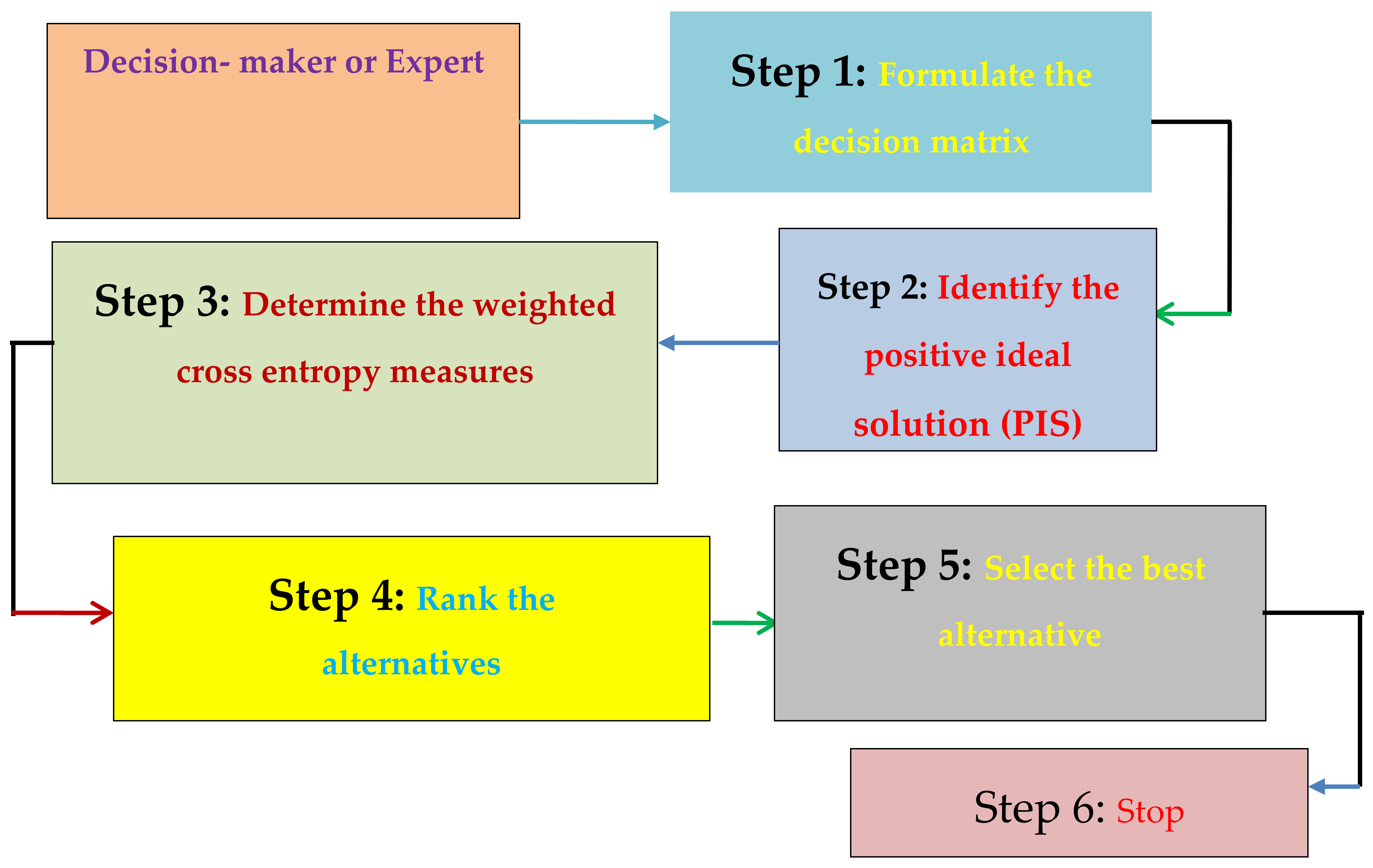
The procedure for solving MADM problems in a bipolar neutrosophic environment is presented in the following steps:

Step 1. The rating of the performance value of alternative B_i (i = 1, 2, …, m) with respect to the predefined attribute C_j (j = 1, 2, …, n) can be expressed in terms of bipolar neutrosophic information as follows:

$$B_i= \{C_j, <T_{B_i}^{+}(C_j),\hspace{0.17em}{I}_{B_i}^{+}(C_j),\hspace{0.17em}{F}_{B_i}^{+}(C_j),\hspace{0.17em}{T}_{B_i}^{-}(C_j),\hspace{0.17em}{I}_{B_i}^{-}(C_j),\hspace{0.17em}{F}_{B_i}^{-}(C_j)>|C_j\in C_j,j= 1, 2, \dots ,n\},$$

where 0 $\le$ $T_{B_i}^{+}(C_j)$ + $I_{B_i}^{+}(C_j)$ + $F_{B_i}^{+}(C_j)$ $\le$ 3 and −3 $\le$ $T_{B_i}^{-}(C_j)$ + $I_{B_i}^{-}(C_j)$ + $F_{B_i}^{-}(C_j)$ $\le$ 0, i = 1, 2, …, m; j = 1, 2, …, n.

Assume that ${\tilde{d}}_{ij}$ = <$T_{ij}^{+}$, $I_{ij}^{+}$, $F_{ij}^{+}$, $T_{ij}^{-}$, $I_{ij}^{-}$, $F_{ij}^{-}$> is the bipolar neutrosophic decision matrix whose entries are the rating values of the alternatives with respect to the attributes provided by the expert or decision-maker. The bipolar neutrosophic decision matrix ${[{\tilde{d}}_{ij}]}_{m\times n}$ can be expressed as follows:

$${[{\tilde{d}}_{ij}]}_{m\times n}=\begin{array}{l}\\ \\ B_1\\ B_2\\ .\\ .\\ B_m\end{array}\begin{array}{l}\hspace{0.17em}\hspace{0.17em}\hspace{0.17em}\hspace{0.17em}{C}_1\hspace{0.17em}\hspace{0.17em}\hspace{0.17em}\hspace{0.17em}\hspace{0.17em}{C}_2\hspace{0.17em}\hspace{0.17em}\dots \hspace{0.17em}\hspace{0.17em}{C}_n\\ \left(\begin{array}{l}\hspace{0.17em}\hspace{0.17em}\hspace{0.17em}\\ d_{11}\hspace{0.17em}\hspace{0.17em}\hspace{0.17em}\hspace{0.17em}\hspace{0.17em}{d}_{12}\hspace{0.17em}\hspace{0.17em}\dots \hspace{0.17em}\hspace{0.17em}{d}_{1n}\\ d_{21}\hspace{0.17em}\hspace{0.17em}\hspace{0.17em}\hspace{0.17em}\hspace{0.17em}{d}_{22}\hspace{0.17em}\hspace{0.17em}\dots \hspace{0.17em}\hspace{0.17em}{d}_{2n}\\ \hspace{0.17em}.\hspace{0.17em}\hspace{0.17em}\hspace{0.17em}\hspace{0.17em}\hspace{0.17em}\hspace{0.17em}\hspace{0.17em}.\hspace{0.17em}\hspace{0.17em}\hspace{0.17em}\hspace{0.17em}\dots \hspace{0.17em}\hspace{0.17em}\hspace{0.17em}.\\ \hspace{0.17em}.\hspace{0.17em}\hspace{0.17em}\hspace{0.17em}\hspace{0.17em}\hspace{0.17em}\hspace{0.17em}\hspace{0.17em}.\hspace{0.17em}\hspace{0.17em}\hspace{0.17em}\hspace{0.17em}\dots \hspace{0.17em}\hspace{0.17em}\hspace{0.17em}.\\ d_{m1}\hspace{0.17em}\hspace{0.17em}\hspace{0.17em}\hspace{0.17em}{d}_{m2}\hspace{0.17em}\hspace{0.17em}\dots \hspace{0.17em}\hspace{0.17em}{d}_{mn}\end{array}\right)\end{array}.$$

Step 2. The positive ideal solution (PIS) <p* = ($d_1^{*}$, $d_2^{*}$, ..., $d_n^{*}$)> of the bipolar neutrosophic information is obtained as follows:

$$\begin{array}{l}{p}_j^{*}\hspace{0.17em}=\hspace{0.17em}\langle T_j^{*+},I_j^{*+},F_j^{*+},T_j^{*-},I_j^{*-},F_j^{*-}\rangle \hspace{0.17em}=\hspace{0.17em}<[\{\underset{i}{Max}\hspace{0.17em}(T_{ij}^{+})|j \in H_1\}; \{\underset{i}{Min}\hspace{0.17em}(T_{ij}^{+})|j\in H_2\}],\\ [\{\underset{i}{Min}\hspace{0.17em}(I_{ij}^{+})|j \in H_1\}; \{\underset{i}{Max}\hspace{0.17em}(I_{ij}^{+})|j\in H_2\}],\hspace{0.17em}[\{\underset{i}{Min}\hspace{0.17em}\hspace{0.17em}(F_{ij}^{+})|j\in H_1\}; \{\underset{i}{Max}\hspace{0.17em}(F_{ij}^{+})|j\in H_2\}],\\ [\{\underset{i}{Min}\hspace{0.17em}(T_{ij}^{-})|j \in H_1\}; \{\underset{i}{Max}\hspace{0.17em}(T_{ij}^{-})|j\in H_2\}],\hspace{0.17em}[\{\underset{i}{Max}\hspace{0.17em}(I_{ij}^{-})|j \in H_1\}; \{\underset{i}{Min}\hspace{0.17em}(I_{ij}^{-})|j\in H_2\}],\\ [\{\underset{i}{Max}\hspace{0.17em}(F_{ij}^{-})|j \in H_1\}; \{\underset{i}{Min}\hspace{0.17em}(F_{ij}^{-})|j\in H_2\}]>, j = 1, 2, \dots ,n;\end{array}$$

where H₁ and H₂ represent benefit and cost type attributes, respectively.

Step 3. The weighted cross entropy between an alternative B_i, i = 1, 2, …, m, and the ideal alternative p^* is determined by

$$C_B{\left(B_i,p*\right)}_w={\displaystyle \sum _{i=1}^n{w}_i}\left[\begin{array}{l}\sqrt{\frac{T_{ij}^{+}+T_j^{*+}}{2}}-\left(\frac{\sqrt{T_{ij}^{+}}+\sqrt{T_j^{*+}}}{2}\right)+\sqrt{\frac{I_{ij}^{+}+I_j^{*+}}{2}}-\left(\frac{\sqrt{I_{ij}^{+}}+\sqrt{I_j^{*+}}}{2}\right)+\sqrt{\frac{[1-I_{ij}^{+}]+[1-I_j^{*+}]}{2}}-\\ \left(\frac{\sqrt{1-I_j^{+}}+\sqrt{[1-I_j^{*+}]}}{2}\right)+\sqrt{\frac{F_{ij}^{+}+F_j^{*+}}{2}}-\left(\frac{\sqrt{F_{ij}^{+}}+\sqrt{F_j^{*+}}}{2}\right)+\sqrt{\frac{-(T_{ij}^{-}+T_j^{*-})}{2}}-\\ \left(\frac{\sqrt{(-T_{ij}^{-})}+\sqrt{(-T_j^{*-})}}{2}\right)+\sqrt{\frac{-(I_{ij}^{-}+I_j^{*-})}{2}}-\left(\frac{\sqrt{(-I_{ij}^{-})}+\sqrt{(-I_j^{*-})}}{2}\right)+\sqrt{\frac{[1+I_{ij}^{-}]+[1+I_j^{*-}]}{2}}\\ -\left(\frac{\sqrt{1+I_{ij}^{-}}+\sqrt{[1+I_j^{*-}]}}{2}\right)+\sqrt{\frac{-(F_{ij}^{-}+F_j^{*-})}{2}}-\left(\frac{\sqrt{(-F_{ij}^{-})}+\sqrt{(-F_j^{*-})}}{2}\right)\end{array}\right].$$

(5)

Step 4. A smaller value of C_B(B_i, p*)_w, i = 1, 2, ..., m represents that an alternative B_i, i = 1, 2, …, m is closer to the PIS p*. Therefore, the alternative with the smallest weighted cross entropy measure is the best alternative.

5.2. MADM Strategy Based on Weighted Cross Entropy Measures of IBNSs

The steps for solving MADM problems with interval bipolar neutrosophic information are presented as follows.

Step 1. In an interval bipolar neutrosophic environment, the rating of the performance value of alternative B_i (i = 1, 2, …, m) with respect to the predefined attribute C_j (j = 1, 2, …, n) can be represented as follows:

$$\begin{array}{l}{B}_i= \{C_j, <[\inf T_{B_i}^{+}(C_j), \sup T_{B_i}^{+}(C_j)],\hspace{0.17em}[\inf I_{B_i}^{+}(C_j),\hspace{0.17em}\sup I_{B_i}^{+}(C_j)],\hspace{0.17em}[\inf F_{B_i}^{+}(C_j), \sup F_{B_i}^{+}(C_j)],\hfill \\ [\inf T_{B_i}^{-}(C_j),\hspace{0.17em}\sup T_{B_i}^{-}(C_j)],\hspace{0.17em}[\inf I_{B_i}^{-}(C_j), \sup I_{B_i}^{-}(C_j)],\hspace{0.17em}[\inf F_{B_i}^{-}(C_j), \sup F_{B_i}^{-}(C_j)]>|C_j\in C_j,\hfill \\ j= 1, 2, \dots ,n\}\hfill \end{array}$$

where 0 $\le$ sup$T_{B_i}^{+}(C_j)$ + sup$I_{B_i}^{+}(C_j)$ + sup$F_{B_i}^{+}(C_j)$ $\le$ 3 and −3 $\le$ sup$T_{B_i}^{-}(C_j)$ + sup$I_{B_i}^{-}(C_j)$ + sup$F_{B_i}^{-}(C_j)$ $\le$ 0; j = 1, 2, …, n. Let ${\tilde{g}}_{ij}$ = <[${}^{L}T{}_{ij}^{+}$, ${}^{U}T{}_{ij}^{+}$], [${}^{L}I{}_{ij}^{+}$, ${}^{U}I{}_{ij}^{+}$], [${}^{L}F{}_{ij}^{+}$, ${}^{U}F{}_{ij}^{+}$], [${}^{L}T{}_{ij}^{-}$, ${}^{U}T{}_{ij}^{-}$], [${}^{L}I{}_{ij}^{-}$, ${}^{U}I{}_{ij}^{-}$], [${}^{L}F{}_{ij}^{-}$, ${}^{U}F{}_{ij}^{-}$]> be the bipolar neutrosophic decision matrix whose entries are the rating values of the alternatives with respect to the attributes provided by the expert or decision-maker. The interval bipolar neutrosophic decision matrix ${[{\tilde{g}}_{ij}]}_{m\times n}$ can be presented as follows:

$${[{\tilde{g}}_{ij}]}_{m\times n}=\begin{array}{l}\\ \\ B_1\\ B_2\\ .\\ .\\ B_m\end{array}\begin{array}{l}\hspace{0.17em}\hspace{0.17em}\hspace{0.17em}{C}_1\hspace{0.17em}\hspace{0.17em}\hspace{0.17em}{C}_2\hspace{0.17em}\hspace{0.17em}\dots \hspace{0.17em}\hspace{0.17em}{C}_n\\ \left(\begin{array}{l}\hspace{0.17em}\hspace{0.17em}\hspace{0.17em}\\ g_{11}\hspace{0.17em}\hspace{0.17em}\hspace{0.17em}{g}_{12}\hspace{0.17em}\hspace{0.17em}\dots \hspace{0.17em}\hspace{0.17em}{g}_{1n}\\ g_{21}\hspace{0.17em}\hspace{0.17em}\hspace{0.17em}{g}_{22}\hspace{0.17em}\hspace{0.17em}\dots \hspace{0.17em}\hspace{0.17em}{g}_{2n}\\ \hspace{0.17em}.\hspace{0.17em}\hspace{0.17em}\hspace{0.17em}\hspace{0.17em}\hspace{0.17em}.\hspace{0.17em}\hspace{0.17em}\hspace{0.17em}\hspace{0.17em}\dots \hspace{0.17em}\hspace{0.17em}\hspace{0.17em}.\\ \hspace{0.17em}.\hspace{0.17em}\hspace{0.17em}\hspace{0.17em}\hspace{0.17em}\hspace{0.17em}.\hspace{0.17em}\hspace{0.17em}\hspace{0.17em}\hspace{0.17em}\dots \hspace{0.17em}\hspace{0.17em}\hspace{0.17em}.\\ g_{m1}\hspace{0.17em}\hspace{0.17em}{g}_{m2}\hspace{0.17em}\hspace{0.17em}\dots \hspace{0.17em}\hspace{0.17em}{g}_{mn}\end{array}\right)\end{array}.$$

Step 2. The PIS <q* = ($g_1^{*}$, $g_2^{*}$, ..., $g_n^{*}$)> of the interval bipolar neutrosophic information is obtained as follows:

$$\begin{array}{l}{q}_j^{*}\hspace{0.17em}=\hspace{0.17em}<[{}^{L}T{}_{ij}^{*+},\hspace{0.17em}{}^{U}T{}_{ij}^{*+}],\hspace{0.17em}[{}^{L}I{}_{ij}^{*+},\hspace{0.17em}{}^{U}I{}_{ij}^{*+}],\hspace{0.17em}[{}^{L}F{}_{ij}^{*+},\hspace{0.17em}{}^{U}F{}_{ij}^{*+}],\hspace{0.17em}[{}^{L}T{}_{ij}^{*-},\hspace{0.17em}{}^{U}T{}_{ij}^{*-}],\hspace{0.17em}[{}^{L}I{}_{ij}^{*-},\hspace{0.17em}{}^{U}I{}_{ij}^{*-}],\hspace{0.17em}[{}^{L}F{}_{ij}^{*-},\hspace{0.17em}{}^{U}F{}_{ij}^{*-}]>,\\ \hspace{0.17em}\hspace{0.17em}\hspace{0.17em}\hspace{0.17em}=\hspace{0.17em}<[\{\underset{i}{Max}\hspace{0.17em}({}^{L}T{}_{ij}^{+})|j\in H_1\};\hspace{0.17em}\{\underset{i}{Min}\hspace{0.17em}({}^{L}T{}_{ij}^{+})|j\in H_2\},\hspace{0.17em}\{\underset{i}{Max}\hspace{0.17em}({}^{U}T{}_{ij}^{+})|j\in H_1\};\hspace{0.17em}\{\underset{i}{Min}\hspace{0.17em}({}^{U}T{}_{ij}^{+})|j\in H_2\}],\\ \hspace{0.17em}\hspace{0.17em}\hspace{0.17em}\hspace{0.17em}\hspace{0.17em}\hspace{0.17em}\hspace{0.17em}\hspace{0.17em}\hspace{0.17em}[\{\underset{i}{Min}\hspace{0.17em}({}^{L}I{}_{ij}^{+})|j\in H_1\};\hspace{0.17em}\{\underset{i}{Max}\hspace{0.17em}({}^{L}I{}_{ij}^{+})|j\in H_2\},\hspace{0.17em}\{\underset{i}{Min}\hspace{0.17em}({}^{U}I{}_{ij}^{+})|j\in H_1\};\hspace{0.17em}\{\underset{i}{Max}\hspace{0.17em}({}^{U}I{}_{ij}^{+})|j\in H_2\}],\\ \hspace{0.17em}\hspace{0.17em}\hspace{0.17em}\hspace{0.17em}\hspace{0.17em}\hspace{0.17em}\hspace{0.17em}\hspace{0.17em}\hspace{0.17em}[\{\underset{i}{Min}\hspace{0.17em}({}^{L}F{}_{ij}^{+})|j\in H_1\};\hspace{0.17em}\{\underset{i}{Max}\hspace{0.17em}({}^{L}F{}_{ij}^{+})|j\in H_2\},\hspace{0.17em}\{\underset{i}{Min}\hspace{0.17em}({}^{U}F{}_{ij}^{+})|j\in H_1\};\hspace{0.17em}\{\underset{i}{Max}\hspace{0.17em}({}^{U}F{}_{ij}^{+})|j\in H_2\}],\\ \hspace{0.17em}\hspace{0.17em}\hspace{0.17em}\hspace{0.17em}\hspace{0.17em}\hspace{0.17em}\hspace{0.17em}\hspace{0.17em}\hspace{0.17em}[\{\underset{i}{Min}\hspace{0.17em}({}^{L}T{}_{ij}^{-})|j\in H_1\};\hspace{0.17em}\{\underset{i}{Max}\hspace{0.17em}({}^{L}T{}_{ij}^{-})|j\in H_2\},\hspace{0.17em}\{\underset{i}{Min}\hspace{0.17em}({}^{U}T{}_{ij}^{-})|j\in H_1\};\hspace{0.17em}\{\underset{i}{Max}\hspace{0.17em}({}^{U}T{}_{ij}^{-})|j\in H_2\}],\\ \hspace{0.17em}\hspace{0.17em}\hspace{0.17em}\hspace{0.17em}\hspace{0.17em}\hspace{0.17em}\hspace{0.17em}\hspace{0.17em}\hspace{0.17em}[\{\underset{i}{Max}\hspace{0.17em}({}^{L}I{}_{ij}^{-})|j\in H_1\};\hspace{0.17em}\{\underset{i}{Min}\hspace{0.17em}({}^{L}I{}_{ij}^{-})|j\in H_2\},\hspace{0.17em}\{\underset{i}{Max}\hspace{0.17em}({}^{U}I{}_{ij}^{-})|j\in H_1\};\hspace{0.17em}\{\underset{i}{Min}\hspace{0.17em}({}^{U}I{}_{ij}^{-})|j\in H_2\}],\\ \hspace{0.17em}\hspace{0.17em}\hspace{0.17em}\hspace{0.17em}\hspace{0.17em}\hspace{0.17em}\hspace{0.17em}\hspace{0.17em}\hspace{0.17em}[\{\underset{i}{Max}\hspace{0.17em}({}^{L}F{}_{ij}^{-})|j\in H_1\};\hspace{0.17em}\{\underset{i}{Min}\hspace{0.17em}({}^{L}F{}_{ij}^{-})|j\in H_2\},\hspace{0.17em}\{\underset{i}{Max}\hspace{0.17em}({}^{U}F{}_{ij}^{-})|j\in H_1\};\hspace{0.17em}\{\underset{i}{Min}\hspace{0.17em}({}^{U}F{}_{ij}^{-})|j\in H_2\}]>,\\ \hspace{0.17em}\hspace{0.17em}\hspace{0.17em}\hspace{0.17em}\hspace{0.17em}\hspace{0.17em}\hspace{0.17em}\hspace{0.17em} j = 1, 2, \dots ,n\end{array}$$

where H₁ and H₂ stand for benefit and cost type attributes, respectively.

Step 3. The weighted cross entropy between an alternative B_i, i = 1, 2, …, m, and the ideal alternative q* under an interval bipolar neutrosophic setting is computed as follows:

$$C_{IB}{\left(B_i,q*\right)}_w=\frac{1}{2}\hspace{0.17em}\times \hspace{0.17em}{\displaystyle \sum _{i=1}^n{w}_i}\left[\begin{array}{l}\sqrt{\frac{{}^{L}T{}_{ij}^{+}+{}^{L}T{}_j^{*+}}{2}}-\left(\frac{\sqrt{{}^{L}T{}_{ij}^{+}}+\sqrt{{}^{L}T{}_j^{*+}}}{2}\right)+\sqrt{\frac{{}^{U}T{}_{ij}^{+}+{}^{U}T{}_j^{*+}}{2}}-\left(\frac{\sqrt{{}^{U}T{}_{ij}^{+}}+\sqrt{{}^{U}T{}_j^{*+}}}{2}\right)+\sqrt{\frac{{}^{L}I{}_{ij}^{+}+{}^{L}I{}_j^{*+}}{2}}-\left(\frac{\sqrt{{}^{L}I{}_{ij}^{+}}+\sqrt{{}^{L}I{}_j^{*+}}}{2}\right)+\\ \sqrt{\frac{[1-{}^{L}I{}_{ij}^{+}]+[1-{}^{L}I{}_j^{*+}]}{2}}-\left(\frac{\sqrt{1-{}^{L}I{}_j^{+}}+\sqrt{[1-{}^{L}I{}_j^{*+}]}}{2}\right)+\sqrt{\frac{{}^{U}I{}_{ij}^{+}+{}^{U}I{}_j^{*+}}{2}}-\left(\frac{\sqrt{{}^{U}I{}_{ij}^{+}}+\sqrt{{}^{U}I{}_j^{*+}}}{2}\right)+\sqrt{\frac{[1-{}^{U}I{}_{ij}^{+}]+[1-{}^{U}I{}_j^{*+}]}{2}}-\\ \left(\frac{\sqrt{1-{}^{U}I{}_j^{+}}+\sqrt{[1-{}^{U}I{}_j^{*+}]}}{2}\right)+\sqrt{\frac{{}^{L}F{}_{ij}^{+}+{}^{L}F{}_j^{*+}}{2}}-\left(\frac{\sqrt{{}^{L}F{}_{ij}^{+}}+\sqrt{{}^{L}F{}_j^{*+}}}{2}\right)+\sqrt{\frac{{}^{U}F{}_{ij}^{+}+{}^{U}F{}_j^{*+}}{2}}-\left(\frac{\sqrt{{}^{U}F{}_{ij}^{+}}+\sqrt{{}^{U}F{}_j^{*+}}}{2}\right)+\sqrt{\frac{-({}^{L}T{}_{ij}^{-}+{}^{L}T{}_j^{*-})}{2}}-\\ \left(\frac{\sqrt{(-{}^{L}T{}_{ij}^{-})}+\sqrt{(-{}^{L}T{}_j^{*-})}}{2}\right)+\sqrt{\frac{-({}^{U}T{}_{ij}^{-}+{}^{U}T{}_j^{*-})}{2}}-\left(\frac{\sqrt{(-{}^{U}T{}_{ij}^{-})}+\sqrt{(-{}^{U}T{}_j^{*-})}}{2}\right)+\sqrt{\frac{-({}^{L}I{}_{ij}^{-}+{}^{L}I{}_j^{*-})}{2}}-\left(\frac{\sqrt{(-{}^{L}I{}_{ij}^{-})}+\sqrt{(-{}^{L}I{}_j^{*-})}}{2}\right)+\\ \sqrt{\frac{-({}^{U}I{}_{ij}^{-}+{}^{U}I{}_j^{*-})}{2}}-\left(\frac{\sqrt{(-{}^{U}I{}_{ij}^{-})}+\sqrt{(-{}^{U}I{}_j^{*-})}}{2}\right)+\sqrt{\frac{[1+{}^{L}I{}_{ij}^{-}]+[1+{}^{L}I{}_j^{*-}]}{2}}-\left(\frac{\sqrt{1+{}^{L}I{}_{ij}^{-}}+\sqrt{[1+{}^{L}I{}_j^{*-}]}}{2}\right)+\sqrt{\frac{[1+{}^{U}I{}_{ij}^{-}]+[1+{}^{U}I{}_j^{*-}]}{2}}-\\ \left(\frac{\sqrt{1+{}^{U}I{}_{ij}^{-}}+\sqrt{[1+{}^{U}I{}_j^{*-}]}}{2}\right)+\sqrt{\frac{-({}^{L}F{}_{ij}^{-}+{}^{L}F{}_j^{*-})}{2}}-\left(\frac{\sqrt{(-{}^{L}F{}_{ij}^{-})}+\sqrt{(-{}^{L}F{}_j^{*-})}}{2}\right)+\sqrt{\frac{-({}^{U}F{}_{ij}^{-}+{}^{U}F{}_j^{*-})}{2}}-\left(\frac{\sqrt{(-{}^{U}F{}_{ij}^{-})}+\sqrt{(-{}^{U}F{}_j^{*-})}}{2}\right)\end{array}\right].$$

(6)

Step 4. A smaller value of C_IB(B_i, p*)_w, i = 1, 2, ..., m indicates that an alternative B_i, i = 1, 2, …, m is closer to the PIS q*. Hence, the alternative with the smallest weighted cross entropy measure will be identified as the best alternative.

A conceptual model of the proposed strategy is shown in Figure 1.

6. Illustrative Example

In this section we solve two numerical MADM problems and a comparison with other existing strategies is presented to verify the applicability and effectiveness of the proposed strategies in bipolar neutrosophic and interval bipolar neutrosophic environments.

6.1. Car Selection Problem with Bipolar Neutrosophic Information

Consider the problem discussed in [81,86,87,88] where a buyer wants to purchase a car based on some predefined attributes. Suppose that four types of cars (alternatives) B_i, (i = 1, 2, 3, 4) are available in the market. Four attributes are taken into consideration in the decision-making environment, namely, Fuel economy (C₁), Aerod (C₂), Comfort (C₃), Safety (C₄), to select the most desirable car. Assume that the weight vector for the four attributes is known and given by w = (w₁, w₂, w₃, w₄) = (0.5, 0.25, 0.125, 0.125). Therefore, the bipolar neutrosophic decision matrix ${\langle d_{ij}\rangle }_{4\times 4}$ can be obtained as given below.

The bipolar neutrosophic decision matrix ${[{\tilde{d}}_{ij}]}_{4\times 4}$ =

	C1	C2	C3	C4
B1	<0.5, 0.7, 0.2, −0.7, −0.3, −0.6>	<0.4, 0.4, 0.5, −0.7, −0.8, −0.4>	<0.7, 0.7, 0.5, −0.8, −0.7, −0.6>	<0.1, 0.5, 0.7, −0.5, −0.2, −0.8>
B2	<0.9, 0.7, 0.5, −0.7, −0.7, −0.1>	<0.7, 0.6, 0.8, −0.7, −0.5, −0.1>	<0.9, 0.4, 0.6, −0.1, −0.7, −0.5>	<0.5, 0.2, 0.7, −0.5, −0.1, −0.9>
B3	<0.3, 0.4, 0.2, −0.6, −0.3, −0.7>	<0.2, 0.2, 0.2, −0.4, −0.7, −0.4>	<0.9, 0.5, 0.5, −0.6, −0.5, −0.2>	<0.7, 0.5, 0.3, −0.4, −0.2, −0.2>
B4	<0.9, 0.7, 0.2, −0.8, −0.6, −0.1>	<0.3, 0.5, 0.2, −0.5, −0.5, −0.2>	<0.5, 0.4, 0.5, −0.1, −0.7, −0.2>	<0.2, 0.4, 0.8, −0.5, −0.5, −0.6>

The positive ideal bipolar neutrosophic solutions are computed from ${[{\tilde{d}}_{ij}]}_{4\times 4}$ as follows:

p* = [<0.9, 0.4, 0.2, −0.8, −0.3, −0.1>, <0.7, 0.2, 0.2, −0.7, −0.5, −0.1>,
<0.9, 0.4, 0.5, −0.8, −0.5, −0.2>, <0.7, 0.2, 0.3, −0.5, −0.1, −0.2>].

Using Equation (5), the weighted cross entropy measure C_B(B_i, p*)_w is obtained as follows:

C_B(B₁, p*)_w = 0.0734, C_B(B₂, p*)_w = 0.0688, C_B(B₃, p*)_w = 0.0642, C_B(B₄, p*)_w = 0.0516.

(7)

According to the weighted cross entropy measure C_B(B_i, p*)_w, the order of the four alternatives is B₄ $\prec$ B₃ $\prec$ B₂ $\prec$ B₁; therefore, B₄ is the best car.

We compare our obtained result with the results of other existing strategies (see

Table 1. The results of the car selection problem obtained from different methods.

Methods	Ranking Results	Best Option
The proposed weighted cross entropy measure	B4$\prec$B3$\prec$B2$\prec$B1	B4
Dey et al.’s TOPSIS strategy [87]	B1$\prec$B3$\prec$B2$\prec$B4	B4
Deli et al.’s strategy [81]	B1$\prec$B2$\prec$B4$\prec$B3	B3
Projection measure [88]	B3$\prec$B4$\prec$B1$\prec$B2	B2
Bidirectional projection measure [88]	B2$\prec$B1$\prec$B4$\prec$B3	B3
Hybrid projection measure [88] with $\rho$ = 0.25	B2$\prec$B1$\prec$B3$\prec$B4	B4
Hybrid projection measure [88] with $\rho$ = 0.50	B3$\prec$B2$\prec$B1$\prec$B4	B4
Hybrid projection measure [88] with $\rho$ = 0.75	B1$\prec$B3$\prec$B4$\prec$B2	B2
Hybrid projection measure [88] with $\rho$ = 0.90	B3$\prec$B4$\prec$B2$\prec$B1	B1
Hybrid similarity measure [88] with $\rho$ = 0.25	B2$\prec$B4$\prec$B1$\prec$B3	B3
Hybrid similarity measure [88] with $\rho$ = 0.30	B2$\prec$B4$\prec$B1$\prec$B3	B3
Hybrid similarity measure [88] with $\rho$ = 0.60	B2$\prec$B4$\prec$B1$\prec$B3	B3
Hybrid similarity measure [88] with $\rho$ = 0.90	B2$\prec$B4$\prec$B3$\prec$B1	B1

), where the known weight of the attributes is given by w = (w₁, w₂, w₃, w₄) = (0.5, 0.25, 0.125, 0.125). It is to be noted that the ranking results obtained from the other existing strategies are different from the result of the proposed strategies in some cases. The reason is that the different authors adopted different decision-making strategies and thereby obtained different ranking results. However, the proposed strategies are simple and straightforward and can effectively solve decision-making problems with bipolar neutrosophic information.

6.2. Interval Bipolar Neutrosophic MADM Investment Problem

Consider an interval bipolar neutrosophic MADM problem studied in [91] with four possible alternatives with the aim to invest a sum of money in the best choice. The four alternatives are:

• > a food company (B₁),
• > a car company (B₂),
• > an arms company (B₃), and
• > a computer company (B₄).

The investment company selects the best option based on three predefined attributes, namely, growth analysis (C₁), risk analysis (C₂), and environment analysis (C₃). We consider C₁ and C₂ to be benefit type attributes and C₃ to be a cost type attribute based on Ye [93]. Assume that the weight vector [91] of C₁, C₂, and C₃ is given by w = (w₁, w₂, w₃) = (0.35, 0.25, 0.4). The interval bipolar neutrosophic decision matrix ${[{\tilde{g}}_{ij}]}_{4\times 3}$ presented by the decision-maker or expert is as follows.

Interval bipolar neutrosophic decision matrix ${[{\tilde{g}}_{ij}]}_{4\times 3}$ =

$$C_1$$

$$\left(\begin{array}{l}{B}_1\hspace{0.17em}\hspace{0.17em}\hspace{0.17em}\hspace{0.17em}\hspace{0.17em}\left[[0.4,\hspace{0.17em}0.5],\hspace{0.17em}[0.2,\hspace{0.17em}0.3],\hspace{0.17em}[0.3,\hspace{0.17em}0.4],[-0.3,\hspace{0.17em}-0.2],\hspace{0.17em}[-0.4,\hspace{0.17em}-0.3],\hspace{0.17em}[-0.5,-\hspace{0.17em}0.4]\right]\\ B_2\hspace{0.17em}\hspace{0.17em}\hspace{0.17em}\hspace{0.17em}\hspace{0.17em}\left[[0.6,\hspace{0.17em}0.7],\hspace{0.17em}[0.1,\hspace{0.17em}0.2],\hspace{0.17em}[0.2,\hspace{0.17em}0.3],[-0.2,\hspace{0.17em}-0.1],\hspace{0.17em}[-0.3,\hspace{0.17em}-0.2],\hspace{0.17em}[-0.7,-\hspace{0.17em}0.6]\right]\\ B_3\hspace{0.17em}\hspace{0.17em}\hspace{0.17em}\hspace{0.17em}\hspace{0.17em}\left[[0.3,\hspace{0.17em}0.6],\hspace{0.17em}[0.2,\hspace{0.17em}0.3],\hspace{0.17em}[0.3,\hspace{0.17em}0.4],[-0.3,\hspace{0.17em}-0.2],\hspace{0.17em}[-0.4,\hspace{0.17em}-0.3],\hspace{0.17em}[-0.6,-\hspace{0.17em}0.3]\right]\\ B_4\hspace{0.17em}\hspace{0.17em}\hspace{0.17em}\hspace{0.17em}\hspace{0.17em}\left[[0.7,\hspace{0.17em}0.8],\hspace{0.17em}[0.0,\hspace{0.17em}0.1],\hspace{0.17em}[0.1,\hspace{0.17em}0.2],[-0.1,\hspace{0.17em}-0.0],\hspace{0.17em}[-0.2,\hspace{0.17em}-0.1],\hspace{0.17em}[-0.8,-\hspace{0.17em}0.7]\right]\end{array}\right)$$

$$C_2$$

$$\left(\begin{array}{l}{B}_1\hspace{0.17em}\hspace{0.17em}\hspace{0.17em}\hspace{0.17em}\hspace{0.17em}\left[[0.4,\hspace{0.17em}0.6],\hspace{0.17em}[0.1,\hspace{0.17em}0.3],\hspace{0.17em}[0.2,\hspace{0.17em}0.4],[-0.3,\hspace{0.17em}-0.1],\hspace{0.17em}[-0.4,\hspace{0.17em}-0.2],\hspace{0.17em}[-0.6,-\hspace{0.17em}0.4]\right]\\ B_2\hspace{0.17em}\hspace{0.17em}\hspace{0.17em}\hspace{0.17em}\hspace{0.17em}\left[[0.6,\hspace{0.17em}0.7],\hspace{0.17em}[0.1,\hspace{0.17em}0.2],\hspace{0.17em}[0.2,\hspace{0.17em}0.3],[-0.2,\hspace{0.17em}-0.1],\hspace{0.17em}[-0.3,\hspace{0.17em}-0.2],\hspace{0.17em}[-0.7,-\hspace{0.17em}0.6]\right]\\ B_3\hspace{0.17em}\hspace{0.17em}\hspace{0.17em}\hspace{0.17em}\hspace{0.17em}\left[[0.5,\hspace{0.17em}0.6],\hspace{0.17em}[0.2,\hspace{0.17em}0.3],\hspace{0.17em}[0.3,\hspace{0.17em}0.4],[-0.3,\hspace{0.17em}-0.2],\hspace{0.17em}[-0.4,\hspace{0.17em}-0.3],\hspace{0.17em}[-0.6,-\hspace{0.17em}0.5]\right]\\ B_4\hspace{0.17em}\hspace{0.17em}\hspace{0.17em}\hspace{0.17em}\hspace{0.17em}\left[[0.6,\hspace{0.17em}0.7],\hspace{0.17em}[0.1,\hspace{0.17em}0.2],\hspace{0.17em}[0.1,\hspace{0.17em}0.3],[-0.2\hspace{0.17em}-0.1],\hspace{0.17em}[-0.3,\hspace{0.17em}-0.1],\hspace{0.17em}[-0.7,-\hspace{0.17em}0.6]\right]\end{array}\right)$$

$$C_3$$

$$\left(\begin{array}{l}{B}_1\hspace{0.17em}\hspace{0.17em}\hspace{0.17em}\hspace{0.17em}\hspace{0.17em}\left[[0.7,\hspace{0.17em}0.9],\hspace{0.17em}[0.2,\hspace{0.17em}0.3],\hspace{0.17em}[0.4,\hspace{0.17em}0.5],[-0.3,\hspace{0.17em}-0.2],\hspace{0.17em}[-0.5,\hspace{0.17em}-0.4],\hspace{0.17em}[-0.9,-\hspace{0.17em}0.7]\right]\\ B_2\hspace{0.17em}\hspace{0.17em}\hspace{0.17em}\hspace{0.17em}\hspace{0.17em}\left[[0.3,\hspace{0.17em}0.6],\hspace{0.17em}[0.3,\hspace{0.17em}0.5],\hspace{0.17em}[0.8,\hspace{0.17em}0.9],[-0.5,\hspace{0.17em}-0.3],\hspace{0.17em}[-0.9,\hspace{0.17em}-0.8],\hspace{0.17em}[-0.6,-\hspace{0.17em}0.3]\right]\\ B_3\hspace{0.17em}\hspace{0.17em}\hspace{0.17em}\hspace{0.17em}\hspace{0.17em}\left[[0.4,\hspace{0.17em}0.5],\hspace{0.17em}[0.2,\hspace{0.17em}0.4],\hspace{0.17em}[0.7,\hspace{0.17em}0.9],[-0.4,\hspace{0.17em}-0.2],\hspace{0.17em}[-0.9,\hspace{0.17em}-0.7],\hspace{0.17em}[-0.5,-\hspace{0.17em}0.4]\right]\\ B_4\hspace{0.17em}\hspace{0.17em}\hspace{0.17em}\hspace{0.17em}\hspace{0.17em}\left[[0.6,\hspace{0.17em}0.7],\hspace{0.17em}[0.3,\hspace{0.17em}0.4],\hspace{0.17em}[0.8,\hspace{0.17em}0.9],[-0.4,\hspace{0.17em}-0.3],\hspace{0.17em}[-0.9,\hspace{0.17em}-0.8],\hspace{0.17em}[-0.7,-\hspace{0.17em}0.6]\right]\end{array}\right)$$

From the matrix ${[{\tilde{g}}_{ij}]}_{4\times 3}$, we determine the positive ideal interval bipolar neutrosophic solution (q*) by using Equation (6) as follows:

q* = <[0.7, 0.8], [0.0, 0.1], [0.1, 0.2], [−0.3, −0.2], [−0.2, −0.1], [−0.5, −0.3]>;
<[0.6, 0.7], [0.1, 0.2], [0.1, 0.3], [−0.3, −0.2], [−0.3, −0.1], [−0.6, −0.4]>;
<[0.3, 0.5], [0.3, 0.5], [0.8, 0.9], [−0.3, −0.2], [−0.9, −0.8], [−0.9, −0.7]>.

The weighted cross entropy between an alternative B_i, i = 1, 2, …, m, and the ideal alternative q* can be obtained as given below:

C_IB(B₁, q*)_w = 0.0606, C_IB(B₂, q*)_w = 0.0286, C_IB(B₃, q*)_w = 0.0426, C_IB(B₄, q*)_w = 0.0423.

On the basis of the weighted cross entropy measure C_IB(B_i, q*)_w, the order of the four alternatives is B₂ $\prec$ B₄ $\prec$ B₃ $\prec$ B₁; therefore, B₂ is the best choice.

Next, the comparison of the results obtained from different methods is presented in

Table 2. The results of the investment problem obtained from different methods.

Methods	Ranking Results	Best Option
The proposed weighted cross entropy measure	B2$\prec$B4$\prec$B3$\prec$B1	B2
Mahmood et al.’s strategy [91]	B2$\prec$B3$\prec$B1$\prec$B4	B4

where the weight vector of the attribute is given by w = (w₁, w₂, w₃) = (0.35, 0.25, 0.4). We observe that B₂ is the best option obtained using the proposed method and B₄ is the best option obtained using the method of Mahmood et al. [91]. The reason for this may be that we use the interval bipolar neutrosophic cross entropy method whereas Mahmood et al. [91] derived the most desirable alternative based on a weighted arithmetic average operator in an interval bipolar neutrosophic setting.

7. Conclusions

In this paper we defined cross entropy and weighted cross entropy measures for bipolar neutrosophic sets and proved their basic properties. We also extended the proposed concept to the interval bipolar neutrosophic environment and proved its basic properties. The proposed cross entropy measures were then employed to develop two new multi-attribute decision-making strategies. Two illustrative numerical examples were solved and comparisons with existing strategies were provided to demonstrate the feasibility, applicability, and efficiency of the proposed strategies. We hope that the proposed cross entropy measures can be effective in dealing with group decision-making, data analysis, medical diagnosis, selection of a suitable company to build power plants [94], teacher selection [95], quality brick selection [96], weaver selection [97,98], etc. In future, the cross entropy measures can be extended to other neutrosophic hybrid environments, such as bipolar neutrosophic soft expert sets, bipolar neutrosophic refined sets, etc.

References

- Shannon, C.E.; Weaver, W. The Mathematical Theory of Communications; The University of Illinois Press: Urbana, IL, USA, 1949. [Google Scholar]
- Shannon, C.E. A mathematical theory of communications. Bell Syst. Tech. J. 1948, 27, 379–423. [Google Scholar] [CrossRef]
- Criado, F.; Gachechiladze, T. Entropy of fuzzy events. Fuzzy Sets Syst. 1997, 88, 99–106. [Google Scholar] [CrossRef]
- Herencia, J.; Lamta, M. Entropy measure associated with fuzzy basic probability assignment. In Proceedings of the IEEE International Conference on Fuzzy Systems, Barcelona, Spain, 5 July 1997; Volume 2, pp. 863–868. [Google Scholar]
- Rudas, I.; Kaynak, M. Entropy basedoperations on fuzzy sets. IEEE Trans. Fuzzy Syst. 1998, 6, 33–39. [Google Scholar] [CrossRef]
- Zadeh, L.A. Probality measures of fuzzy events. J. Math. Anal. Appl. 1968, 23, 421–427. [Google Scholar] [CrossRef]
- Luca, A.D.; Termini, S. A definition of non-probabilistic entropy in the setting of fuzzy set theory. Inf. Control 1972, 20, 301–312. [Google Scholar] [CrossRef]
- Sander, W. On measure of fuzziness. Fuzzy Sets Syst. 1989, 29, 49–55. [Google Scholar] [CrossRef]
- Xie, W.; Bedrosian, S. An information measure for fuzzy sets. IEEE Trans. Syst. Man Cybern. 1984, 14, 151–156. [Google Scholar] [CrossRef]
- Pal, N.; Pal, S. Higher order fuzzy entropy and hybridentropy of a fuzzy set. Inf. Sci. 1992, 61, 211–221. [Google Scholar] [CrossRef]
- Kaufmann, A.; Gupta, M. Introduction of Fuzzy Arithmetic: Theory and Applications; Van Nostrand Reinhold Co.: New York, NY, USA, 1985. [Google Scholar]
- Yager, R. On the measure of fuzziness and negation. Part I: Membership in the unit interval. Int. J. Gen. Syst. 1979, 5, 221–229. [Google Scholar] [CrossRef]
- Yager, R. On the measure of fuzziness and negation. Part II: Lattice. Inf. Control 1980, 44, 236–260. [Google Scholar] [CrossRef]
- Kosko, B. Fuzzy entropy and conditioning. Inf. Sci. 1986, 40, 165–174. [Google Scholar] [CrossRef]
- Kosko, B. Concepts of fuzzy information measure on continuous domains. Int. J. Gen. Syst. 1990, 17, 211–240. [Google Scholar] [CrossRef]
- Prakash, O.; Sharma, P.K.; Mahajan, R. New measures of weighted fuzzy entropy and their applications for the study of maximum weighted fuzzy entropy principle. Inf. Sci. 2008, 178, 2389–2395. [Google Scholar] [CrossRef]
- Burillo, P.; Bustince, H. Entropy on intuitionistic fuzzy sets and on interval–valued fuzzy sets. Fuzzy Sets Syst. 1996, 78, 305–316. [Google Scholar] [CrossRef]
- Szmidt, E.; Kacprzyk, J. Entropy for intuitionistic fuzzy sets. Fuzzy Sets Syst. 2001, 118, 467–477. [Google Scholar] [CrossRef]
- Wei, C.P.; Wang, P.; Zhang, Y.Z. Entropy, similarity measure of interval–valued intuitionistic fuzzy sets and their applications. Inf. Sci. 2011, 181, 4273–4286. [Google Scholar] [CrossRef]
- Li, X.Y. Interval–valued intuitionistic fuzzy continuous cross entropy and its application in multi-attribute decision-making. Comput. Eng. Appl. 2013, 49, 234–237. [Google Scholar]
- Shang, X.G.; Jiang, W.S. A note on fuzzy information measures. Pattern Recogit. Lett. 1997, 18, 425–432. [Google Scholar] [CrossRef]
- Vlachos, I.K.; Sergiadis, G.D. Intuitionistic fuzzy information applications to pattern recognition. Pattern Recogit. Lett. 2007, 28, 197–206. [Google Scholar] [CrossRef]
- Ye, J. Fuzzy cross entropy of interval–valued intuitionistic fuzzy sets and its optimal decision-making method based on the weights of the alternatives. Expert Syst. Appl. 2011, 38, 6179–6183. [Google Scholar] [CrossRef]
- Xia, M.M.; Xu, Z.S. Entropy/cross entropy–based group decision making under intuitionistic fuzzy sets. Inf. Fusion 2012, 13, 31–47. [Google Scholar] [CrossRef]
- Tong, X.; Yu, L.A. A novel MADM approach based on fuzzy cross entropy with interval-valued intuitionistic fuzzy sets. Math. Probl. Eng. 2015, 2015, 1–9. [Google Scholar] [CrossRef]
- Smarandache, F. A Unifying Field of Logics. Neutrosophy: Neutrosophic Probability, Set and Logic; American Research Press: Rehoboth, DE, USA, 1998. [Google Scholar]
- Zadeh, L.A. Fuzzy sets. Inf. Control 1965, 8, 338–353. [Google Scholar] [CrossRef]
- Atanassov, K.T. Intuitionistic fuzzy sets. Fuzzy Sets Syst. 1986, 20, 87–96. [Google Scholar] [CrossRef]
- Wang, H.; Smarandache, F.; Zhang, Y.Q.; Sunderraman, R. Single valued neutrosophic sets. Multispace Multistruct. 2010, 4, 410–413. [Google Scholar]
- Pramanik, S.; Biswas, P.; Giri, B.C. Hybrid vector similarity measures and their applications to multi-attribute decision making under neutrosophic environment. Neural Comput. Appl. 2017, 28, 1163–1176. [Google Scholar] [CrossRef]
- Biswas, P.; Pramanik, S.; Giri, B.C. Entropy based grey relational analysis method for multi-attribute decision making under single valued neutrosophic assessments. Neutrosophic Sets Syst. 2014, 2, 102–110. [Google Scholar]
- Biswas, P.; Pramanik, S.; Giri, B.C. A new methodology for neutrosophic multi-attribute decision making with unknown weight information. Neutrosophic Sets Syst. 2014, 3, 42–52. [Google Scholar]
- Biswas, P.; Pramanik, S.; Giri, B.C. TOPSIS method for multi-attribute group decision-making under single valued neutrosophic environment. Neural Comput. Appl. 2015. [Google Scholar] [CrossRef]
- Biswas, P.; Pramanik, S.; Giri, B.C. Aggregation of triangular fuzzy neutrosophic set information and its application to multi-attribute decision making. Neutrosophic Sets Syst. 2016, 12, 20–40. [Google Scholar]
- Biswas, P.; Pramanik, S.; Giri, B.C. Value and ambiguity index based ranking method of single-valued trapezoidal neutrosophic numbers and its application to multi-attribute decision making. Neutrosophic Sets Syst. 2016, 12, 127–138. [Google Scholar]
- Biswas, P.; Pramanik, S.; Giri, B.C. Multi-attribute group decision making based on expected value of neutrosophic trapezoidal numbers. In New Trends in Neutrosophic Theory and Applications; Smarandache, F., Pramanik, S., Eds.; Pons Editions: Brussels, Belgium, 2017; Volume II, in press. [Google Scholar]
- Biswas, P.; Pramanik, S.; Giri, B.C. Non-linear programming approach for single-valued neutrosophic TOPSIS method. New Math. Nat. Comput. 2017, in press. [Google Scholar]
- Deli, I.; Subas, Y. A ranking method of single valued neutrosophic numbers and its applications to multi-attribute decision making problems. Int. J. Mach. Learn. Cybern. 2016. [Google Scholar] [CrossRef]
- Ji, P.; Wang, J.Q.; Zhang, H.Y. Frank prioritized Bonferroni mean operator with single-valued neutrosophic sets and its application in selecting third-party logistics providers. Neural Comput. Appl. 2016. [Google Scholar] [CrossRef]
- Kharal, A. A neutrosophic multi-criteria decision making method. New Math. Nat. Comput. 2014, 10, 143–162. [Google Scholar] [CrossRef]
- Liang, R.X.; Wang, J.Q.; Li, L. Multi-criteria group decision making method based on interdependent inputs of single valued trapezoidal neutrosophic information. Neural Comput. Appl. 2016. [Google Scholar] [CrossRef]
- Liang, R.X.; Wang, J.Q.; Zhang, H.Y. A multi-criteria decision-making method based on single-valued trapezoidal neutrosophic preference relations with complete weight information. Neural Comput. Appl. 2017. [Google Scholar] [CrossRef]
- Liu, P.; Chu, Y.; Li, Y.; Chen, Y. Some generalized neutrosophic number Hamacher aggregation operators and their application to group decision making. Int. J. Fuzzy Syst. 2014, 16, 242–255. [Google Scholar]
- Liu, P.D.; Li, H.G. Multiple attribute decision-making method based on some normal neutrosophic Bonferroni mean operators. Neural Comput. Appl. 2017, 28, 179–194. [Google Scholar] [CrossRef]
- Liu, P.; Wang, Y. Multiple attribute decision-making method based on single-valued neutrosophic normalized weighted Bonferroni mean. Neural Comput. Appl. 2014, 25, 2001–2010. [Google Scholar] [CrossRef]
- Peng, J.J.; Wang, J.Q.; Wang, J.; Zhang, H.Y.; Chen, X.H. Simplified neutrosophic sets and their applications in multi-criteria group decision-making problems. Int. J. Syst. Sci. 2016, 47, 2342–2358. [Google Scholar] [CrossRef]
- Peng, J.; Wang, J.; Zhang, H.; Chen, X. An outranking approach for multi-criteria decision-making problems with simplified neutrosophic sets. Appl. Soft Comput. 2014, 25, 336–346. [Google Scholar] [CrossRef]
- Pramanik, S.; Banerjee, D.; Giri, B.C. Multi–criteria group decision making model in neutrosophic refined set and its application. Glob. J. Eng. Sci. Res. Manag. 2016, 3, 12–18. [Google Scholar]
- Pramanik, S.; Dalapati, S.; Roy, T.K. Logistics center location selection approach based on neutrosophic multi-criteria decision making. In New Trends in Neutrosophic Theory and Applications; Smarandache, F., Pramanik, S., Eds.; Pons Asbl: Brussels, Belgium, 2016; Volume 1, pp. 161–174. ISBN 978-1-59973-498-9. [Google Scholar]
- Sahin, R.; Karabacak, M. A multi attribute decision making method based on inclusion measure for interval neutrosophic sets. Int. J. Eng. Appl. Sci. 2014, 2, 13–15. [Google Scholar]
- Sahin, R.; Kucuk, A. Subsethood measure for single valued neutrosophic sets. J. Intell. Fuzzy Syst. 2014. [Google Scholar] [CrossRef]
- Sahin, R.; Liu, P. Maximizing deviation method for neutrosophic multiple attribute decision making with incomplete weight information. Neural Comput. Appl. 2016, 27, 2017–2029. [Google Scholar] [CrossRef]
- Sodenkamp, M. Models, Strategies and Applications of Group Multiple-Criteria Decision Analysis in Complex and Uncertain Systems. Ph.D. Thesis, University of Paderborn, Paderborn, Germany, 2013. [Google Scholar]
- Ye, J. Multicriteria decision-making method using the correlation coefficient under single-valued neutrosophic environment. Int. J. Gen. Syst. 2013, 42, 386–394. [Google Scholar] [CrossRef]
- Ye, J. Another form of correlation coefficient between single valued neutrosophic sets and its multiple attribute decision making method. Neutrosophic Sets Syst. 2013, 1, 8–12. [Google Scholar]
- Ye, J. A multi criteria decision-making method using aggregation operators for simplified neutrosophic sets. J. Intell. Fuzzy Syst. 2014, 26, 2459–2466. [Google Scholar]
- Ye, J. Trapezoidal neutrosophic set and its application to multiple attribute decision-making. Neural Comput. Appl. 2015, 26, 1157–1166. [Google Scholar] [CrossRef]
- Ye, J. Bidirectional projection method for multiple attribute group decision making with neutrosophic number. Neural Comput. Appl. 2015. [Google Scholar] [CrossRef]
- Ye, J. Projection and bidirectional projection measures of single valued neutrosophic sets and their decision—Making method for mechanical design scheme. J. Exp. Theor. Artif. Intell. 2016. [Google Scholar] [CrossRef]
- Nancy, G.H. Novel single-valued neutrosophic decision making operators under Frank norm operations and its application. Int. J. Uncertain. Quant. 2016, 6, 361–375. [Google Scholar] [CrossRef]
- Nancy, G.H. Some new biparametric distance measures on single-valued neutrosophic sets with applications to pattern recognition and medical diagnosis. Information 2017, 8, 162. [Google Scholar] [CrossRef]
- Pramanik, S.; Roy, T.K. Neutrosophic game theoretic approach to Indo-Pak conflict over Jammu-Kashmir. Neutrosophic Sets Syst. 2014, 2, 82–101. [Google Scholar]
- Mondal, K.; Pramanik, S. Multi-criteria group decision making approach for teacher recruitment in higher education under simplified Neutrosophic environment. Neutrosophic Sets Syst. 2014, 6, 28–34. [Google Scholar]
- Mondal, K.; Pramanik, S. Neutrosophic decision making model of school choice. Neutrosophic Sets Syst. 2015, 7, 62–68. [Google Scholar]
- Cheng, H.D.; Guo, Y. A new neutrosophic approach to image thresholding. New Math. Nat. Comput. 2008, 4, 291–308. [Google Scholar] [CrossRef]
- Guo, Y.; Cheng, H.D. New neutrosophic approach to image segmentation. Pattern Recogit. 2009, 42, 587–595. [Google Scholar] [CrossRef]
- Guo, Y.; Sengur, A.; Ye, J. A novel image thresholding algorithm based on neutrosophic similarity score. Measurement 2014, 58, 175–186. [Google Scholar] [CrossRef]
- Ye, J. Single valued neutrosophic minimum spanning tree and its clustering method. J. Intell. Syst. 2014, 23, 311–324. [Google Scholar] [CrossRef]
- Ye, J. Clustering strategies using distance-based similarity measures of single-valued neutrosophic sets. J. Intell. Syst. 2014, 23, 379–389. [Google Scholar]
- Mondal, K.; Pramanik, S. A study on problems of Hijras in West Bengal based on neutrosophic cognitive maps. Neutrosophic Sets Syst. 2014, 5, 21–26. [Google Scholar]
- Pramanik, S.; Chakrabarti, S. A study on problems of construction workers in West Bengal based on neutrosophic cognitive maps. Int. J. Innov. Res. Sci. Eng. Technol. 2013, 2, 6387–6394. [Google Scholar]
- Majumdar, P.; Samanta, S.K. On similarity and entropy of neutrosophic sets. J. Intell. Fuzzy Syst. 2014, 26, 1245–1252. [Google Scholar]
- Ye, J. Single valued neutrosophic cross-entropy for multi criteria decision making problems. Appl. Math. Model. 2014, 38, 1170–1175. [Google Scholar] [CrossRef]
- Ye, J. Improved cross entropy measures of single valued neutrosophic sets and interval neutrosophic sets and their multi criteria decision making strategies. Cybern. Inf. Technol. 2015, 15, 13–26. [Google Scholar] [CrossRef]
- Wang, H.; Smarandache, F.; Zhang, Y.Q.; Sunderraman, R. Interval Neutrosophic Sets and Logic: Theory and Applications in Computing; Hexis: Phoenix, AZ, USA, 2005. [Google Scholar]
- Pramanik, S.; Dalapati, S.; Alam, S.; Smarandache, F.; Roy, T.K. NS-cross entropy-based MAGDM under single-valued neutrosophic set environment. Information 2018, 9, 37. [Google Scholar] [CrossRef]
- Sahin, R. Cross-entropy measure on interval neutrosophic sets and its applications in multi criteria decision making. Neural Comput. Appl. 2015. [Google Scholar] [CrossRef]
- Tian, Z.P.; Zhang, H.Y.; Wang, J.; Wang, J.Q.; Chen, X.H. Multi-criteria decision-making method based on a cross-entropy with interval neutrosophic sets. Int. J. Syst. Sci. 2015. [Google Scholar] [CrossRef]
- Hwang, C.L.; Yoon, K. Multiple Attribute Decision Making: Methods and Applications; Springer: New York, NY, USA, 1981. [Google Scholar]
- Dalapati, S.; Pramanik, S.; Alam, S.; Smarandache, S.; Roy, T.K. IN-cross entropy based magdm strategy under interval neutrosophic set environment. Neutrosophic Sets Syst. 2017, 18, 43–57. [Google Scholar] [CrossRef]
- Deli, I.; Ali, M.; Smarandache, F. Bipolar neutrosophic sets and their application based on multi-criteria decision making problems. In Proceedings of the 2015 International Conference on Advanced Mechatronic Systems (ICAMechS), Beijing, China, 22–24 August 2015; pp. 249–254. [Google Scholar]
- Zhang, W.R. Bipolar fuzzy sets. In Proceedings of the IEEE World Congress on Computational Science (FuzzIEEE), Anchorage, AK, USA, 4–9 May 1998; pp. 835–840. [Google Scholar] [CrossRef]
- Zhang, W.R. Bipolar fuzzy sets and relations: A computational framework for cognitive modeling and multiagent decision analysis. In Proceedings of the IEEE Industrial Fuzzy Control and Intelligent Systems Conference, and the NASA Joint Technology Workshop on Neural Networks and Fuzzy Logic, Fuzzy Information Processing Society Biannual Conference, San Antonio, TX, USA, 18–21 December 1994; pp. 305–309. [Google Scholar] [CrossRef]
- Deli, I.; Subas, Y.A. Multiple criteria decision making method on single valued bipolar neutrosophic set based on correlation coefficient similarity measure. In Proceedings of the International Conference on Mathematics and Mathematics Education (ICMME-2016), Elazg, Turkey, 12–14 May 2016. [Google Scholar]
- Şahin, M.; Deli, I.; Uluçay, V. Jaccard vector similarity measure of bipolar neutrosophic set based on multi-criteria decision making. In Proceedings of the International Conference on Natural Science and Engineering (ICNASE’16), Killis, Turkey, 19–20 March 2016. [Google Scholar]
- Uluçay, V.; Deli, I.; Şahin, M. Similarity measures of bipolar neutrosophic sets and their application to multiple criteria decision making. Neural Comput. Appl. 2016. [Google Scholar] [CrossRef]
- Dey, P.P.; Pramanik, S.; Giri, B.C. TOPSIS for solving multi-attribute decision making problems under bi-polar neutrosophic environment. In New Trends in Neutrosophic Theory and Applications; Smarandache, F., Pramanik, S., Eds.; Pons Asbl: Brussells, Belgium, 2016; pp. 65–77. ISBN 978-1-59973-498-9. [Google Scholar]
- Pramanik, S.; Dey, P.P.; Giri, B.C.; Smarandache, F. Bipolar neutrosophic projection based models for solving multi-attribute decision making problems. Neutrosophic Sets Syst. 2017, 15, 74–83. [Google Scholar] [CrossRef]
- Wang, L.; Zhang, H.; Wang, J. Frank Choquet Bonferroni operators of bipolar neutrosophic sets and their applications to multi-criteria decision-making problems. Int. J. Fuzzy Syst. 2017. [Google Scholar] [CrossRef]
- Pramanik, S.; Dalapati, S.; Alam, S.; Smarandache, F.; Roy, T.K. TODIM Method for Group Decision Making under Bipolar Neutrosophic Set Environment. In New Trends in Neutrosophic Theory and Applications; Smarandache, F., Pramanik, S., Eds.; Pons Editions: Brussels, Belgium, 2016; Volume II, in press. [Google Scholar]
- Mahmood, T.; Ye, J.; Khan, Q. Bipolar Interval Neutrosophic Set and Its Application in Multicriteria Decision Making. Available online: https://archive.org/details/BipolarIntervalNeutrosophicSet (accessed on 9 October 2017).
- Deli, I.; Şubaș, Y.; Smarandache, F.; Ali, M. Interval Valued Bipolar Neutrosophic Sets and Their Application in Pattern Recognition. Available online: https://www.researchgate.net/publication/289587637 (accessed on 9 October 2017).
- Ye, J. Similarity measures between interval neutrosophic sets and their applications in multicriteria decision-making. J. Intell. Fuzzy Syst. 2014, 26, 165–172. [Google Scholar] [CrossRef]
- Garg, H. Non-linear programming method for multi-criteria decision making problems under interval neutrosophic set environment. Appl. Intell. 2017, 1–15. [Google Scholar] [CrossRef]
- Pramanik, S.; Mukhopadhyaya, D. Grey relational analysis-based intuitionistic fuzzy multi-criteria group decision-making approach for teacher selection in higher education. Int. J. Comput. Appl. 2011, 34, 21–29. [Google Scholar] [CrossRef]
- Mondal, K.; Pramanik, S. Intuitionistic fuzzy multi criteria group decision making approach to quality-brick selection problem. J. Appl. Quant. Methods 2014, 9, 35–50. [Google Scholar]
- Dey, P.P.; Pramanik, S.; Giri, B.C. Multi-criteria group decision making in intuitionistic fuzzy environment based on grey relational analysis for weaver selection in Khadi institution. J. Appl. Quant. Methods 2015, 10, 1–14. [Google Scholar]
- Dey, P.P.; Pramanik, S.; Giri, B.C. An extended grey relational analysis based interval neutrosophic multi-attribute decision making for weaver selection. J. New Theory 2015, 9, 82–93. [Google Scholar]
Figure 1.
Conceptual model of the proposed strategy.