Mathematical Modeling of Rogue Waves: A Survey of Recent and Emerging Mathematical Methods and Solutions


1
Department of Cell and Molecular Biology, Uppsala University, Box 596, SE-75124 Uppsala, Sweden
2
Fjordforsk A/S, Midtun, 6894 Vangsnes, Norway
Axioms 2018, 7(2), 42; https://doi.org/10.3390/axioms7020042
Submission received: 16 May 2018
/
Revised: 6 June 2018
/
Accepted: 8 June 2018
/
Published: 20 June 2018
(This article belongs to the Special Issue Applications of Differential Geometry)
Abstract
:Anomalous waves and rogue events are closely associated with irregularities and unexpected events occurring at various levels of physics, such as in optics, in oceans and in the atmosphere. Mathematical modeling of rogue waves is a highly active field of research, which has evolved over the last few decades into a specialized part of mathematical physics. The applications of the mathematical models for rogue events is directly relevant to technology development for the prediction of rogue ocean waves and for signal processing in quantum units. In this survey, a comprehensive perspective of the most recent developments of methods for representing rogue waves is given, along with discussion of the devised forms and solutions. The standard nonlinear Schrödinger equation, the Hirota equation, the MMT equation and other models are discussed and their properties highlighted. This survey shows that the most recent advancement in modeling rogue waves give models that can be used to establish methods for the prediction of rogue waves in open seas, which is important for the safety and activity of marine vessels and installations. The study further puts emphasis on the difference between the methods and how the resulting models form the basis for representing rogue waves in various forms, solitary or with a wave background. This review has also a pedagogic component directed towards students and interested non-experts and forms a complete survey of the most conventional and emerging methods published until recently.
1. Introduction
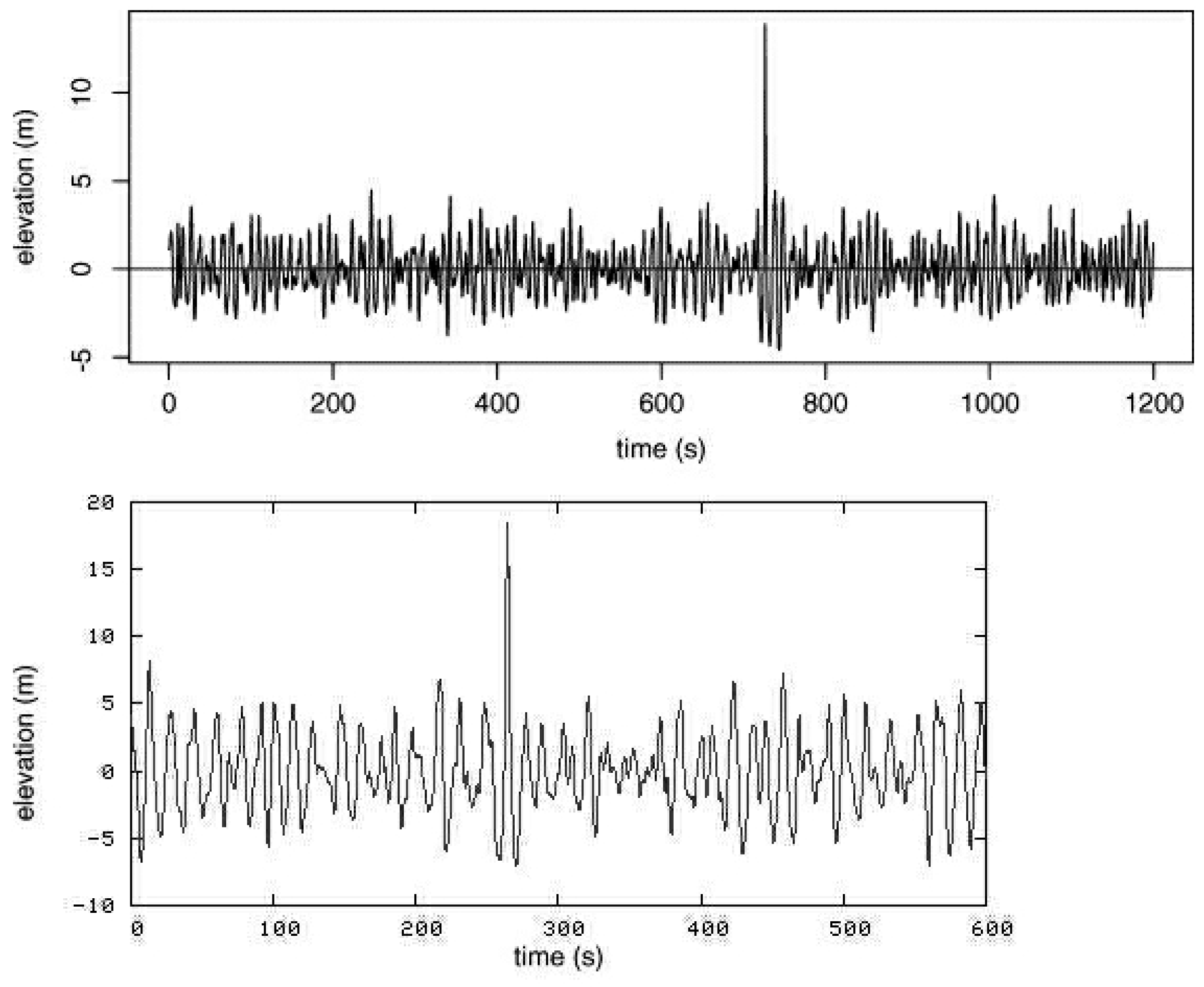
Anomalous waves, or “rogue waves”, represent a rare phenomenon at sea, which occurs on multiple occasions yearly [1,2] and causes millions of dollars of loss of cargo and loss of lives annually [3]. Rogue waves are abnormally elevated waves, with a height 2–3× that of the normal average wave and unusually having steep shapes [4,5]. Rogue waves were recorded for the first time in 1995 during a winter storm in the North Sea, when the “New Years Wave” hit the Draupner platform with a wave height of 27 m and 2.25× the average wave height [4]. The laser installation on the deck, which regularly records the elevation of the platform over the sea bed, registered the solitary giant wave with its elevation 15.4 m above and 11.6 m below the zero-level [4]. The shape of the wave was symmetrical (Figure 1) with a Gaussian bell shape and with a particularly narrow wavelength. This shape and behavior of anomalous waves are conserved across several observations made in the last 25 years, including the rogue wave that hit the North Alwyn platform in November 1997 [6], the Gorm platform in 1984 [6] and from Storm 172 on the North Alwyn field 100 miles east of Shetland [5]. The latter was particularly unusual, with a height 3.19× the average (Figure 1).
Rogue waves are known to have sunk over 20 supercarriers since 1970 [6] and carry a force of 16–20-times (100 metric tons/m) that of a 12-m wave, and they can easily break ship structures, which are designed to withstand far lower impact forces (6 metric tons/m) [3]. Rogue waves are an eminent threat to shipping and naval activities and increase in prevalence with climate-change weather patterns [7]. In this context, the insurance sector has searched for new models for predicting rogue waves and for fortifying naval structures [3], as both off-shore installations, shipping and also cruise-ships have been increasingly exposed to rogue waves in the last few decades [3,6]. This development has also sparked the project “Max Wave” [2], which has contributed with new models and algorithms for predicting rogue waves by the use of satellite observation data. Rogue waves occur also in optical systems [8], in the atmosphere [9], in plasma [10], as well as in molecular systems during chemical reactions [11].
Earlier mathematical models and derived algorithms that were used to predict wave patterns were originally developed by using the linear Gaussian random model, and rogue phenomena at sea were largely disregarded as superstition. The linear Gaussian model is essentially a superposition of elementary waves and predicts the occurrence of a rogue event at a very low probability. This low probability is however incorrect accounting for the laser readings made in the last two decades at off-shore installations. Non-linear models, which show a better agreement with the frequency of rogue events at sea, are therefore gradually replacing the Gaussian model used in the insurance industry. Non-linear models have been studied by several groups and include the modified non-linear Schrödinger equation (NLSE) [6], the Peregrine soliton model [12] the Levi–Civita and Nekrasov models [13,14], the Davey–Stewartson model [15], the fourth order partial differential equation of Kadomtsev–Petviashvili, the one-dimensional Korteweg–de Vries equation for shallow water surfaces, the second-order Zakharov partial differential equation [16] and the fully-nonlinear potential equations. Other systems have recently been developed and are herein reviewed in detail given their relevance to rogue wave ocean phenomena, including the inhomogenous non-linear Schrödinger equation [17], the Akhmediev model [18,19,20,21] and the recent models developed by Cousins and Sapsis [22,23,24].
2. The Non-Linear Schrödinger Equation in the Prediction of Rogue Waves
Rogue waves occur both in oceans, as well as in optical systems [12], as well as in other wave systems (see above). For fiber optic systems, rogue waves are normally entirely one-dimensional; however, two-dimensional rogue waves have been recently documented, in the form of the two-dimensional dissipative rogue waves [25]. These recently discovered optical rogue waves occur when a delayed feedback is generated in the transverse plane of the the cavity, forming an overlap of counter-directional fiber optic signals, which leads to a rogue amplitude [25]. These two-dimensional signals in optical systems are described by there own form of PDE, the Lugiato–Lefever equation [26], which allows for 2D rogue wave solutions to be modeled without collapse dynamics. This model is also used for describing a large spectrum of nonlinear phenomena in optical systems, such as bistability, localized structures, self-pulsating localized structures and also complex spatiotemporal behavior through an extended quasi-periodicity [27]. Rogue waves formed in fiber optic systems have also been recently considered as a new field of research in optics, given their anharmonic and nonlinear properties, which can be a future application of optical technologies [28]. In particular, a class of rogue waves which have the potential for application in optical technologies are the self-similar pulses [29,30,31,32]. Self-similar pulses are wave amplitudes measured in fiber amplifiers [33], which experience an optical gain together with a Kerr nonlinearity [34]. During the induction of the self-similar impulse in the solid, a fluid or any wave-carrying medium, the shape of the resulting rogue wave no longer depends on the shape or duration of the seed pulses, but depends only on the seed pulse energy (chirping). This creates a large effect on the amplitude, which is largely independent of the initial conditions of the wave pattern. This event, or formation of a rogue component in the wave train, has also been observed in ocean wave systems [35] and has attracted various groups to develop prediction methods using the variations of the non-linear Schrödinger equation (NLSE) [17,29,33,36,37]. One group in particular developed the variable coefficient inhomogenous nonlinear Schrödinger equation (vci-NLSE) for optical signals [17]:
which derives from the Zakharov equation [38]. Here, is the complex function for the electrical (wave) field and x, and are respectively the propagation distance function and retarded time function. The parameter defines the normalized loss rate, and the function accounts for the chirping effects (which indicates that the initial chirping parameter is the square of the normalized growth rate). The parameter defines the group-velocity dispersion (i.e., for an entire wave train), while defines non-linearity parameters, and defines the loss or gain effects of the wave signal. This equation is adaptable both for oceanic waves, as well as for optical non-linear wave guides. Equation (1) is essentially the same as the generalized Gross–Pitaevskii equation with the harmonic oscillator potentials in the Bose–Einstein condensates [39] and can be solved by applying the similarity transformation [40] by replacing in Equation (1) with:
where is the amplitude and T and X represent the differential functions describing the original propagation distance and the similarity variable, while is the linear variable function of the exponential term, which all must be considered well to avoid singularity of the system [17]. T and X are given as:
and hence, the similarity transformation gives:
which is the standard non-linear Schrödinger equation.
The transformation and integrability conditions derived by [17] show that the factors of the wave system, such as effective wave propagation, distance, central position amplitude, the width and phase of the pulse, are ultimately dependent on the group velocity dispersion and on the non-linearity parameters of the system (). The “self-similar” solution found in the process of the transformation of the variable coefficient inhomogenous nonlinear Schrödinger equation into the standard nonlinear Schrödinger equation can ultimately be controlled under dispersion and non-linearity management [17]. Once transformed from the iNLSE, the solutions to the NLSE are derived by the derivation of polynomial conjugates to the root exponential function. This process is reviewed in detail here from the studies by [19].
The Solutions to the NLSE
The NLSE equation has been solved by various groups, including [16,19,40,41,42]. Following one of the most recent works by [18,19] in particular, the steps for deriving exact solutions to the NLSE are defined by identifying rational solutions [18] for the homogenous nonlinear system in Equation (5) by using the Darboux transformation [43]. This method is often used to derive rational solutions for non-linear systems and is adaptable to specific optical rogue waves, as well as ocean rogue waves, when represented by the NLSE. The main definition of a rogue event is that the wave “appears from nowhere and vanishes without a trace”, which is feature partly related to the behavior of solitons, which are independent waves that self-propagate and exit a collision unchanged. The origin of solitons arises from the first observation of a single solitary wave in the North Sea, made in 1834 by J. S. Russell, who later reproduced the solitary wave in a tank. Since then, solitons have been mainly studied in optical systems and are represented as solutions to several types of nonlinear PDEs, including the NLSE, the Korteweg–de Vries equation and the Sine–Gordon equation. This type of rogue behavior is described by the rational solutions derived from the NLSE [19], which describe an induction of a system instability to the top of a plane wave amplitude, which is transferred to the highest amplitude and then decays exponentially towards zero [18]. This behavior is represented by Ma-solitons and by Akhmediev breathers or “Akhmediev solitons” [18,19,44,45,46]. The difference between these two soliton models lies in the initial conditions, where the Ma-solitons originate from the initial conditions, while the Akhmediev solitons arise during evolution of the system given by modulation instability [44,47,48].
When solving the NLSE according to the Akhmediev scheme [19], their method describes the modeled envelope function () as a solution ranked into an order of hierarchy, starting from first and progressing to the second, third or fourth order [19]. The difference between each order is the increasing amplitude of the rogue wave (first order, lowest amplitude, fourth order, sharpest peak and highest amplitude). The envelope function is expressed as a ratio of polynomials multiplied to the complex exponential root function, . The polynomials, which are given by functions of variable x and t, are identified by performing the Darboux transformation on the NLSE system [19]. Akhmediev and colleagues furthermore applied a compatibility-check between the root function and the reference-state for two specified column matrix elements, which define initial conditions for the NLSE. These matrix elements (vectors) are given specifically by Akhmediev and colleagues [19] as two differential equations:
which are split into real and imaginary parts, before being simplified and solved to fit into the modified Darboux scheme [19,43] to give the two linear differential forms:
where the two vectors (8), (9) are used in the Darboux scheme to find , where is the order of hierarchy. The general solution to the NLSE, derived from this scheme [19], is given by the following general form (for any order in the hierarchy):
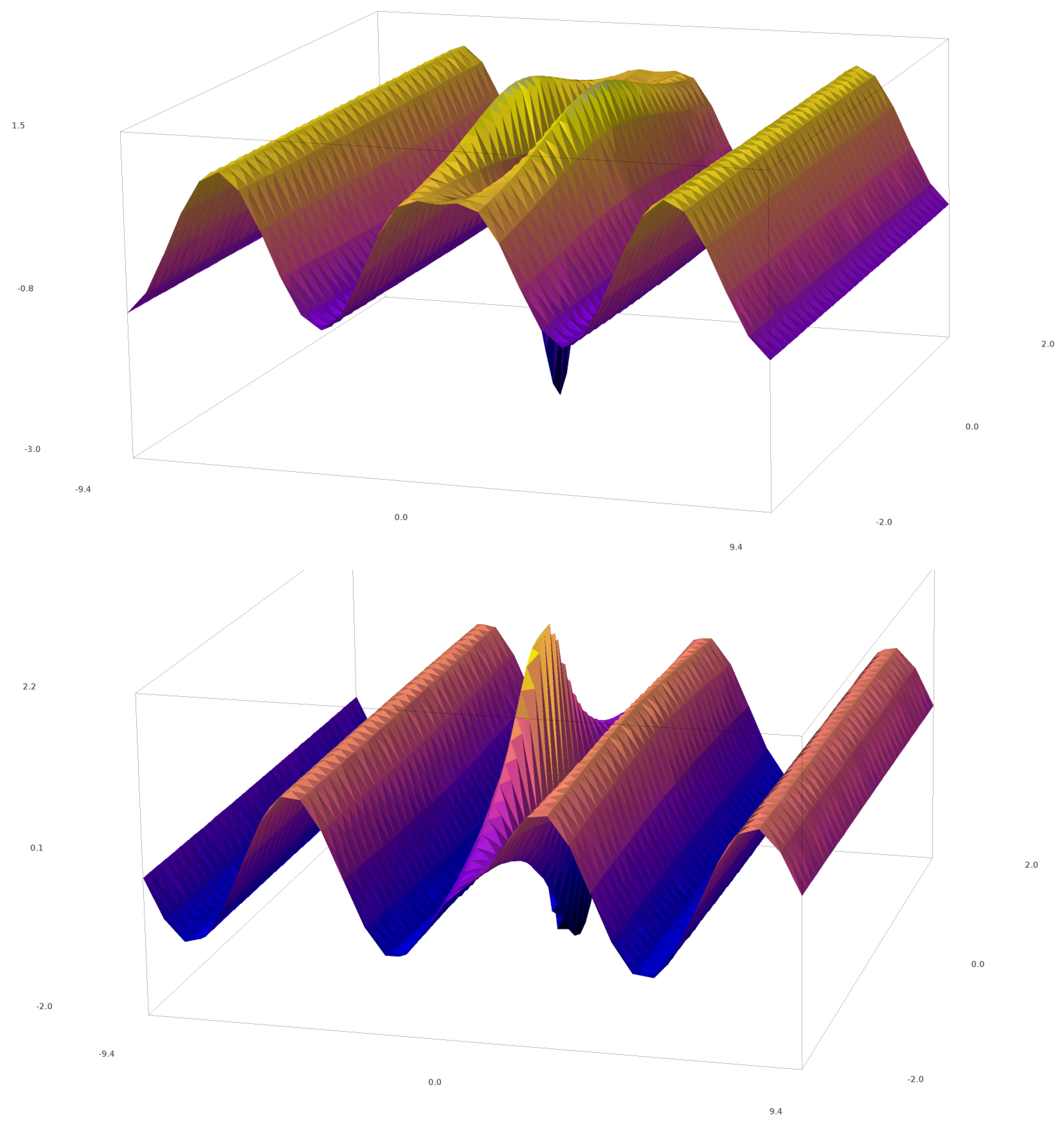
where G, H and Dare the polynomials of the two variables x and t (mentioned above). The first order-solution [19] has the following polynomials: G = 1, H = 2 and , which give the following envelope function (shown in Figure 2):
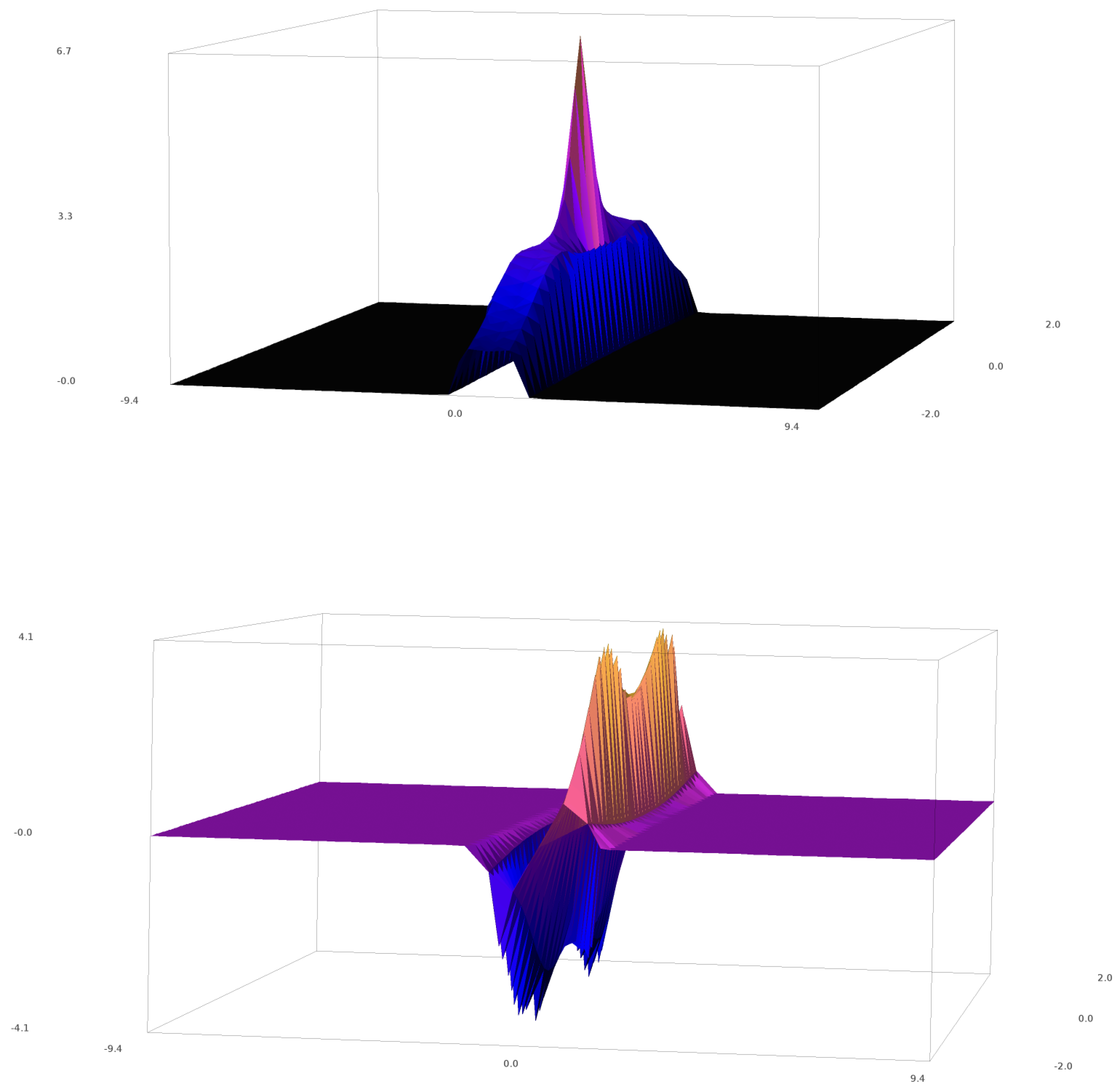
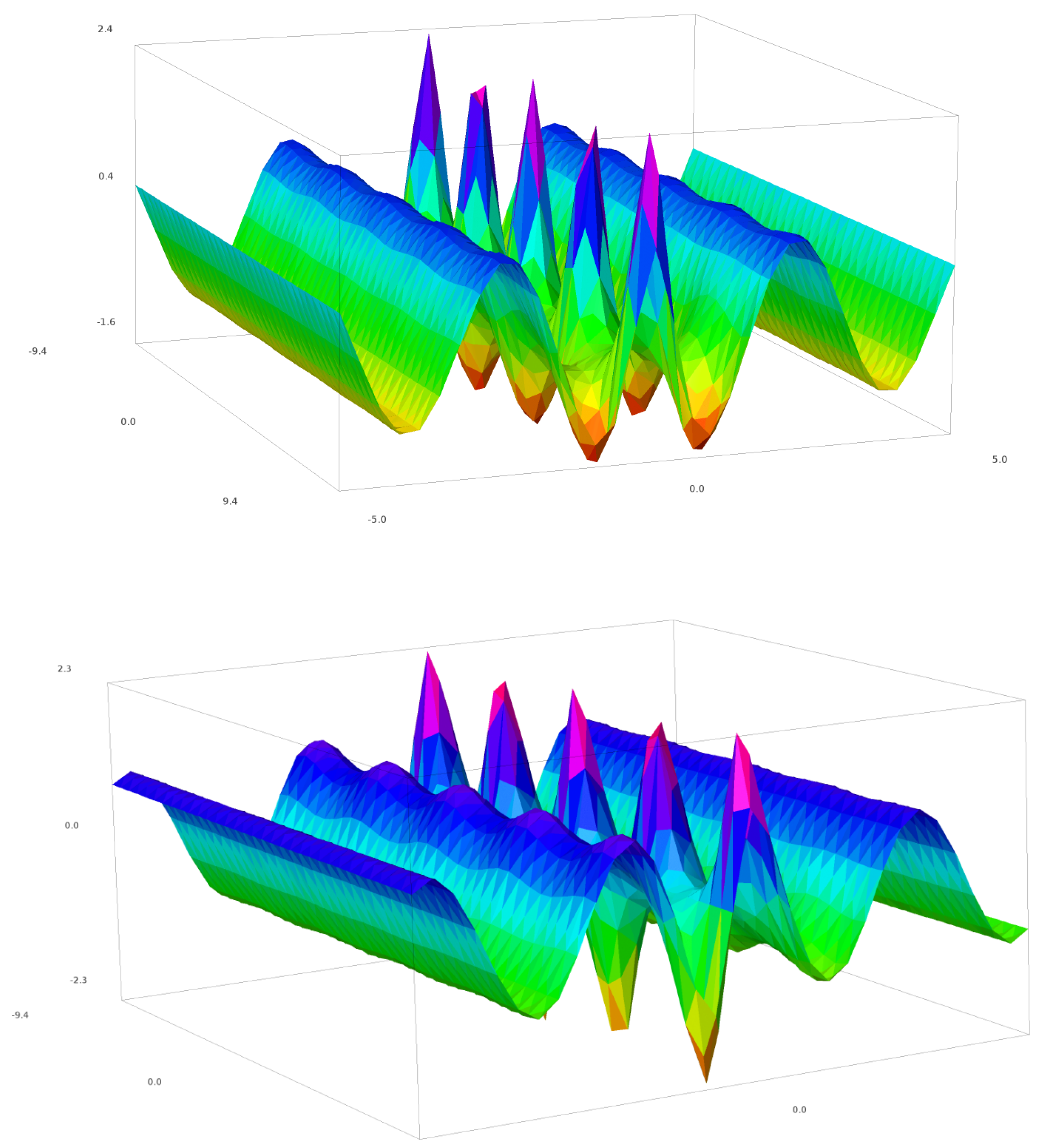
For the second-order solution, [19] identify the vectors r2 and s2 by solving Equations (6) and (7) by using the form of given in (10). This gives the second-order solution:
which is shown in Figure 3. The third and fourth order rational solutions are furthermore calculated and given in [19].
The same hierarchy-dependency is given in the approach by [17], for the transformed vci-NLSE, who define the general solutions for the NLSE in the hierarchical -th order given by:
where each factor is given for the first and second order rational solutions [17]. Similarly to the hierarchy solutions of Akhmediev [19], the increasing order gives higher and higher rogue waves, compared to their surrounding waves. The first and second order rational solutions given in [17] reflect respectively a 3× and 5× rogue wave height, compared to the surrounding waves. For plots of these, refer to [17].
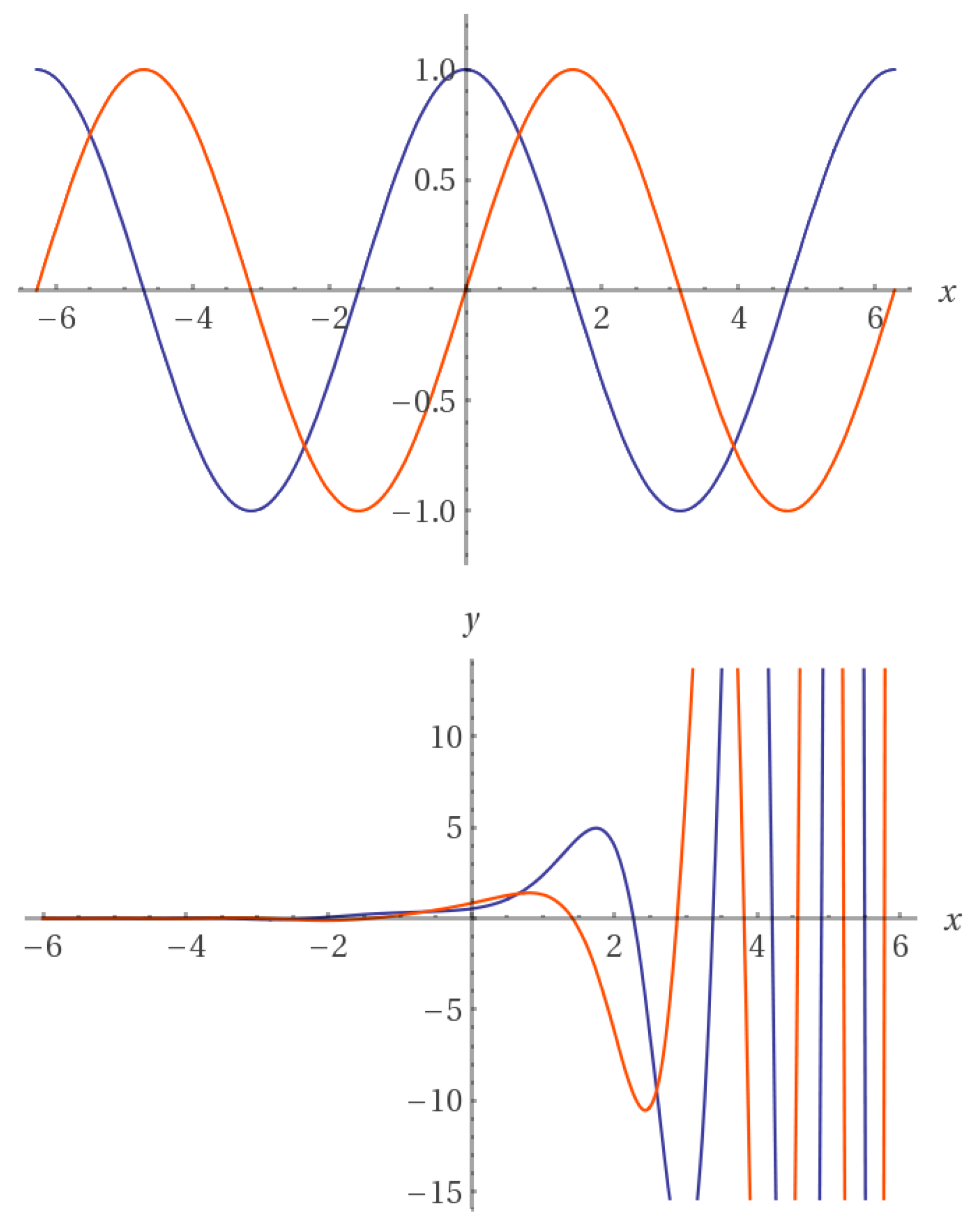
The similarity between (13) and (10) is striking, and both retain the basic form of a complex polynomial multiplied by a complex exponential root function giving soliton solutions. The root functions of (10) and (13) are shown in their generic form in Figure 4, which depicts the distinction between the seed pulse for the regular NLSE and the vci-NLSE, as studied respectively by [17,19] for the rogue wave problem.
The root function for the vci-NLSE (Figure 4) shows its specific pattern of wave accumulation, which is similar to the formation of wave packets. This pattern is conserved with the physical behavior of rogue wave formation, where the rogue wave forms during a focusing phase [51]. Other approaches used to solve the NLSE have been given by [37], who used the inverse scattering method of transformation, which is a generalization of the Fourier analysis. Their solutions differ from the methods discussed above and are periodic and ascribed by a complex envelope function for the deep water train with added higher order terms from the perturbation procedure [37]. One of the solutions is shown in Figure 5, which shows the following variant of the Osborne models:
which is a periodic function in space, derived from the general form given in [37], shown in Figure 5.
3. The Korteweg–de Vries Equation
Wave systems defined by higher order nonlinear PDEs, such as (2), can be solved also by the bilinearization technique [52]. This technique involves the step of transforming the differential equation into a more tractable form by replacing the unknown time- and position-dependent envelope function with a new form [52]. After this replacement has been performed, the bilinearization technique applies Hirota bilinear operators for a modified Bäcklund transformation technique [53], which assists in rewriting the original PDE into a simplified PDE composed of bilinear operators, from which exact soliton solutions can be identified. The most suitable example [52] for the application of the bilinearization technique is on the Korteweg–de Vries (KdV) equation:
where the boundary conditions are that as . The real wavefunction is differentiated according to the spatial and temporal dimensions as denoted. In the bilinearization technique, a transformation of the wavefunction to another form is the first step, where an ideal steady-state form is proposed [52] to:
where:
and and p are arbitrary constants. By the bilinearization technique [52], one can rewrite (16) in the form:
which is converted to its functional form:
with f(x) = 1 + .
The bilinearization technique [52] substitutes (19) into the original KdV Equation (15) and integrates it with respect to x:
which is the original version of the bilinearized variant of the Korteweg–de Vries Equation (15) as derived by [53]. The solution to (20), f(x) = 1+, is defined as a more fundamental quantity than in Equation (18) for the structure of the original nonlinear PDE in Equation (15). In the method of bilinearization, the Hirota bilinear operators are introduced. These are defined by the following definition [53]:
with and being arbitrary positive integers. At this stage, the converted form of the KdV Equation (20) is rewritten as a PDE composed of Hirota operators:
which is a simplified form for the identification of exact solutions using the Bäcklund transformation for the original nonlinear PDE (15). The exact solution structure for the type of Hirota-operator based PDE form (22) of the KdV Equation (15) is given by:
which represents the two-soliton solution to the original KdV Equation (15). and are the functions with the independent variables x and t as given in (16) for each of the solitons, and and , following the same definition for (16) for each soliton. represent the perturbations [52]. The KdV Equation (15) has also been solved by Matveev by identifying positon solutions [54], which exert the same behavior as solitons, such as conserved shape after collision and elastic collision behavior. The positon differs from the soliton in that it has an infinite energy and is therefore not a strong model for oceanic or optical rogue waves. Positons have however a tendency to represent smoother solutions than solitons to the KdV equation and can have very high peaks compared to the wave normal. The KdW equation has also been solved by a nonlinear Fourier method [55,56], which is represented by a superposition of nonlinear oscillatory modes of the wave spectrum. This model, developed by Osborne [55,56], has the capacity to include a large number of non-linear oscillatory patterns, also known as multi-quasi-cnoidal waves, which are used to form the rogue wave by superposition in constructive phases. These solutions to the original KdV Equation (15) include several solitons, depending on the number of degrees of freedom selected for the numerical simulation of the KdV equation. This yields a 3D wave complex composed of solitons and radiation components in the simulated wave train [55].
4. The Extended Dysthe Equation
In 1979, Dysthe [57] developed a modification of the perturbation-based NLSE by adding an additional term to the third-order perturbation variant originally developed by Higgins [58]. Dysthe’s method gave an NLSE variant, known as the extended Dysthe equation, which was shown to have a better agreement with the mean flow response to non-uniformities in deep-water waves. The extended Dysthe equation is given by:
where the inhomogenous component is the fourth-order perturbation defined by Dysthe [57]. Dysthe transformed this equation to standard NLSE using dimensionless variables and added the following perturbation to the general solution:
where and are small real perturbations of the amplitude and phase, respectively. After insertion of (25) in the dimensionless form of (24) and linearizing, Dysthe obtained a simplified system of two PDEs, where the respective plane-wave solutions are in the form:
and:
where K = and , and are selected parameters that satisfy a set of dispersion relations given by Dysthe [57].
The stability of the solutions derived by Dysthe shows that the Dysthe equation represents a more realistic model than the NLSE, given that it does not predict a maximum growth rate for all wavevectors, but only for some wavevectors. This displays that the fourth order perturbation term added to the NLSE gives a considerable improvement to the results relating to the stability of the finite amplitude wave. It is particularly the first derivative by the transformed variables in the x and z dimensions in Equation (24) that contributes to the excellent results of Dysthe. Dysthe and Trulsen [59,60] further developed this equation by including up to the fifth-order of the derivative of the wave amplitude describing the linear dispersive terms and simulated successfully [61] the New Year’s wave [4] using the extended Dysthe equation [57,61].
5. The MMT Model
The MMT equation is a one-dimensional nonlinear dispersion equation, which was originally proposed by Majda, McLaughlin and Tabak [62]. The MMT equation gives soliton-like solutions, which have been analyzed in detail by Zhakarov [63,64,65], and gives four-wave resonant interaction between waves, which, when coupled with large-scale forces and small-scale damping, yields a family of solutions that exhibit direct and inverse cascades [22]. The MMT equation is given by:
where is a complex scalar and is the pseudodifferential operator defined on the real axis through the Fourier transform:
The last term in (28) is the dissipation term, which is tuned to fit ocean waves through the Laplacian operator, D, defined in the Fourier space:
This dissipation term, used by [22], is similar to other dissipation models used by Komen and colleagues [66], who have developed concrete models for simulating large wave groups with focusing and defocusing effects. is the nonlinearity coefficient and corresponds to the focusing phase when <0 and to the defocusing phase when >0. The MMT Equation (28) differs from the standard NLSE in that its family of solutions develops in a more exponential pattern, rather then the Gaussian bell-shaped pattern observed for the solutions for the NLSE [22]. The interesting aspect of this pattern of the spectrum of solutions of the MMT equation is in the mode of formation of the rogue wave, where their energy is transferred from and to the surrounding waves. The solutions are in other words induced by the intermittent formation from the localized rogue event arising out of the regular Gaussian background and collapsing into the surrounding waves. The energy of the rogue wave is transferred to the surroundings and experiences a complete zero-point state, merging completely in the background [22].
The MMT model shows also the formation of quasisolitons, which appear in triple-wave packets, as modeled by Zakharov and Pushkarev [63] and differ from regular solitons in that they radiate the energy backwards towards the preceding amplitudes. This behavior of the solutions may be particularly compatible with the simulation of rogue wave events occurring in regions with strong counter-wind currents, such as in the Agulhas Current [67] or in the regions of the Irish sea [2], which are heavily populated by rogue events, on the passage of the warm waters of the Gulf stream when encountering the frequent low-pressure systems over the Irish sea with counter-wave winds. The quasibreathers or quasisolitons [63] have a root function similar to the Dysthe-type solutions given in (25). Zakharov and Pushkarev [63] approach the solutions in the form:
where and V are constants ( and ) and k is the wavenumber, which is an approximate solution to the soliton-like solution for the MMT model. In this approximation, [63] give k the following form:
which represents a form that gives quasi-soliton solutions [68] to the MMT equation. This form of the solutions to the MMT equation radiates energy backwards to the proceeding amplitudes and represents therefore an energy focusing, which is rather dissimilar from the focusing effects modeled by others for rogue patterns (vide supra). It is interesting to note that backward radiation plays also a central role in the dynamics of the quasi-solitons, and not only for their energy accumulation profile. Using the MMT model, Zakharov and Pushkarev [63] developed also a model for collapses of the rogue event, by using self-similar solutions, and modeled the formation of the wave wedge in the appearing and vanishing state, given by a Fourier space distribution of the wave function. Zakharov and Pushkarev [63] have also used the MMT model to develop a turbulence-based solution for the localized rogue event, using the initial condition in the form of an NLSE soliton:
which shows a conserved action and momentum and an “inner turbulence” localized both in the real and Fourier spaces of the solutions to the modeled envelope function. This “intrinsic turbulence” is described by the authors as affecting the form of its wave spectra, which is irregular and has a stochastic behavior [63]. This model of the rogue wave shows quasi-periodic oscillations with slowly diminishing amplitudes over time, caused by the destruction of rogue wave by the surrounding interference, which the authors denoted as a “quasi-breather”.
6. The Hirota Equation
Multisolitons and breathers for rogue waves have been also successfully modeled [69] by applying the Darboux transformation on the Hirota equation [53]. In their approach, Tao and He [69] developed the Lax pair on the Hirota equation, by using the AKNS [70] procedure to get the Lax pair with the spectral parameters of the Hirota equation given below:
where the Lax pair is expressed as:
giving rise to the extended matrix representation of the operators in the Hirota equation as described by Tao and He [69]. Tao and He further applied the Darboux transformation [43] on the Lax-represented system by using the simple gauge transformation for spectral problems,
where T is the polynomial applied on the parameter given in the Lax pair and is the seed function. Tao and He [69] argue however that regular seed solution as described in the previous sections is too special and makes the rogue wave model not universal enough. Tao and He develop therefore a different seed function compared to Akhmediev and colleagues [19,44], for instance, and develop a more extended form of the seed function by starting from a zero seed solution and a periodic seed solution to construct the complete solutions for the breathers and solitons. At zero seed and with the parameter from the Lax pair, they set the following Hermitian seed pair:
and:
back in the Darboux transformation to get the one-soliton solution:
Tao and He [69] further report the model for the two-soliton solution and finally give the form of the one-soliton breather solution:
where , , are given in [69]. Tao and He finally construct the Rogue wave solutions to the original Hirota equation in (34) by Taylor expansion on the breather solutions in (40). The Taylor expansion is carried out on the variable of the breather solution (40), which is given in [69], and forms the general form of the first order rogue wave of the Hirota equation:
where the polynomials , , are given by Tao and He [69]. The rogue wave model resulting from this form is more general than the model given by Akhmediev and colleagues [71] on the Hirota equation. This difference is caused by the appearance of several parameters related to the eigenvalues of the Lax pairs and gives however a possibility to tune more finely the model to experiments on rogue waves. This advantage of the model by Tao and He increases the ability to modulate the precision of reproducing a rogue wave model by calculations. Tao and He’s method grants also the possibility of calculating higher order rogue wave solutions to the Hirota equation by determinant representation of the Darboux transform, which was carried out in a subsequent work [72].
7. The Ablowitz–Musslimani Models: Non-Local Rogue Waves
Another critical method for modeling rogue waves was developed by Ablowitz and Musslimani [73,74,75,76] and uses nonlocal integrable models of the NLSE (1) and KdV (15) equations, where the resulting wave is derived by reverse space-time symmetry. The model evolves by establishing integrability by an infinite number of constants of motion or an infinite number of conservation laws. By this, the method uses a compatible pair of linear equations (similar to the Lax pair in the Hirota equation in (35)) with the nonlinear integrable equation. The method by Ablowitz and Musslimani differs from the Hirota method in that the pair of linear equations represent the scattering problem and the evolution of the scattering data [73,76]. Furthermore, the method by Ablowitz and Musslimani is different from others in that it constructs an inverse scattering problem also known as a linear Riemann–Hilbert problem, which gives the solution to the nonlinear PDE with dependency on time.
The approach by Ablowitz and Musslimani [73] starts by linearizing the equation:
where one can immediately observe the existence of a Hermitian pair with reverse directional variables. This form, where reverse variables are used, defines the nonlocal property of the equation and has the advantage that the equation remains invariant in time and space, after the complex conjugate is taken. Hence, the nonlocal equation is parity- and time-symmetric (-symmetric), which prevents the equation from yielding different results by a self-induced potential.
An exemplary Lax pair is given in [77] as:
where is the two-component vector and is a special parameter, while A and B are complex functions. Ablowitz and Musslimani use this step specific compatibility conditions [78] to transform the original PDE in (42) (i.e., ) and gain the simplified PDE pair:
which yields the original form in Equation (42). Ablowitz and Musslimani further define the nonlocality by using a specific symmetry reduction:
This step is particularly characteristic of Ablowitz–Musslimani models [73,74,75,76], from which the new class of nonlocal integrable evolution equations with the nonlocal NLSE hierarchy is directly derived.
The aforementioned property of conserved quantities and conservation laws is also characteristic of Ablowitz–Musslimani models [73,75]. Here, they define a set of eigenfunctions that obey specific boundary conditions [73]. The eigenfunctions are very similar to the seed functions used by other groups and, when inserted in the Lax pair, yield a Riccati model of the conservation quantities. This yields the global conservation laws, which are given in [73] by:
which are real integrable Hamiltonians. Ablowitz and Musslimani [73] derive furthermore local conservation laws defined by the equations:
which are used to develop the framework for the direct scattering problem and the inverse scattering problem, where the scattering data are given by specific scattering matrices. The same symmetry is also in the problem of the potential and in the eigenfunction and leads naturally to the same symmetry relation in the scattering matrices, which is given by:
and:
where is a 2 × 2 matrix with zeros in the diagonal and one, on the lower and upper diagonal, respectively. For the inverse scattering problem, Ablowitz and Musslimani [73] account for the symmetry condition by considering the set of basis terms as a left scattering problem and supplement these terms with the equivalent right-scattering problem, from which they formulate the Riemann–Hilbert problem and find the linear integral equations that govern the functions M and in (50). These equations are given by:
where and are the reflection coefficients. The terms and are the conservation law Hamiltonians applied symmetrically. From this stage, Ablowitz and Musslimani [73] derive a linear algebraic integral system of equations that solves the inverse problem for the eigenfunctions and .
The resulting soliton solutions of the Ablowitz–Musslimani model hence assume the form:
which represents a family of solutions defined by the four independent parameters, which have a dynamic relationship with the time variable and which gradually develop a singularity in a finite time period, at x = 0, where is given by:
Equation (55) is a critical form of the time-variable, which distinguishes the method of Ablowitz–Musslimani [73,74,75,76,77,78] from other rogue wave models and adds a non-linear evolution of the rogue wave. Ablowitz and Musslimani have also most recently developed a new model that includes nonlocal rogue waves with nonzero background, which provide a more realistic view of the rogue wave, which focuses energy from neighboring waves [79].
Solutions to the Ablowitz–Musslimani model (42) were also developed by Yang and Yang [80], who used the Darboux transformation method on the PDE coupled with the Bäcklund transformation on the potential functions, identifying three types of rogue waves from the Ablowitz–Musslimani picture. Yang and Yang expanded the solutions to polynomials using Schur polynomials [80]. This analysis of the Ablowitz–Musslimani model showed greater variation in the rogue waves compared to the regular NLSE, where the variations were represented by the terms in the denominator of the soliton solutions.
The parity-time symmetry potential of the Ablowitz–Musslimani equations has also been studied by Yu [81] very recently, who obtained discrete rogue wave solutions with three free parameters (refer to Equation (54) for similarities). Yu studied in particular the effect that the dispersion of the parity-time symmetry has on the solutions, as well as the effect of the coefficients and the parameters. Yu [81] used the Darboux transformation method in a similar fashion to Yang and Yang [80] to derive different forms of solitons with different heights, which were defined by two of the three free parameters in the solution ( and in Equation (54)). Yu [81] also assessed the stability of rogue waves over a specific period of time and included a modulation instability coefficient that allows the modeling of several discrete solutions that represent various stages of rogue wave formation (appearing suddenly and disappearing suddenly), a property of rogue waves also reported by Akhmediev and colleagues [18,19,20]. Finally, Yu modeled rogue waves that appear rapidly and do not disappear. This latter model may be particularly relevant to describe rogue events during low-pressure systems at open sea, which have been reported in several cases to give stable rogue waves with a long lifetime (i.e., the rogue waves reported in the study by Munk [35]).
8. Conclusions
A survey of various mathematical models for representing rogue waves has herein been carried out to the maximum extent of including the most applied, as well as most recent models. The overall survey yields a perspective that delineates the common traits between the methods. This survey also shows how novel and emerging models allow for better modeling of rogue waves, by including several parameters associated with the evolution of the rogue waves, such as the duration, the height and other particular properties that a rogue event can display when occurring in oceans, optical systems or even in the atmosphere. The results show also that the new versatile forms of the older models (MMT and Dysthe) can be furthermore adapted and studied numerically in upcoming papers, particularly with relevance to counter-wave winds, which frequently occur on the Gulf Current off the Irish coast and on the western Norwegian coast during northeast and north winds, respectively. By the overall review of the various methods, a theorem is suggested for describing the origin of rogue waves in the ocean. The theorem suggests that a rogue wave in the ocean can be formed whenever there is a momentaneous surplus of energy perturbed on the momentum or in the kinetic term of a wave train, induced either by a sudden change in the atmosphere leading to strong winds appearing suddenly over large volumes of water, or induced by a collision of large volumes of water with highly different temperatures and densities, or finally, as often observed, a rogue event occurs by the constructive overlap of waves, in opposite directions, in traverse directions or running in the same direction, and its duration is determined, when occurring in the same direction, by the slight deviations in the momenta of the overlapping waves. Future work will be the submission of a project proposal for predicting rogue waves for off-shore structures, currently under development for the Norwegian Research Council.
Funding
This research received no funding.
Conflicts of Interest
The author declares no conflict of interest.
Abbreviations
The following abbreviations are used in this manuscript:
| MMT | Majda–McLaughlin–Tabak |
| AKNS | Ablowitz–Kaup–Newell–Segur |
References
- Lehner, S.; Schulz-Stellenfleth, J.; Niedermeier, A.; Horstmann, J.; Rosenthal, W. Extreme waves detected by satellite borne synthetic aperture radar. In Proceedings of the ASME 2002 21st International Conference on Offshore Mechanics and Arctic Engineering, Oslo, Norway, 23–28 June 2002; American Society of Mechanical Engineers: New York, NY, USA, 2002; pp. 251–256. [Google Scholar]
- Rosenthal, W.; Lehner, S. Rogue waves: Results of the MaxWave project. J. Offshore Mech. Arct. Eng. 2008, 130, 021006. [Google Scholar] [CrossRef]
- Didenkulova, I.; Slunyaev, A.; Pelinovsky, E.; Kharif, C. Freak waves in 2005. Nat. Hazards Earth Syst. Sci. 2006, 6, 1007–1015. [Google Scholar] [CrossRef] [Green Version]
- Haver, S. A possible freak wave event measured at the Draupner Jacket January 1 1995. In Proceedings of the 2004 Rogue Waves, Brest, France, 20–22 October 2004; pp. 1–8. [Google Scholar]
- Stansell, P. Distributions of freak wave heights measured in the North Sea. Appl. Ocean Res. 2004, 26, 35–48. [Google Scholar] [CrossRef]
- Dysthe, K.; Krogstad, H.E.; Müller, P. Oceanic rogue waves. Annu. Rev. Fluid Mech. 2008, 40, 287–310. [Google Scholar] [CrossRef]
- Weisse, R. Marine Climate and Climate Change: Storms, Wind Waves and Storm Surges; Springer Science & Business Media: Berlin, Germany, 2010. [Google Scholar]
- Solli, D.; Ropers, C.; Koonath, P.; Jalali, B. Optical rogue waves. Nature 2007, 450, 1054. [Google Scholar] [CrossRef] [PubMed]
- Stenflo, L.; Marklund, M. Rogue waves in the atmosphere. J. Plasma Phys. 2010, 76, 293–295. [Google Scholar] [CrossRef]
- Moslem, W.; Shukla, P.; Eliasson, B. Surface plasma rogue waves. Europhys. Lett. 2011, 96, 25002. [Google Scholar] [CrossRef]
- Tlidi, M.; Gandica, Y.; Sonnino, G.; Averlant, E.; Panajotov, K. Self-Replicating spots in the brusselator model and extreme events in the one-dimensional case with delay. Entropy 2016, 18, 64. [Google Scholar] [CrossRef]
- Kibler, B.; Fatome, J.; Finot, C.; Millot, G.; Dias, F.; Genty, G.; Akhmediev, N.; Dudley, J.M. The Peregrine soliton in nonlinear fibre optics. Nat. Phys. 2010, 6, 790–795. [Google Scholar] [CrossRef] [Green Version]
- Levi-Civita, T. Determination rigoureuse des ondes permanentes d’ampleur finie. Math. Ann. 1925, 93, 264–314. [Google Scholar] [CrossRef]
- Nekrasov, A. On waves of permanent type. Izv. Ivanovo-Voznesensk. Politekhn. Inst. 1921, 3, 52–65. [Google Scholar]
- Smith, R. Giant waves. J. Fluid Mech. 1976, 77, 417–431. [Google Scholar] [CrossRef]
- Zakharov, V.E. Collapse of Langmuir waves. Sov. Phys. JETP 1972, 35, 908–914. [Google Scholar]
- Dai, C.Q.; Wang, Y.Y.; Tian, Q.; Zhang, J.F. The management and containment of self-similar rogue waves in the inhomogeneous nonlinear Schrödinger equation. Ann. Phys. 2012, 327, 512–521. [Google Scholar] [CrossRef]
- Akhmediev, N.; Soto-Crespo, J.M.; Ankiewicz, A. Extreme waves that appear from nowhere: on the nature of rogue waves. Phys. Lett. A 2009, 373, 2137–2145. [Google Scholar] [CrossRef]
- Akhmediev, N.; Ankiewicz, A.; Soto-Crespo, J. Rogue waves and rational solutions of the nonlinear Schrödinger equation. Phys. Rev. E 2009, 80, 026601. [Google Scholar] [CrossRef] [PubMed]
- Akhmediev, N.; Ankiewicz, A.; Soto-Crespo, J.; Dudley, J.M. Rogue wave early warning through spectral measurements? Phys. Lett. A 2011, 375, 541–544. [Google Scholar] [CrossRef] [Green Version]
- Chabchoub, A.; Hoffmann, N.; Branger, H.; Kharif, C.; Akhmediev, N. Experiments on wind-perturbed rogue wave hydrodynamics using the Peregrine breather model. Phys. Fluids 2013, 25, 101704. [Google Scholar] [CrossRef] [Green Version]
- Cousins, W.; Sapsis, T.P. Quantification and prediction of extreme events in a one-dimensional nonlinear dispersive wave model. Phys. D Nonlinear Phenom. 2014, 280, 48–58. [Google Scholar] [CrossRef] [Green Version]
- Cousins, W.; Sapsis, T.P. Unsteady evolution of localized unidirectional deep-water wave groups. Phys. Rev. E 2015, 91, 063204. [Google Scholar] [CrossRef] [PubMed]
- Cousins, W.; Sapsis, T.P. Reduced-order precursors of rare events in unidirectional nonlinear water waves. J. Fluid Mech. 2016, 790, 368–388. [Google Scholar] [CrossRef] [Green Version]
- Tlidi, M.; Panajotov, K. Two-dimensional dissipative rogue waves due to time-delayed feedback in cavity nonlinear optics. Chaos Interdiscip. J. Nonlinear Sci. 2017, 27, 013119. [Google Scholar] [CrossRef] [PubMed] [Green Version]
- Lugiato, L.A.; Lefever, R. Spatial dissipative structures in passive optical systems. Phys. Rev. Lett. 1987, 58, 2209. [Google Scholar] [CrossRef] [PubMed]
- Panajotov, K.; Clerc, M.G.; Tlidi, M. Spatiotemporal chaos and two-dimensional dissipative rogue waves in Lugiato-Lefever model. Eur. Phys. J. D 2017, 71, 176. [Google Scholar] [CrossRef]
- Akhmediev, N.; Kibler, B.; Baronio, F.; Belić, M.; Zhong, W.P.; Zhang, Y.; Chang, W.; Soto-Crespo, J.M.; Vouzas, P.; Grelu, P.; et al. Roadmap on optical rogue waves and extreme events. J. Opt. 2016, 18, 063001. [Google Scholar] [CrossRef] [Green Version]
- Dai, C.; Wang, Y.; Yan, C. Chirped and chirp-free self-similar cnoidal and solitary wave solutions of the cubic-quintic nonlinear Schrödinger equation with distributed coefficients. Opt. Commun. 2010, 283, 1489–1494. [Google Scholar] [CrossRef]
- Haghgoo, S.; Ponomarenko, S.A. Self-similar pulses in coherent linear amplifiers. Optics Express 2011, 19, 9750–9758. [Google Scholar] [CrossRef] [PubMed]
- Kruglov, V.; Peacock, A.; Harvey, J. Exact self-similar solutions of the generalized nonlinear Schrödinger equation with distributed coefficients. Phys. Rev. Lett. 2003, 90, 113902. [Google Scholar] [CrossRef] [PubMed]
- Kruglov, V.; Peacock, A.; Harvey, J. Exact solutions of the generalized nonlinear Schrödinger equation with distributed coefficients. Phys. Rev. E 2005, 71, 056619. [Google Scholar] [CrossRef] [PubMed]
- Fermann, M.; Kruglov, V.; Thomsen, B.; Dudley, J.; Harvey, J. Self-similar propagation and amplification of parabolic pulses in optical fibers. Phys. Rev. Lett. 2000, 84, 6010. [Google Scholar] [CrossRef] [PubMed]
- Hamedi, H.R. Optical bistability and multistability via magnetic field intensities in a solid. Appl. Opt. 2014, 53, 5391–5397. [Google Scholar] [CrossRef] [PubMed]
- Munk, W.; Snodgrass, F. Measurements of southern swell at Guadalupe Island. Deep Sea Res. 1957, 4, 272–286. [Google Scholar] [CrossRef]
- Kruglov, V.; Peacock, A.; Dudley, J.; Harvey, J. Self-similar propagation of high-power parabolic pulses in optical fiber amplifiers. Opt. Lett. 2000, 25, 1753–1755. [Google Scholar] [CrossRef] [PubMed]
- Osborne, A.R.; Onorato, M.; Serio, M. The nonlinear dynamics of rogue waves and holes in deep-water gravity wave trains. Phys. Lett. A 2000, 275, 386–393. [Google Scholar] [CrossRef]
- Zakharov, V.E. Stability of periodic waves of finite amplitude on the surface of a deep fluid. J. Appl. Mech. Tech. Phys. 1968, 9, 190–194. [Google Scholar] [CrossRef]
- Serkin, V.; Hasegawa, A.; Belyaeva, T. Nonautonomous solitons in external potentials. Phys. Rev. Lett. 2007, 98, 074102. [Google Scholar] [CrossRef] [PubMed]
- Dai, C.Q.; Wang, D.S.; Wang, L.L.; Zhang, J.F.; Liu, W. Quasi-two-dimensional Bose–Einstein condensates with spatially modulated cubic–quintic nonlinearities. Ann. Phys. 2011, 326, 2356–2368. [Google Scholar] [CrossRef]
- Peregrine, D. Water waves, nonlinear Schrödinger equations and their solutions. ANZIAM J. 1983, 25, 16–43. [Google Scholar] [CrossRef]
- Zakharov, V.; Shabat, A. Interaction between solitons in a stable medium. Sov. Phys. JETP 1973, 37, 823–828. [Google Scholar]
- Matveev, V.B.; Matveev, V. Darb. Trans. Solitons; Springer-Verlag: Berlin, Germany, 1991. [Google Scholar]
- Akhmediev, N.; Korneev, V. Modulation instability and periodic solutions of the nonlinear Schrödinger equation. Theor. Math. Phys. 1986, 69, 1089–1093. [Google Scholar] [CrossRef]
- Dysthe, K.B.; Trulsen, K. Note on breather type solutions of the NLS as models for freak-waves. Phys. Scr. 1999, 1999, 48. [Google Scholar] [CrossRef]
- Voronovich, V.V.; Shrira, V.I.; Thomas, G. Can bottom friction suppress ‘freak wave’formation? J. Fluid Mech. 2008, 604, 263–296. [Google Scholar] [CrossRef]
- Benjamin, T.B.; Feir, J. The disintegration of wave trains on deep water Part 1. Theory. J. Fluid Mech. 1967, 27, 417–430. [Google Scholar] [CrossRef]
- Bespalov, V.; Talanov, V. Filamentary structure of light beams in nonlinear liquids. ZhETF Pisma Redaktsiiu 1966, 3, 471. [Google Scholar]
- Kim, D.S.; Markowsky, G.; Lee, S.G. Mobile Sage-Math for linear algebra and its application. Electron. J. Math. Technol. 2010, 4, 285–298. [Google Scholar]
- SageMath Mathematics Software, Version 6.5. 2015. Available online: http://www.sagemath.org/ (accessed on 5 June 2017).
- Kharif, C.; Pelinovsky, E. Physical mechanisms of the rogue wave phenomenon. Eur. J. Mech. B Fluids 2003, 22, 603–634. [Google Scholar] [CrossRef] [Green Version]
- Matsuno, Y. Bilinear Transformation Method; Elsevier: New York, NY, USA, 1984. [Google Scholar]
- Hirota, R. A new form of Bäcklund transformations and its relation to the inverse scattering problem. Prog. Theor. Phys. 1974, 52, 1498–1512. [Google Scholar] [CrossRef]
- Matveev, V.B. Positons: Slowly decreasing analogues of solitons. Theor. Math. Phys. 2002, 131, 483–497. [Google Scholar] [CrossRef]
- Osborne, A. Soliton physics and the periodic inverse scattering transform. Phys. D Nonlinear Phenom. 1995, 86, 81–89. [Google Scholar] [CrossRef]
- Osborne, A. Solitons in the periodic Korteweg–de Vries equation, the FTHETA-function representation, and the analysis of nonlinear, stochastic wave trains. Phys. Rev. E 1995, 52, 1105. [Google Scholar] [CrossRef]
- Dysthe, K.B. Note on a modification to the nonlinear Schrödinger equation for application to deep water waves. Proc. R. Soc. Lond. A 1979, 369, 105–114. [Google Scholar] [CrossRef]
- Longuet-Higgins, M. The instability of gravity waves of infinite amplitude in deep water. II. Subharmonics. Proc. R. Soc. Lond. A 1978, 360, 489–506. [Google Scholar] [CrossRef]
- Trulsen, K.; Dysthe, K. Freak waves—A three-dimensional wave simulation. In Proceedings of the 21st Symposium on Naval Hydrodynamics, Trondheim, Norway, 24–28 June 1996; National Academy Press: Washington, DC, USA, 1997; Volume 550, p. 558. [Google Scholar]
- Trulsen, K.; Dysthe, K.B. A modified nonlinear Schrödinger equation for broader bandwidth gravity waves on deep water. Wave Motion 1996, 24, 281–289. [Google Scholar] [CrossRef]
- Trulsen, K.; Kliakhandler, I.; Dysthe, K.B.; Velarde, M.G. On weakly nonlinear modulation of waves on deep water. Phys. Fluids 2000, 12, 2432–2437. [Google Scholar] [CrossRef]
- Majda, A.; McLaughlin, D.; Tabak, E. A one-dimensional model for dispersive wave turbulence. J. Nonlinear Sci. 1997, 7, 9–44. [Google Scholar] [CrossRef]
- Pushkarev, A.; Zakharov, V. Quasibreathers in the MMT model. Phys. D Nonlinear Phenom. 2013, 248, 55–61. [Google Scholar] [CrossRef] [Green Version]
- Zakharov, V.; Dias, F.; Pushkarev, A. One-dimensional wave turbulence. Phys. Rep. 2004, 398, 1–65. [Google Scholar] [CrossRef]
- Zakharov, V.; Guyenne, P.; Pushkarev, A.; Dias, F. Wave turbulence in one-dimensional models. Phys. D Nonlinear Phenom. 2001, 152, 573–619. [Google Scholar] [CrossRef] [Green Version]
- Komen, G.J.; Cavaleri, L.; Donelan, M. Dynamics and Modelling of Ocean Waves; Cambridge University Press: Cambridge, UK, 1996. [Google Scholar]
- Lavrenov, I. The wave energy concentration at the Agulhas current off South Africa. Nat. hazards 1998, 17, 117–127. [Google Scholar] [CrossRef]
- Zakharov, V.; Kuznetsov, E. Optical solitons and quasisolitons. J. Exp. Theor. Phys. 1998, 86, 1035–1046. [Google Scholar] [CrossRef]
- Tao, Y.; He, J. Multisolitons, breathers, and rogue waves for the Hirota equation generated by the Darboux transformation. Phys. Rev. E 2012, 85, 026601. [Google Scholar] [CrossRef] [PubMed]
- Ablowitz, M.J.; Kaup, D.J.; Newell, A.C.; Segur, H. Method for solving the sine-Gordon equation. Phys. Rev. Lett. 1973, 30, 1262. [Google Scholar] [CrossRef]
- Ankiewicz, A.; Soto-Crespo, J.; Akhmediev, N. Rogue waves and rational solutions of the Hirota equation. Phys. Rev. E 2010, 81, 046602. [Google Scholar] [CrossRef] [PubMed]
- He, J.; Zhang, H.; Wang, L.; Porsezian, K.; Fokas, A. Generating mechanism for higher-order rogue waves. Phys. Rev. E 2013, 87, 052914. [Google Scholar] [CrossRef] [PubMed]
- Ablowitz, M.J.; Musslimani, Z.H. Integrable nonlocal nonlinear Schrödinger equation. Phys. Rev. Lett. 2013, 110, 064105. [Google Scholar] [CrossRef] [PubMed]
- Ablowitz, M.J.; Musslimani, Z.H. Inverse scattering transform for the integrable nonlocal nonlinear Schrödinger equation. Nonlinearity 2016, 29, 915. [Google Scholar] [CrossRef]
- Ablowitz, M.J.; Musslimani, Z.H. Integrable nonlocal nonlinear equations. Stud. Appl. Math. 2017, 139, 7–59. [Google Scholar] [CrossRef]
- Ablowitz, M.J.; Musslimani, Z.H. Integrable discrete P T symmetric model. Phys. Rev. E 2014, 90, 032912. [Google Scholar] [CrossRef] [PubMed]
- Musslimani, Z.; Makris, K.G.; El-Ganainy, R.; Christodoulides, D.N. Optical Solitons in P T Periodic Potentials. Phys. Rev. Lett. 2008, 100, 030402. [Google Scholar] [CrossRef] [PubMed]
- Ablowitz, M.J.; Chakravarty, S.; Takhtajan, L.A. A self-dual Yang-Mills hierarchy and its reductions to integrable systems in 1+1 and 2+1 dimensions. Commun. Math. Phys. 1993, 158, 289–314. [Google Scholar] [CrossRef]
- Ablowitz, M.J.; Luo, X.D.; Musslimani, Z.H. Inverse scattering transform for the nonlocal nonlinear Schrödinger equation with nonzero boundary conditions. J. Math. Phys. 2018, 59, 011501. [Google Scholar] [CrossRef] [Green Version]
- Yang, B.; Yang, J. General rogue waves in the nonlocal PT-symmetric nonlinear Schrodinger equation. arXiv, 2017; arXiv:1711.05930. [Google Scholar]
- Yu, F. Dynamics of nonautonomous discrete rogue wave solutions for an Ablowitz–Musslimani equation with PT-symmetric potential. Chaos Interdiscip. J. Nonlinear Sci. 2017, 27, 023108. [Google Scholar] [CrossRef] [PubMed]
Figure 1.
The laser readings of the most extreme rogue wave registered (top), which hit the the North Alwyn platform east of Shetland [5], reaching 18.04 m and a ratio of 3.19× the surrounding waves. (Bottom) The New Years wave registered in 1995 on the Draupner platform in the North Sea.
Figure 1.
The laser readings of the most extreme rogue wave registered (top), which hit the the North Alwyn platform east of Shetland [5], reaching 18.04 m and a ratio of 3.19× the surrounding waves. (Bottom) The New Years wave registered in 1995 on the Draupner platform in the North Sea.

Figure 2.
The plot of , the first-order solution to the standard NLSE [19]. Real and imaginary parts shown respectively above and below. Plotted with SageMATH [49,50].

Figure 3.
The plot of , the second-order solution to the standard NLSE [19]. Real and imaginary parts shown respectively above and below. Plotted with SageMATH [49,50].

Figure 4.
The root functions for the standard NLSE and the inhomogenous variable coefficient NLSE. (Top) The seed impulse used in the solutions to the standard NLSE, [19]. (Bottom) A generic form of the seed impulse used in the solutions of the inhomogenous variable coefficient NLSE [17] . Real part (blue) and imaginary part (red).


© 2018 by the author. Licensee MDPI, Basel, Switzerland. This article is an open access article distributed under the terms and conditions of the Creative Commons Attribution (CC BY) license (http://creativecommons.org/licenses/by/4.0/).
Share and Cite
MDPI and ACS Style
Manzetti, S. Mathematical Modeling of Rogue Waves: A Survey of Recent and Emerging Mathematical Methods and Solutions. Axioms 2018, 7, 42. https://doi.org/10.3390/axioms7020042
AMA Style
Manzetti S. Mathematical Modeling of Rogue Waves: A Survey of Recent and Emerging Mathematical Methods and Solutions. Axioms. 2018; 7(2):42. https://doi.org/10.3390/axioms7020042
Chicago/Turabian StyleManzetti, Sergio. 2018. "Mathematical Modeling of Rogue Waves: A Survey of Recent and Emerging Mathematical Methods and Solutions" Axioms 7, no. 2: 42. https://doi.org/10.3390/axioms7020042
Note that from the first issue of 2016, this journal uses article numbers instead of page numbers. See further details here.