Multiple Estimation Architecture in Discrete-Time Adaptive Mixing Control †

Informatics & Telematics Institute, Center for Research and Technology Hellas (ITI-CERTH), Thessaloniki, 57001, Greece
†
This work has been supported by the European Commission FP7-ICT-5-3.5, Engineering of Networked Monitoring and Control Systems, under the contract #257806 AGILE.
Machines 2013, 1(1), 33-49; https://doi.org/10.3390/machines1010033
Submission received: 11 March 2013
/
Revised: 29 April 2013
/
Accepted: 20 May 2013
/
Published: 29 May 2013
(This article belongs to the Special Issue Advances in Control Engineering)
Abstract
:Adaptive mixing control (AMC) is a recently developed control scheme for uncertain plants, where the control action coming from a bank of precomputed controller is mixed based on the parameter estimates generated by an on-line parameter estimator. Even if the stability of the control scheme, also in the presence of modeling errors and disturbances, has been shown analytically, its transient performance might be sensitive to the initial conditions of the parameter estimator. In particular, for some initial conditions, transient oscillations may not be acceptable in practical applications. In order to account for such a possible phenomenon and to improve the learning capability of the adaptive scheme, in this paper a new mixing architecture is developed, involving the use of parallel parameter estimators, or multi-estimators, each one working on a small subset of the uncertainty set. A supervisory logic, using performance signals based on the past and present estimation error, selects the parameter estimate to determine the mixing of the controllers. The stability and robustness properties of the resulting approach, referred to as multi-estimator adaptive mixing control (Multi-AMC), are analytically established. Besides, extensive simulations demonstrate that the scheme improves the transient performance of the original AMC with a single estimator. The control scheme and the analysis are carried out in a discrete-time framework, for easier implementation of the method in digital control.
1. Introduction
It is well known that, in feedback control design, unknown values of the physical variables of the plant dynamics may lead to a large parametric uncertainty that cannot be handled by a single fixed LTI controller, e.g., and μ-synthesized controllers. The aim of adaptive control is to introduce adaptation mechanisms in the control action in order to handle parametric uncertainties much larger than those that robust control can handle. In the last decades the interest toward multiple model adaptive control architectures has grown, due to the capability to combine tools from adaptive control and robust non-adaptive control in order to handle plants with large parametric and other uncertainties [1,2,3,4,5,6,7,8]. The multiple model architecture comprises a multicontroller consisting of a family of precomputed candidate controllers and some logic that influences the control by selecting the candidate controllers based on processed plant input/output data. The use of precomputed controllers allows the controller design to be performed using well-established tools from LTI theory. Besides, the problem of stabilizability encountered in adaptive control [9,10], where at some time instants the online calculation of finite controller gains is not possible due to singularities, is completely avoided.
A recent adaptive control scheme involving the use of precalculated candidate controllers is adaptive control with mixing (AMC), developed both for continuous-time [11] and discrete-time SISO plants [12]. By monitoring the plant’s input/output data, the supervisor determines the participation level of each candidate controller based on real-time estimates of the unknown parameter vector, and “mixes" the candidate control actions. In the mixing scheme the learning is entrusted to the adaptive law, whose performance depends on the initial conditions. If the I/O data that the on-line adaptive law processes provide little information about the unknown plant dynamics, or if the true parameter vector is far from the initial estimated parameter vector, some undesirable transient can occur before the regulation/tracking task is achieved. In order to account for such a possible phenomenon, a new AMC architecture is developed, involving the use of parallel parameter estimators, or multi-estimators, each one working on a small subset of the uncertainty set. Every parameter estimator differs from the others for its initial condition , and for the subset in which the parameter estimate is projected. A hysteresis switching logic orchestrates the decision of the best estimate among all parallel parameter estimates at each time t.
The resulting AMC scheme, called Multi-estimator AMC, or Multi-AMC, is here established both theoretically and via simulations, to face regulation and tracking problems, for discrete-time SISO uncertain plants. The control scheme is developed in a discrete-time framework, for an easier implementation of the algorithm in digital control. It is shown that the Multi-AMC enjoys the same stability and robustness properties of AMC with one estimator: in the ideal case, when no disturbances or unmodeled dynamics are present, the tracking error converges to zero. The Multi-AMC is also robust with respect to unmodeled dynamics and bounded disturbances: in such a case, all the closed-loop signals are bounded and the mean-square tracking error is of the order of magnitude of the modeling error and the bounded disturbance. While improvements in transient performance with respect to the single estimator case are difficult if at all possible to establish analytically, extensive simulations are used to demonstrate consistent improvements in performance due to the proposed Multi-AMC scheme.
The paper is organized as follows. The problem formulation is exposed in Section 2. Section 3 deals with the multicontroller and the mixing strategy, and the parallel estimation architecture and switching logic are presented in Section 4. The main theorem dealing with stability and stability robustness of the multiple-estimator adaptive mixing control scheme is presented in Section 5. In Section 6 a numerical example is used to show the effectiveness of the method, together with its faster learning and better transients behavior compared with the use of a single on-line estimator.
2. Problem Formulation: Uncertain Plant
Consider the uncertain discrete-time LTI SISO plant
where represents the nominal plant; the vector contains the unknown parameters of ; ; ; is an unknown multiplicative perturbation; and d is a bounded input disturbance, i.e., , .
Even if, for the sake of simplicity, only the case of input disturbance with multiplicative perturbation is considered, the scheme can be easily applied and analyzed, with slight modifications in the stability proof, to linear systems with jointly input and output bounded disturbances and additive/multiplicative perturbations.
We use the following plant assumptions:
- P1.
- The degree n of is known.
- P2.
- The plant is strictly proper, i.e., .
- P3.
- is proper, rational, and analytic in for some known .
- P4.
- for some known compact convex set .
In the tracking case, an internal model for the class of reference signals to be tracked is introduced:
where , known as the internal model of , is a known monic polynomial of degree q with all roots in and with no repeated roots on the imaginary axis. The internal model is assumed to satisfy
- P5.
- , are coprime.
The control objective is to choose the plant input u so that the plant output y (in the regulation case) or the tracking error (in the tracking case) is regulated to zero. The problem that motivates the use of the proposed control scheme is having an uncertainty set Ω so large that no single fixed controller coming from a robust control synthesis is able to achieve the desired control objectives.
3. Multicontroller and Mixer
We handle the large parametric uncertainty by dividing the parameter set Ω into N smaller not disjunctive subsets , where denotes the index set . The parameter partition is developed such that each parameter subset is compact and . For each subset a discrete-time LTI controller with rational transfer function is synthesized, using for example robust control methods, in order to yield a stable closed-loop system that meets the performance requirements in the subset .
Given the family of N candidate controllers , a multicontroller is constructed. The multicontroller is a dynamical system capable of generating each of the candidate control laws, as well as a mix of candidate control laws. Construction of the multicontroller involves interpolation of the candidate controllers over the parameter overlaps. Numerous controller interpolation approaches have been proposed in the context of gain scheduling. These methods interpolate controller poles, zeros, and gains [13]; solutions of the Riccati equations for an design [14]; state and observer gains [15]; controller output blending [5], i.e., , where is the output of the i-th controller. The multicontroller depends on the mixing signal , which determines the participation level of the candidate controllers.
In order to solve the tracking problem, we include the internal model into the controller design. For fixed values of β the multicontroller has the transfer function:
The multicontroller depends on a mixing signal that determines the participation level of each of the candidate controllers, according to the parameter estimate provided by the adaptive law. The mixer implements the mapping , where Ω is the set where the parameter estimate lies and is the set of admissible mixing values. The set of admissible mixing values is designed in such a way that , where is the i-th standard basis vector. This can be achieved by defining the following set of all admissible mixing values in
The following properties of and of the multicontroller are assumed
- M1.
- is Lipschitz in Ω.
- C1.
- The elements , , and are Lipschitz in .
- C2.
- For all , let ; then internally stabilizes the plant .
Property M1, together with C1, will ensure that if the parameter estimate is tuned slowly then the closed-loop system will vary slowly. Well-known stability results for slow time-varying systems can be used in order to prove the stability of the adaptive scheme. Property C2 ensures that the multicontroller is a certainty equivalence stabilizing controller. As in gain scheduling, interpolation methods may not satisfy the point-wise stability requirement C2 (cf. the counter example of [15]) and should be previously verified. In [11,16] the stability preserving interpolation method of [15] is used to construct a multicontroller ensuring property C2.
4. Multiple Parallel Estimators and Switching Logic
The adaptive mixing law approach replaces with its estimate θ. The convergence properties guaranteed by typical robust on-line parameter estimator (bounded energy of the estimation error in the ideal case, and small estimation error in a mean square sense in the noisy case) are sufficient to guarantee signal boundedness of the AMC scheme presented in [11,12]. The transient performance however depends on several design parameters, the most important one being the initial condition of the estimated parameters. If the initial parameter estimate deviates considerably from the actual one, the transient behavior will be affected, as initially the wrong controllers will be switched on. On the other hand, these transients create a level of excitation that aids adaptation, leading to more accurate parameter estimates. One way to deal with initial parameter estimate conditions and improve performance is to use multiple parameter estimators with different initial conditions and choose the output of those that give the best estimate. In particular, every parameter estimator differs from others for its initial condition and for the subset in which the parameter estimate is projected. Using a gradient law with dynamic normalization signal and parameter projection [9], the parallel parameter estimators have the form,
where , is the known stability margin of the multiplicative perturbation, Pr stands for the projection operator that forces the estimated parameters to stay within the specified convex set, is the normalized estimation error, is the adaptive gain. If necessary, different adaptive gains can be chosen for each estimator. The quantities
are, respectively, the observation and the regressor vector of the parametric model of the nominal plant (3). is a Schur stable polynomial of degree n. It results that the parameter uncertainty subset is both the subset in which the estimate of the i-th estimator is projected and the set in which the mixing function , associated to the i-th controller, is not zero. In order to select the best estimate among the N estimated parameters vectors , we consider, for each parameter estimator, the performance signals
When unmodeled dynamics and disturbances are present, the performance signals (14) must be substituted by
A supervisory logic compares the N performance signals , and selects, at each time t, the estimate of index σ via the following hysteresis switching logic:
where stands for the least integer such that , , and h, a (typically small) positive real, is the hysteresis constant.
The next Hysteresis Switching Logic (HSL) lemma, whose proof can be found in [17], establishes the limiting behavior of the switching system arising from (16) and (17).
Let denote the class of all possible switching sequences . Consider the assumptions:
- A1.
- For each and , admits a limit (which may be infinite) as ;
- A2.
- For each , there exist integers such that is bounded.
The HSL Lemma is used to establish the following Theorem:
Theorem 1 Consider the parallel robust adaptive laws given by (8)–(11) and hysteresis switching logic (16) and (17) with performance signals (14) and (15). Then, the resulting multiple estimator resulting from the interconnection of the parallel adaptive laws with the hysteresis switching logic satisfies
for a given constant μ, where , are some finite constants independent of μ.
- E1.
- , , if , .
- E2.
- , , if , .
Proof- See the Appendix.
5. Stability and Stability Robustness of Multiple-Estimator Adaptive Mixing Control
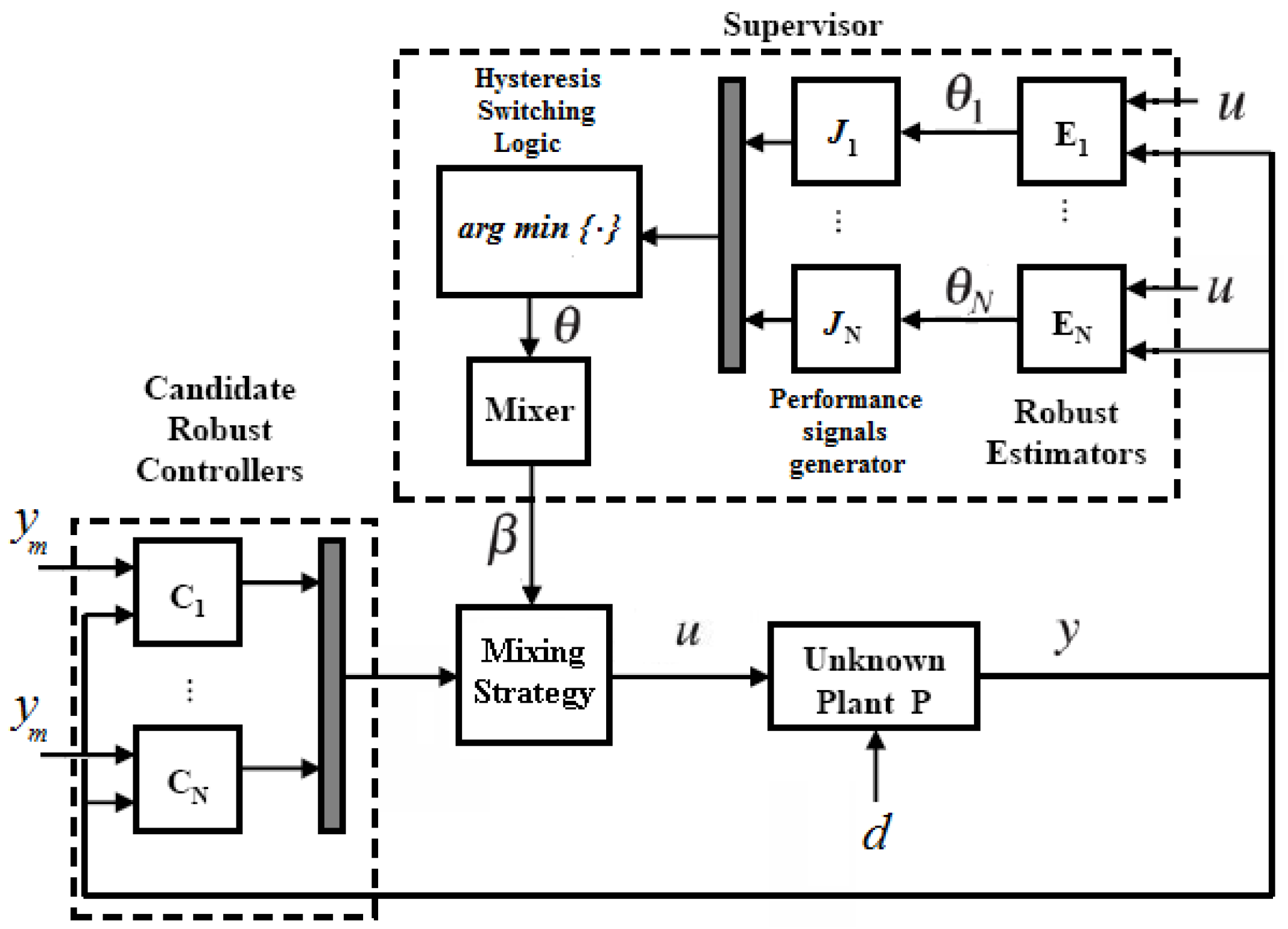
The structure of the Multi-AMC is shown in Figure 1. The novelty of the new architecture is the combination of the controller mixing with multiple parameter estimators. The supervisor comprises of various subsystems: the parallel on-line parameter estimators generate real-time estimates , of the unknown parameter vector . The switching logic, using performance signals based on the past and present estimation error, orchestrates the decision of the best estimate among all parallel parameter estimates at each time t. Finally, the mixer determines the participation level of each candidate controller based on the selected estimate .
Figure 1.
Multi-AMC architecture.

The stability and stability robustness properties of the Multi-AMC scheme are described by the following Theorem.
Theorem 2 Let the unknown plant given by (1)–(3) satisfy the plant assumptions P1–P5. Consider the adaptive mixing controller with the multicontroller given by (6) and satisfying assumptions C1–C2; the mixer (7) satisfying M1; the parallel robust adaptive laws given by (8)–(11) and hysteresis switching logic (16) and (17). Then the following results hold:
- If , , then all the closed-loop signals are bounded, i.e., ϕ, u, ; furthermore as .
- If , , then there exists such that, if where , is the system norm defined as , and a finite constant, then the adaptive mixing control scheme guarantees ϕ, u, y, andwhere , and .
Proof - Due to the modularity of the proposed approach, the proof can be lead by following analogous steps of the stability proof of the AMC scheme with a single estimator, which can be found in [12].
Remark 1 The stability and robustness results are conceptually similar to those in robust adaptive control [9,10,18]. The advantage of AMC in comparison with conventional robust adaptive control is that for the proposed scheme the stabilizability of the estimated plant is no longer an issue in calculating on-line the controller parameters. In addition, it allows well developed results from robust control to be incorporated in the design. In fact, thanks to the modularity of the design, the analysis of the overall system relies on certain properties of its individual parts. Furthermore, the Multi-AMC can handle controllers that are not directly parameterized by the unknown plant parameters, e.g., or μ-synthesized robust controllers, extending the class of feedback adaptive control systems.
Remark 2 Equation (19) is a mean square condition: it does not guarantee that the tracking error will be bounded from above by the modeling error bound at all times. As in conventional adaptive control, a phenomenon known as “bursting” [19], where the tracking error assumes large values over short intervals of time, cannot be excluded by the mean square bound. One way to get rid of bursting is to use a dead zone to switch-off adaptation when convergence to steady state values is achieved [20].
6. Numerical Example
Despite the results of Theorem 2, establishing analytically that the Multi-AMC scheme will guarantee better transient performance than other adaptive schemes is difficult if at all possible. Transient performance can be just numerically demonstrated via extensive simulations. This section is devoted to simulation testing of the proposed Multi-AMC scheme.
The numerical example used for simulations is a two carts system, shown in Figure 2, composed of two masses moving on a horizontal plane with known dynamic friction coefficient . The two carts are coupled with a spring, producing an elastic force proportional to its deformation through an unknown stiffness constant . In the simulations reported hereafter we consider and . Though apparently academic, this numerical example has been widely studied, since the two carts structure appears in many vibration suppression problems and in control of flexible structures.
Figure 2.
The two-carts benchmark example.
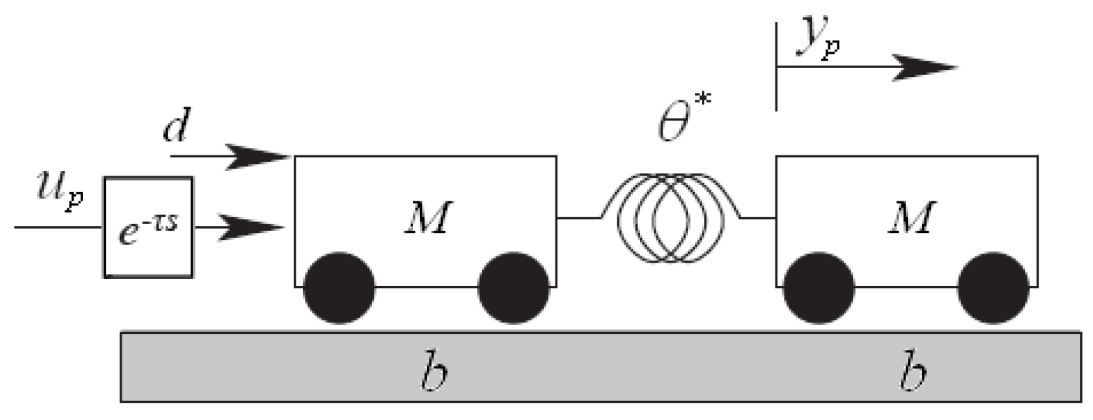
The measurement available is the second cart displacement. The control is applied to the first cart through a control channel with a time delay of , which represents the unmodeled dynamics. The control objective is to control the position of the second cart applying a force to the first cart. The plant input is corrupted with an additive zero mean white actuator noise , parallel to the track, with variance , and chopped between in order to obtain a bounded noise. The reference to be tracked is a square-wave of amplitude between 0 and 1 and with period . The continuous-time model is discretized using Euler’s approximation of the derivative with sampling time as in [21]. The nominal discrete-time plant is given by:
where , , . The unknown constant stiffness is restricted to the compact set
We consider the family of candidate controllers , designed on nominal models with stiffness , , , , , , , respectively. The controller synthesis has been performed using a weighted mixed-sensitivity criterion [22], as described in [23], and discretizing the resulting controllers with sampling time .
The coefficients of and are reported in Table 1, together with their corresponding stability intervals , which is the sets of plants with stiffness that are stabilized by the controller , i.e.,

| 146.257 | −428.616 | 419.360 | −136.999 | −2.464 | 2.038 | −0.563 | ||
| 79.779 | −233.668 | 228.558 | −74.668 | −2.457 | 2.026 | −0.559 | ||
| 43.739 | −128.102 | 125.361 | −40.997 | −2.446 | 2.010 | −0.553 | ||
| 31.680 | −92.798 | 90.877 | −29.757 | −2.435 | 1.994 | −0.547 | ||
| 22.632 | −66.341 | 65.092 | −21.380 | −2.411 | 1.958 | −0.533 | ||
| 19.309 | −56.746 | 56.013 | −18.571 | −2.323 | 1.830 | −0.485 | ||
| 17.744 | −54.669 | 57.372 | −20.436 | −1.865 | 1.187 | −0.252 |
The mixer is constructed on the basis of the smooth bump function if , and otherwise. Because of the scalar nature of the uncertainty set, consider the pre-normalized weights,
where and are the upper and lower bound, respectively, of the subset . The mixing signal is generated by normalizing , i.e.,
The parameter subsets , , are:
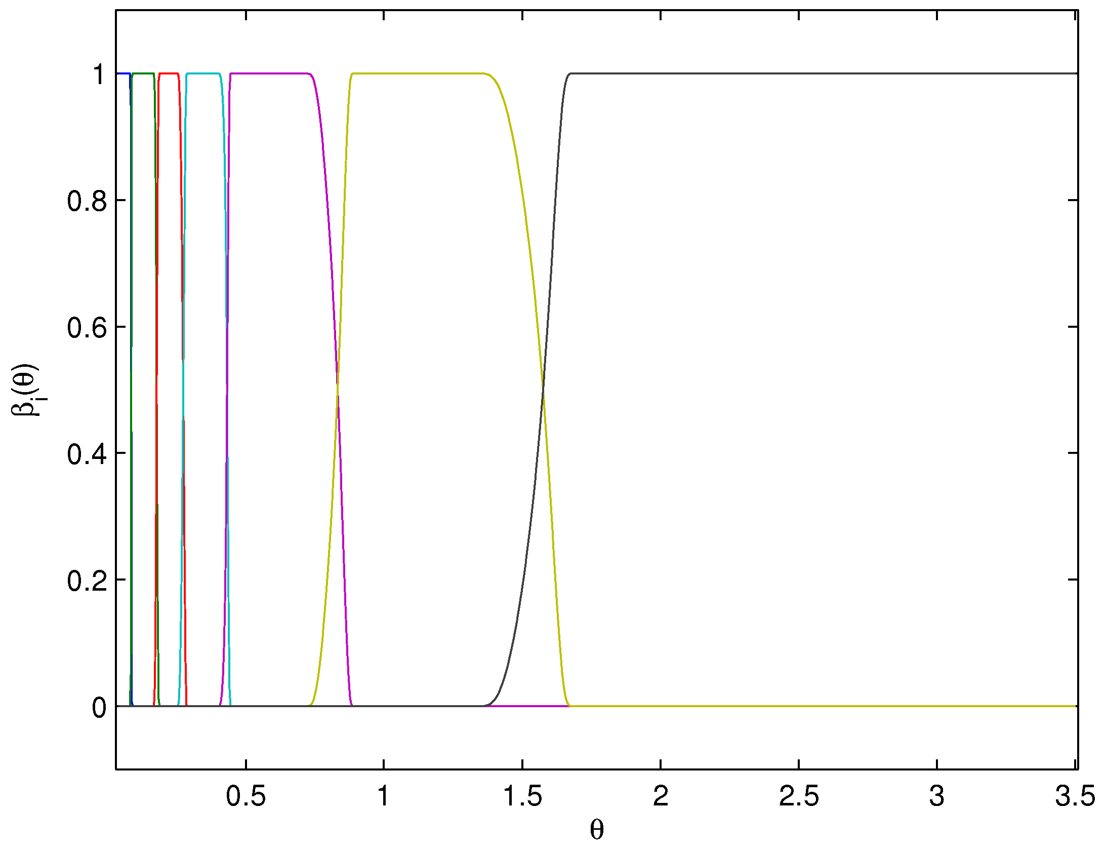
The subsets have been found by a trial and error procedure, taking into account the stability intervals in Table 1. Note that the plant is harder to control as the uncertain stiffness is small. This is reflected by the stability intervals of each controller, which are not equally distributed over the whole uncertainty set: in particular, in the interval one controller is sufficient to control the plant, while in the interval six controllers are needed. The mixing function derived from the described procedure is shown in Figure 3. The multicontroller has been constructed using output blending, i.e., , since this approach has been verified to satisfy assumption C2.
Figure 3.
Mixing strategy: , .

The design parameters of the robust adaptive laws and of the hysteresis logic have been chosen as follows:
The initial condition for each estimator has been chosen as the middle point of the subset .
The Multi-AMC is compared with the AMC scheme that uses a single parameter estimator [11], with the same design parameters as the parallel adaptive laws, and initial condition , which is the center of the overall parameter interval Ω. For a comparison with a conventional adaptive controller, a discrete-time pole-placement adaptive controller (APPC) is implemented, using the same single adaptive law as in the single estimator based AMC scheme. The pole-placement is designed to place the closed-loop poles at the roots of , which is the characteristic polynomial of the fifth nominal model in feedback with the fifth candidate controller.
We compare the learning performance of the three approaches for the seven nominal values of the uncertain parameter, , , , , , and . We do not consider stiffness values up to , because one single controller is sufficient to take care of the uncertainty subset . Non-zero random initial conditions are assumed for the plant state (initial position and velocity of the 2 carts). For each nominal value of the uncertain parameter we run 20 Monte Carlo simulations: each simulation has a time-length of . The criteria used to evaluate the performance of each scheme are:
- The root mean square (RMS) tracking error over the first 50 seconds. This criterion is used to evaluate transient and tracking error performance.
- The average time it takes for the scheme to converge to the final controller without any further switching (used in the comparison of the single estimator based AMC with the Multi-AMC).
The results are given in Table 2 for the ideal case (, ) and in Table 3 for the noisy case with unmodeled dynamics (). A consistent tracking error RMS improvement of the Multi-AMC scheme can be seen with respect to both the APPC scheme and the AMC with a single estimator. The column next to the tracking error RMS values evaluates the percentage RMS improvement of the Multi-AMC over the other two schemes. As expected, the RMS improvements are more drastic when the initial parameter estimate is further away from the true unknown parameter. There is no improvement between Multi-AMC and AMC in the case , because both approaches start with an initial parameter estimate corresponding to the selection of the stabilizing candidate controller without subsequent switching.
The second performance criterion, shown in the last two columns of Table 2 and Table 3, is the mean time, calculated among all the simulations, after which, for both AMC schemes, the weight associated to the final selected controller remains in the interval . Thanks to the discontinuous adaptation orchestrated by the switching logic, the Multi-AMC convergence to the final controller is faster than the AMC employing a single estimator, as demonstrated in the last column of Table 2 and Table 3.
| Tracking error RMS | Multi-AMC RMS Improvement | Convergence to final controller | ||
|---|---|---|---|---|
| Multi-AMC | 2.395 | 7.5 sec. | ||
| AMC | 0.05 | 6.567 | 63.5 % | 22.0 sec. |
| APPC | 20.393 | 88.3 % | ||
| Multi-AMC | 1.852 | 7.1 sec. | ||
| AMC | 0.1 | 4.331 | 57.2 % | 16.5 sec. |
| APPC | 15.488 | 88.0 % | ||
| Multi-AMC | 1.411 | 7.2 sec. | ||
| AMC | 0.2 | 3.120 | 54.8 % | 12.7 sec. |
| APPC | 11.721 | 88.0 % | ||
| Multi-AMC | 0.989 | 5.9 sec. | ||
| AMC | 0.3 | 1.815 | 45.5 % | 11.3 sec. |
| APPC | 6.816 | 85.5 % | ||
| Multi-AMC | 0.641 | 3.7 sec. | ||
| AMC | 0.5 | 1.045 | 38.7 % | 9.5 sec. |
| APPC | 3.304 | 80.6 % | ||
| Multi-AMC | 0.458 | 4.1 sec. | ||
| AMC | 1.0 | 0.606 | 24.4 % | 4.9 sec. |
| APPC | 1.164 | 60.7 % | ||
| Multi-AMC | 0.584 | 0 sec. | ||
| AMC | 2.0 | 0.584 | 0 % | 0 sec. |
| APPC | 0.761 | 22.7 % |
| Tracking error RMS | Multi-AMC RMS Improvement | Convergence to final controller | ||
|---|---|---|---|---|
| Multi-AMC | 1.881 | 7.0 sec. | ||
| AMC | 0.05 | 4.390 | 57.2 % | 22.9 sec. |
| APPC | 15.215 | 87.6 % | ||
| Multi-AMC | 1.746 | 7.0 sec. | ||
| AMC | 0.1 | 3.927 | 55.5 % | 13.8 sec. |
| APPC | 14.047 | 87.6 % | ||
| Multi-AMC | 1.669 | 7.2 sec. | ||
| AMC | 0.2 | 3.192 | 47.7 % | 12.8 sec. |
| APPC | 11.939 | 86.0 % | ||
| Multi-AMC | 1.340 | 5.1 sec. | ||
| AMC | 0.3 | 2.083 | 35.7 % | 12.7 sec. |
| APPC | 7.739 | 82.7 % | ||
| Multi-AMC | 0.744 | 4.6 sec. | ||
| AMC | 0.5 | 1.014 | 26.6 % | 10.3 sec. |
| APPC | 3.890 | 80.9 % | ||
| Multi-AMC | 0.508 | 4.2 sec. | ||
| AMC | 1.0 | 0.619 | 17.9 % | 4.8 sec. |
| APPC | 1.415 | 64.1 % | ||
| Multi-AMC | 0.586 | 0 sec. | ||
| AMC | 2.0 | 0.586 | 0 % | 0 sec. |
| APPC | 0.803 | 27.0 % |
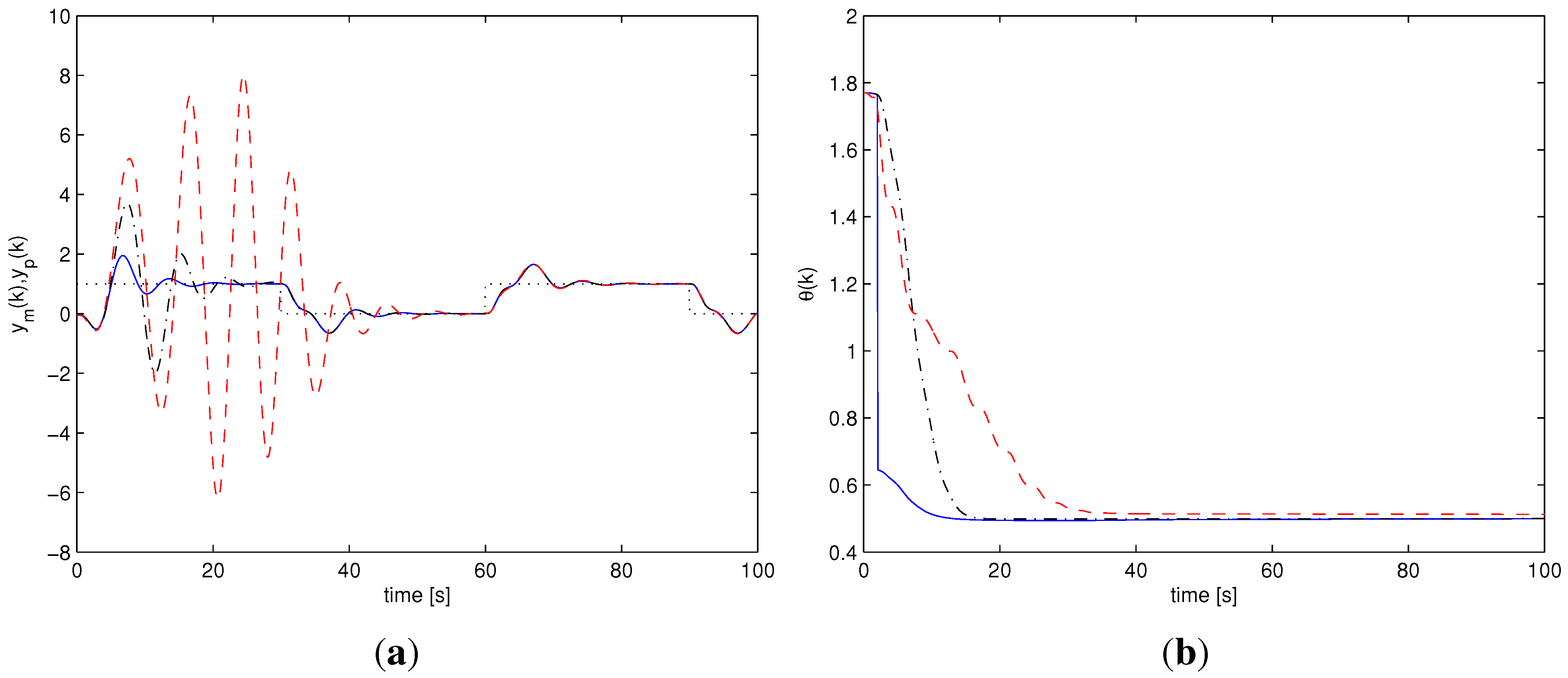
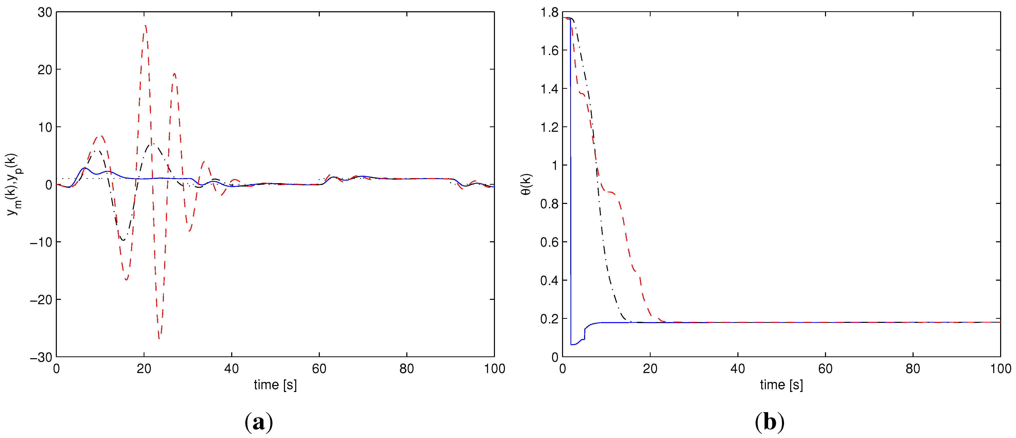
Among all the performed simulations, two particular scenarios have been chosen to graphically show and compare the behavior of the different adaptive schemes. One scenario does not involve noise or unmodeled dynamics, with a value of the uncertain stiffness corresponding to . The other scenario considers the noisy situation with unmodeled delay , with uncertain stiffness .
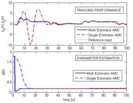
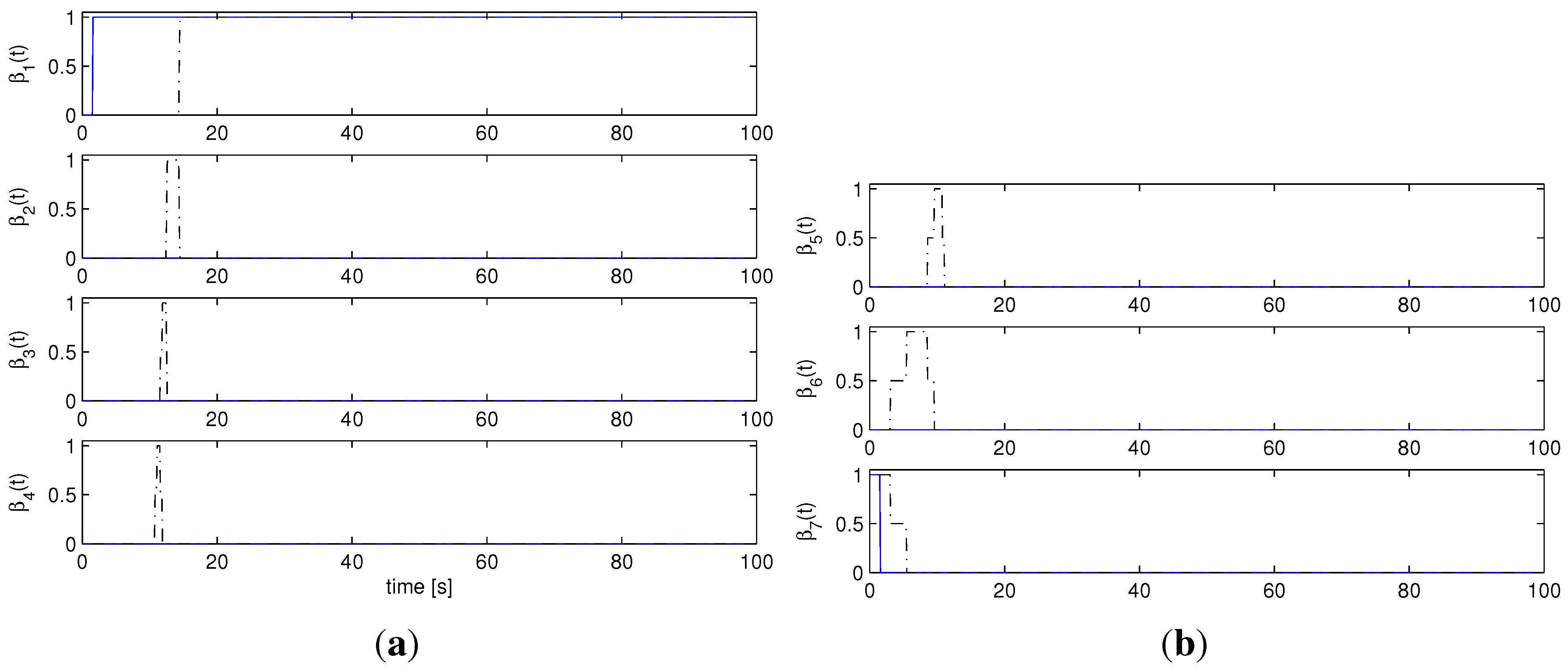
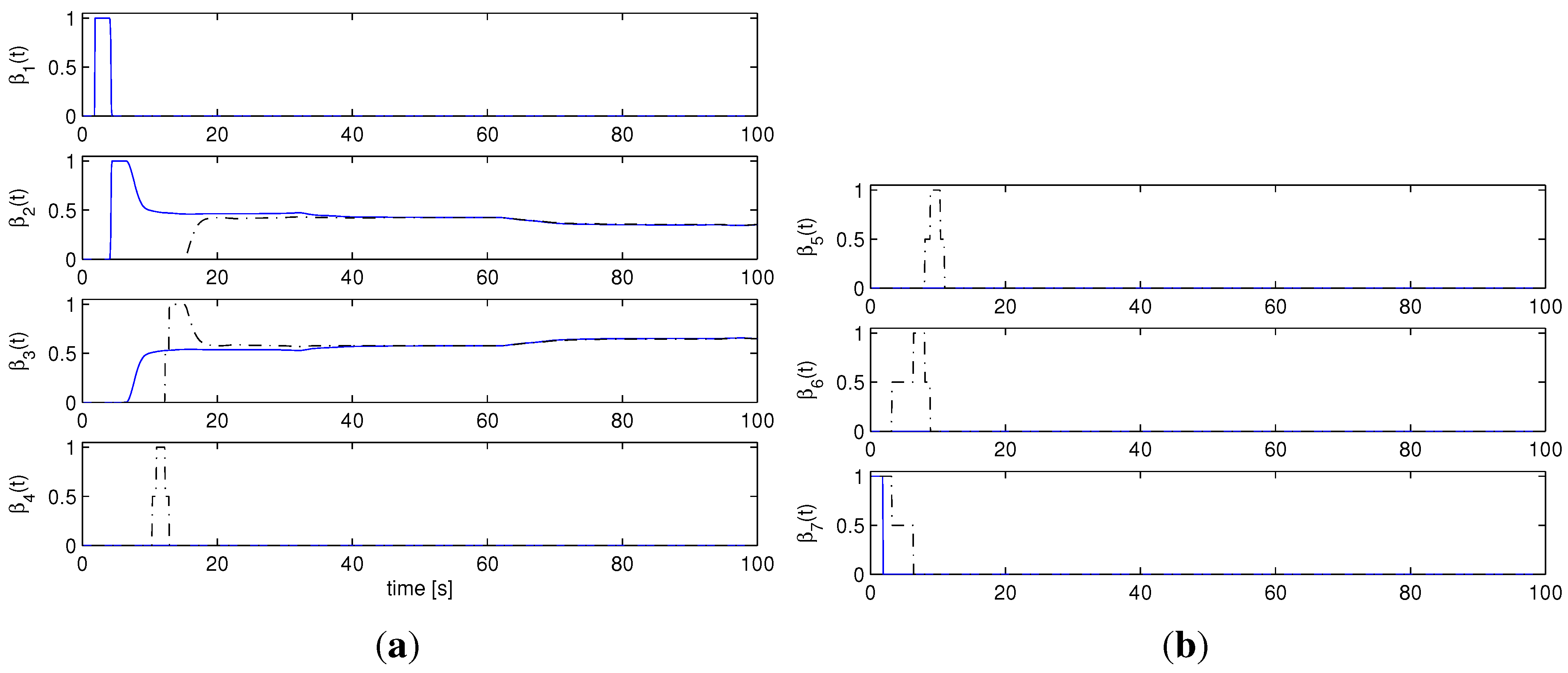
Figure 4(a) and Figure 5(a) show the output responses for the three adaptive schemes, for the two scenarios. In Figure 4(b) and Figure 5(b) the evolution of the parameter estimate is shown. Figure 6(a), Figure 6(b), Figure 7(a) and Figure 7(b) show the AMC mixer weights. In both cases it is possible to see that the Multi-AMC scheme exhibits a smaller transient when compared with both the APPC scheme and the single estimator AMC scheme. The Multi-AMC estimated parameter converges to the true value much faster that the other two schemes, which reflects a faster convergence of the mixing weights to a stabilizing controller.
Figure 4.
Ideal case, : Multi-AMC (solid), AMC (dash-dotted), APPC (dashed). (a) output response : Multi-AMC (solid), AMC (dash-dotted), APPC (dashed); (b) Parameter estimate : Multi-AMC (solid), AMC (dash-dotted), APPC (dashed).
Figure 4.
Ideal case, : Multi-AMC (solid), AMC (dash-dotted), APPC (dashed). (a) output response : Multi-AMC (solid), AMC (dash-dotted), APPC (dashed); (b) Parameter estimate : Multi-AMC (solid), AMC (dash-dotted), APPC (dashed).
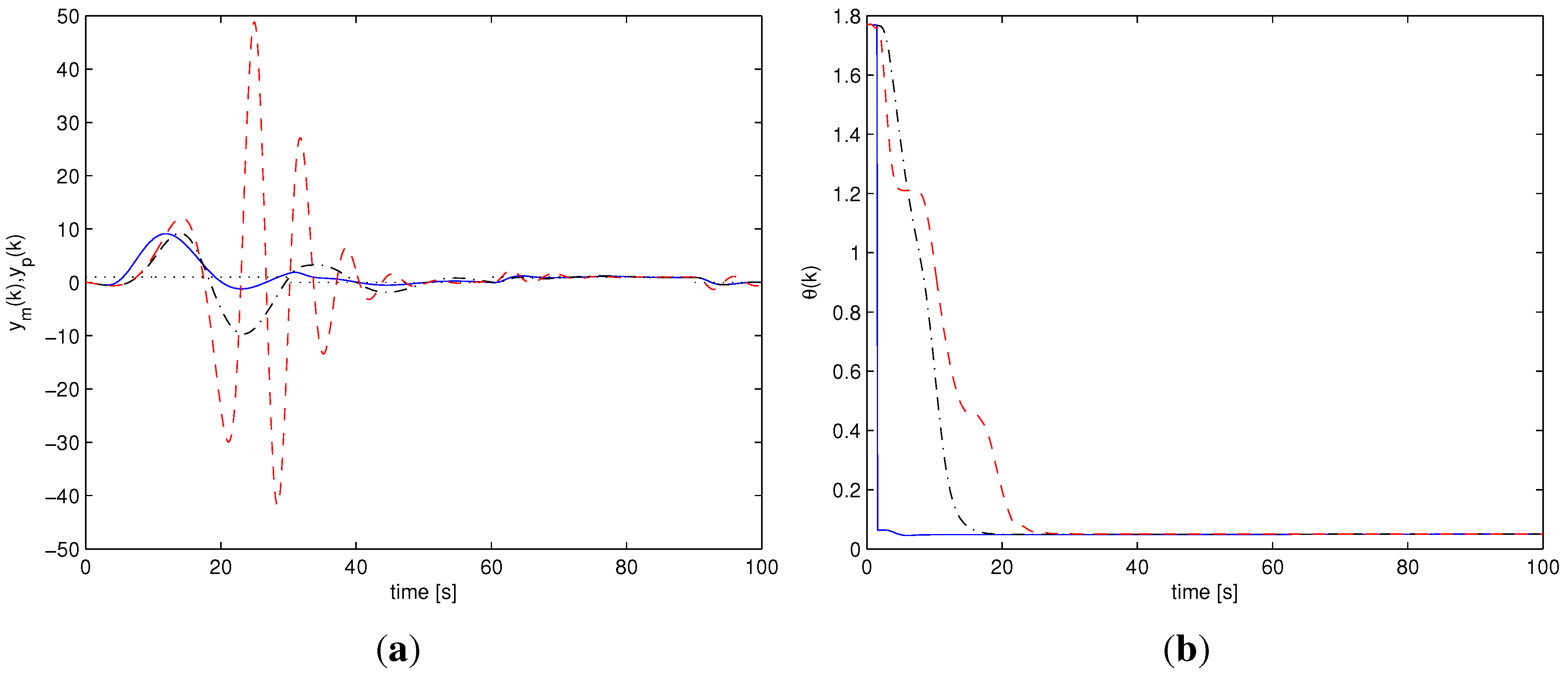
Figure 5.
Unmodeled dynamics, : Multi-AMC (solid), AMC (dash-dotted), APPC (dashed). (a) output response : Multi-AMC (solid), AMC (dash-dotted), APPC (dashed); (b) Parameter estimate : Multi-AMC (solid), AMC (dash-dotted), APPC (dashed).
Figure 5.
Unmodeled dynamics, : Multi-AMC (solid), AMC (dash-dotted), APPC (dashed). (a) output response : Multi-AMC (solid), AMC (dash-dotted), APPC (dashed); (b) Parameter estimate : Multi-AMC (solid), AMC (dash-dotted), APPC (dashed).

In order to clarify how the proposed adaptive method acts in the cases in which the unknown parameters belong to overlapping sets, one more scenario is shown, corresponding to with input noise and unmodeled delay (Figure 8(a)). Such scenario as well as other stiffness values belonging to overlapping sets are not shown in Table 2 and Table 3 both for the sake of compactness of the tables and because the transient results are similar to the results shown for the seven nominal values of the uncertain parameter. In Figure 8(b) the evolution of the parameter estimate is shown. Figure 9(a) and Figure 9(b) show the AMC mixer weights. Since belongs to both and , both controllers and run together in the loop (, ), thus leading to a blended control signal.
Figure 6.
Ideal case, : AMC controller weights : Multi-AMC (solid), AMC (dash-dotted). (a) , , , ; (b) , , .
Figure 6.
Ideal case, : AMC controller weights : Multi-AMC (solid), AMC (dash-dotted). (a) , , , ; (b) , , .

Figure 7.
Unmodeled dynamics, : AMC controller weights : Multi-AMC (solid), AMC (dash-dotted). (Note that, for both schemes, all the controller weights from to are zero for all ). (a) , , , ; (b) , , .
Figure 7.
Unmodeled dynamics, : AMC controller weights : Multi-AMC (solid), AMC (dash-dotted). (Note that, for both schemes, all the controller weights from to are zero for all ). (a) , , , ; (b) , , .
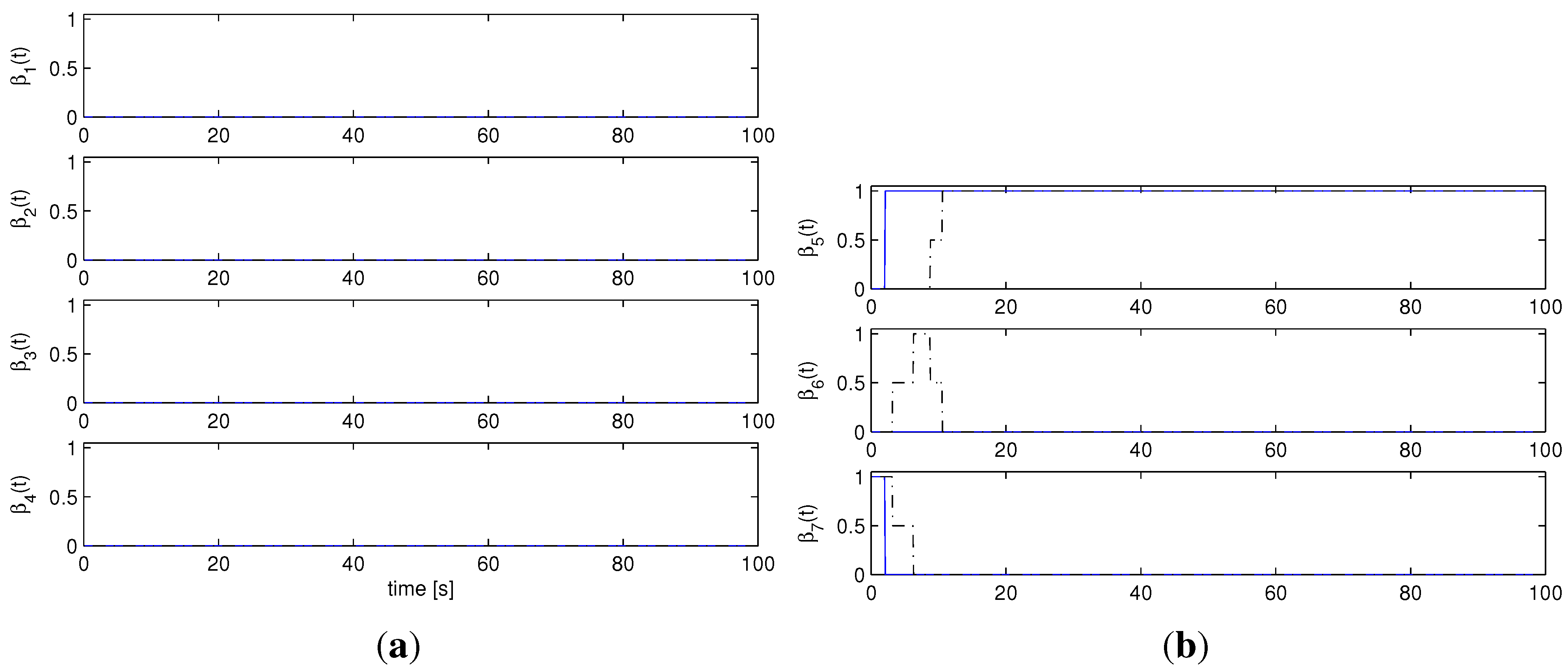
Figure 8.
Unmodeled dynamics, : Multi-AMC (solid), AMC (dash-dotted), APPC (dashed). (a) output response : Multi-AMC (solid), AMC (dash-dotted), APPC (dashed); (b) Parameter estimate : Multi-AMC (solid), AMC (dash-dotted), APPC (dashed).
Figure 8.
Unmodeled dynamics, : Multi-AMC (solid), AMC (dash-dotted), APPC (dashed). (a) output response : Multi-AMC (solid), AMC (dash-dotted), APPC (dashed); (b) Parameter estimate : Multi-AMC (solid), AMC (dash-dotted), APPC (dashed).

Figure 9.
Unmodeled dynamics, : AMC controller weights : Multi-AMC (solid), AMC (dash-dotted). (a) , , , ; (b) , , .
Figure 9.
Unmodeled dynamics, : AMC controller weights : Multi-AMC (solid), AMC (dash-dotted). (a) , , , ; (b) , , .
7. Conclusions
A new multiple model adaptive mixing control scheme employing a bank of parallel parameter estimators has been developed. The stability properties of the resulting architecture, namely (Multi-AMC), are analyzed (convergence of the tracking error to zero for the nominal and noiseless case, and bounded closed-loop states with tracking error of the order of the modeling error in the presence of unmodeled dynamics and bounded disturbances). The control scheme and the stability results have been carried out in discrete-time, for an easier implementation of the adaptive scheme in digital control. The proposed scheme achieves faster learning and better transient performance. A two carts system was used to demonstrate, via Monte Carlo simulations, the effectiveness of the proposed Multi-AMC in consistently improving the transient behavior when compared with standard adaptive pole placement and a single estimator AMC scheme.
Appendix: Proof of Theorem 1
The conditions A1 and A2 of the HSL Lemma are satisfied in the ideal case with no unmodeled dynamics and disturbances, using the performance signals (14). In fact, the functionals (14) are monotone non-decreasing, so they have a limit (which may be infinite). Besides, since for some index j, there is always at least one estimator such that , which implies is bounded. Hence, there is a finite time , after which no more switching occurs and, moreover, is bounded. The conclusion is that, because of the final switching time and the boundedness of the final test functional, it is possible to show that , , . From (thanks to parameter projection) and , we have , , which is property E1.
When unmodeled dynamics and disturbances are present, in order to satisfy conditions A1–A2 of the HSL Lemma, the performance signals (15) must be used in the switching logic. In this case, thanks to the max operator, the functionals (15) are monotone non-decreasing, so they have a limit (which may be infinite). Besides, since for some index j, there is always at least one estimator such that , . Note that the boundedness in the mean square sense of implies the boundedness of the functional in (15). Hence, there is always an index j such that is bounded. Using the HSL Lemma it follows that there is a finite time , after which no more switching occurs and, moreover, is bounded. The conclusion is that , , which is property E2.
References
- Morse, A.S. Supervisory control of families of linear set-point controllers, part 1: Exact matching. IEEE Trans. Autom. Control 1996, 41, 1413–1431. [Google Scholar] [CrossRef]
- Narendra, K.; Balakrishnan, J. Adaptive control using multiple models. IEEE Trans. Autom. Control 1997, 42, 171–187. [Google Scholar] [CrossRef]
- Hespanha, J.P.; Liberzon, D.; Morse, A.S. Hysteresis-based switching algorithms for supervisory control of uncertain systems. Automatica 2003, 39, 263–272. [Google Scholar] [CrossRef]
- Liberzon, D. Switching in Systems and Control; Birkhӓuser: Basel, Switzerland, 2003. [Google Scholar]
- Fekri, S.; Athans, M.; Pascoal, A. Issues, progress and new results in robust adaptive control. Int. J. Adapt. Control Signal Process. 2006, 20, 519–579. [Google Scholar] [CrossRef]
- Stefanovic, M.; Safonov, M.G. Safe adaptive switching control: Stability and convergence. IEEE Trans. Autom. Control 2008, 53, 2012–2021. [Google Scholar] [CrossRef]
- Rosa, P.; Silvestre, C.; Shamma, J.S.; Athans, M. Multiple-model Adaptive Control with Set-valued Observers. In Proceedings of the 48th IEEE Conference on Decision and Control, Shanghai, China, 16–18 December 2009.
- Baldi, S.; Battistelli, G.; Mosca, E.; Tesi, P. Multi-model unfalsified adaptive switching supervisory control. Automatica 2010, 46, 249–259. [Google Scholar] [CrossRef]
- Ioannou, P.A.; Sun, J. Robust Adaptive Control; Prentice Hall: Upper Saddle River, NJ, USA, 1996. [Google Scholar]
- Tao, G. Adaptive Control: Design and Analysis; John Wiley & Sons: Hoboken, NJ, USA, 2003. [Google Scholar]
- Kuipers, M.; Ioannou, P.A. Multiple model adaptive control with mixing. IEEE Trans. Autom. Control 2010, 55, 1822–1836. [Google Scholar] [CrossRef]
- Baldi, S.; Ioannou, P.A.; Mosca, E. Multiple model adaptive control with mixing: The Discrete-time case. IEEE Trans. Autom. Control 2012, 57, 1040–1045. [Google Scholar] [CrossRef]
- Nichols, R.A.; Reichert, R.T.; Rugh, W.J. Gain scheduling for H-infinity controllers: A flight control example. IEEE Trans. Control Syst. Technol. 1993, 1, 69–79. [Google Scholar] [CrossRef]
- Reichert, R. Dynamic scheduling of modern-robust control autopilot designs for missiles. IEEE Control Syst. Mag. 1992, 12, 35–42. [Google Scholar] [CrossRef]
- Stilwell, D.J.; Rugh, W.J. Stability preserving interpolation methods for the synthesis of gain scheduled controllers. Automatica 2000, 36, 665–671. [Google Scholar] [CrossRef]
- Baldi, S.; Ioannou, P.A.; Mosca, E. Discrete-time Adaptive Mixing Control with Stability-preserving Interpolation: The Output Regulation Problem. In Proceedings of the 18th IFAC World Congress, Milan, Italy, 28 August–2 September 2011.
- Morse, A.S.; Mayne, D.Q.; Goodwin, G.C. Applications of hysteresis switching in parameter adaptive control. IEEE Trans. Autom. Control 1992, 37, 1343–1354. [Google Scholar] [CrossRef]
- Ioannou, P.A.; Fidan, B. Adaptive Control Tutorial; Advances in design and control, SIAM: Philadelphia, PA, USA, 2006. [Google Scholar]
- Anderson, B. Adaptive systems, lack of persistency of excitation and bursting phenomena. Automatica 1985, 21, 247–258. [Google Scholar] [CrossRef]
- Tsakalis, K.; Ioannou, P. Linear Time Varying Systems: Control and Adaptation; Prentice Hall: Englewood Cliffs, NJ, USA, 1993. [Google Scholar]
- Angeli, D.; Mosca, E. Lyapunov-based switching supervisory control of nonlinear uncertain systems. IEEE Trans. Autom. Control 2002, 47, 500–505. [Google Scholar] [CrossRef]
- Kwakernaak, H. The Polynomial Approach to Optimal Regulation. In Control Theory, Lecture Notes in Mathematics; Mosca, E., Pandolfi, L., Eds.; Springer: Berlin, Germany, 1991; Volume 1496, pp. 141–221. [Google Scholar]
- Mosca, E.; Agnoloni, T. Inference of candidate loop performance and data filtering for switching supervisory control. Automatica 2001, 37, 527–534. [Google Scholar] [CrossRef]
- *This work has been supported by the European Commission FP7-ICT-5-3.5, Engineering of Networked Monitoring and Control Systems, under the contract #257806 AGILE.
© 2013 by the author; licensee MDPI, Basel, Switzerland. This article is an open access article distributed under the terms and conditions of the Creative Commons Attribution license (http://creativecommons.org/licenses/by/3.0/).
Share and Cite
MDPI and ACS Style
Baldi, S. Multiple Estimation Architecture in Discrete-Time Adaptive Mixing Control. Machines 2013, 1, 33-49. https://doi.org/10.3390/machines1010033
AMA Style
Baldi S. Multiple Estimation Architecture in Discrete-Time Adaptive Mixing Control. Machines. 2013; 1(1):33-49. https://doi.org/10.3390/machines1010033
Chicago/Turabian StyleBaldi, Simone. 2013. "Multiple Estimation Architecture in Discrete-Time Adaptive Mixing Control" Machines 1, no. 1: 33-49. https://doi.org/10.3390/machines1010033