1. Introduction
Downtime due to errors is costly in flexible manufacturing systems [
1,
2]. It is therefore desirable to perform a quick and correct recovery in order to resume the nominal production after an error. Among others, [
3,
4] see automatic error recovery as a must in todays manufacturing systems.
Error recovery in complex systems is a complicated task [
5], often divided into three major activities [
6]:
detection of discrepancies between the intended behavior and the actual behavior of a system,
diagnosis to find the original fault causing the observed error, and
recovery of the system to continue the nominal production. Recovery is further partitioned into
error correction and
restart. The error correction phase concerns the process to remove underlying faults and repair the resource(s) if required. The restart phase, which is the focus of this paper, then covers the process to resume the nominal production.
A wide variety of possible errors may cause failures in a manufacturing system. For example, a part may be missing in a resource, be badly positioned in a fixture, or be not enough processed. Resources may stop working due to faulty sensors and/or actuators, such as worn out cutting tools and broken weld guns. Typical manufacturing system errors are listed by [
7,
8,
9], among others.
Some errors may be foreseen and appropriate corrective actions may then be included in the control system, see for example [
6,
10,
11]. Tip-dressing of the electrodes used in weld applications is an example of a proactive corrective action to avoid a failure [
9].
In general, however, it is impossible to foresee all errors that may occur and/or include all corrective actions in the control system [
3]. Thus, restart after unforeseen errors is often not supported correctly or as efficiently as it should in relation to the potential cost of the resulting downtime.
The control system for a manufacturing system is often based on a set of
operations that are to be executed in order to refine a product [
12]. Each operation is typically modeled by three states; an
executing state that is preceded by a state to model that the operation has not yet started, and succeeded by a state to model that the operation is completed. Possible operation sequences emerge through
dependencies between the operations [
12].
The nominal production may then be viewed as a trajectory between a composed source state where none of the operations have started, to a composed target state where a subset of the operations have completed. Each control system state on the trajectory will then model that some operations have not started, some operations are executing, and that the rest of the operations have completed.
For the sake of control and supervision, the resources and the product(s) in the manufacturing system can be abstracted into a set of physical states. When an operation is executed, the manufacturing system will, typically, change between many physical states. Thus, several physical states correspond to each control system state. Moreover, during the nominal production, the control system state evolves in synchrony with the corresponding physical states.
An unforeseen error is then a physical state that does not correspond to the current active control system state. Moreover, the actions required when correcting the error may force an operator to further corrupt the physical state during the error correction phase, such as moving a robot to a home-state. Thus, it is reasonable to assume that the control system and the resources are unsynchronized after the correction phase [
13].
The aim of the restart phase is then to
resynchronize the control system and the resources [
9]. This may necessitate to update both the active state of the control system and the physical state of the manufacturing system.
As a consequence, the objective in most error recovery methods presented in the literature, is to restart the system such that the nominal production may continue from either an earlier, a later, or the current control system state with respect to the active control system state at the time of the error [
8,
14]. This state from where the control system is continued is often called a
restart state [
9]. Recovery in an earlier or a later state is often referred to as
backward and
forward error recovery, respectively. Flexible manufacturing systems enable, however, production according to multiple operation sequences [
12], so backward and forward error recovery are seldom well defined. Thus, the recovery concept must be generalized in order to handle flexible manufacturing systems with multiple operation sequences.
When recovering the control system from an earlier state, it may be necessary to reexecute some of the operations [
9,
13,
15]. However, the existence of a physical product will constrain the reexecution [
7,
9,
14,
16], certain
reexecution requirements must be satisfied. For instance, an operation to fixate a part may be reexecuted as long as the succeeding refinement operation has not been started. This is in contrast to a glue applying operation that typically cannot be reexecuted.
Many of the restart methods presented in the literature are tailor made for specific types of manufacturing systems. Body-in-white manufacturing systems in the automotive industry is the main application for the methods presented in [
5,
9,
15]. The method in [
17] focuses on error recovery connected to loading, processing, and unloading CNC machines. Error recovery for systems where a set of resources are linked with material handling devices and intermediate buffers are described in [
7]. A method that is suitable for, but not limited to, error recovery in batch systems is presented in [
18]. To increase the transparency, it would be beneficial with more general methods less biased towards any specific type of system.
Few of the restart methods presented in the literature give a clear insight for how to systematically implement the theoretical ideas into a general control system for an industrial manufacturing system; among the exceptions are [
4,
5,
19]. Some methods require a specific control system architecture and are hence not generally applicable, see for example [
13,
15,
20].
Overviews of different techniques used in restart methods are given in [
6,
9,
18]. In [
9], some restart methods are also classified according to if the main work load is
online when an error has been diagnosed, or
offline before start of production.
Online methods, such as [
4,
7,
8,
16,
17,
18,
19,
20,
21], typically gather a majority of the relevant restart information at the time of the error and then perform backward or forward error recovery [
8]. Some methods, [
16,
19], reschedule the operations in the control system to find a new operation sequence after the error. A method that dynamically disables events in the control system when an error is detected is presented in [
4]. Most industrial control systems are, however, not powerful enough for methods that require heavy calculation online, so such approaches contradict the industrial desire to keep the online control system simple [
9].
Methods where the main work is done offline, such as [
1,
9,
10,
11,
13,
22,
23,
24,
25], have an advantage compared to online methods, not only due to the need of less powerful hardware online. Beforehand calculation enables different restart alternatives to be analyzed already when the production in the manufacturing system is planned, such that undesirable situations can be resolved if possible. This beforehand analysis is a big advantage for the offline methods.
Motivated by the existing methods and their limitations, this paper presents an offline method for calculating restart states. The proposed method is neither tailor made for, nor limited to a specific type of manufacturing system or control system. The overall idea of the proposed method is related to the method presented in [
5,
9], but with some major generalizations, that will be clearly pointed out in the remainder of this section.
As for all offline methods, it is assumed that the restart consists of an
offline phase, where the restart states are calculated, and an
online phase, where these states are used when the manufacturing system is to be restarted after an error. As in [
13] it is assumed that an error can only occur when one or more of the resources are used. In order to relate control system states on different operation sequences, the proposed method introduces the concept of
upstream states which generalizes the concept of backward error recovery.
To benefit from existing advances using formal methods, the proposed method is based on the supervisory control theory [
26]. During an initial formalization part a user-given set of operations, with dependencies and reexecution requirements, are automatically translated into automata. The automata are automatically extended with transitions to model restart in all upstream states for each control system state where it is assumed that an error can occur. The proposed method enables alternative operation sequences and restart of multiple resources, and is not limited to straight sequences nor to restart of a single resource as in [
5].
Not all upstream states are, however, valid as restart states due to the dependencies and the reexecution requirements. Therefore, a supervisor [
26] is synthesized for the automata and the valid restart states are derived from this supervisor. Any supervisor synthesis algorithm can be used and not just a modified monolithic synthesis algorithm as in [
5]. Thus, more efficient algorithms such as compositional synthesis [
27] and/or symbolic synthesis [
28] can be used.
When restarting the control system from a valid restart state the nominal production can start immediately, no reduced start-up pace is required as in [
5]. Moreover, the restart states are connected to the control system states and not to the specific errors that have been detected. Thus, the method can handle restart after unforeseen errors.
With the restart states precalculated, the online restart phase is reduced to four straightforward steps. First, the operator selects a restart state from the precalculated ones, which can for example be stored in a database connected to the control system. Second, the active state of the control system is updated to the selected restart state. Thus, it is assumed that a mechanism for state transition is available in the control system. Third, the operator places the manufacturing system in a physical state corresponding to the selected restart state; the operator is beneficially guided by instructions for how to reach this physical state. Finally, the nominal production can be (re)started by the operator.
To simplify for an operator during the third step, when placing the manufacturing system in a physical state, the calculated restart states may be filtered. This paper shows filtering of restart states based on physical states in the manufacturing system that are easily accessible, and the restart states that minimize the number of resources to be placed during the restart phase.
In addition, it is shown how to
adapt the nominal production to always enable desirable restart states, if there is at least one operation sequence in the system where the desired state is valid. This is accomplished by the uncontrollability property of the supervisory control theory [
26].
The paper is organized as follows. Preliminaries are given in
Section 2.
Section 3 introduces an example upon which the results are projected throughout the paper. General online error recovery with focus on the restart phase is discussed in
Section 4.
Section 5 will thereafter present how the calculation of restart states is formulated as a synthesis problem, without any reexecution requirements. Filtering of restart states is discussed in
Section 6. The reexecution requirements are then included in the calculation in
Section 7. How to adapt the nominal production to always enable desirable restart states is presented in
Section 8.
Section 9 gives some concluding remarks and future ideas.
2. Preliminaries
This section presents conventions and notations used in this paper. First, the modeling formalism is presented. Thereafter, this formalism is used to model the operations for a manufacturing system.
2.1. Automata and the Supervisory Control Theory
Definition 1 Finite automaton A finite automaton is a 5-tuple: where is the non-empty finite set of states; is the non-empty finite set of events (the alphabet); is the partial transition function; is the initial state; and is the set of marked states.
A transition is said to be fireable when the active state of the automaton A coincide with the source state q. When the transition is fired the active state of the automaton A is updated to the target state p. Let denote that an event e is defined from a state q in an automaton A. The active event function returns the set of events defined from a state q in A, .
The set of all finite sequences of events over an alphabet including the empty sequence, ε, is denoted . An element is called a string. For two strings and the concatenation is also in . The closure of a string s is denoted , such that . The transition function is extended to strings, such that , and . A state is then reachable in the automaton A if such that .
A language, denoted , is the set of strings generated from the initial state of the automaton A. Given an alphabet , represents the concatenation of all strings in with all events in . The marked language, , is the set of strings generated from the initial state reaching a marked state. The prefix closure of the marked language, denoted , is the set of all prefixes .
Interaction of two automata is modeled by full synchronous composition [
29].
Definition 2 Full synchronous composition (FSC) The full synchronous composition of two automata A and B is defined as where ; ; ; ; and
The
supervisory control theory (SCT) [
26] is a model-based framework for automatic calculation of discrete event controllers. Given a system to be controlled, a
plant P, and the intended behavior, a
specification , a
supervisor S may be synthesized, such that the behavior of
always fulfills
. In terms of languages
and
. The supervisor is both
non-blocking and
controllable [
26].
Non-blocking: The supervisor S guarantees that at least one marked state may be reached from every state in the system . This liveness property may formally be expressed as: .
Controllable: In SCT, a subset of the events is said to be uncontrollable. The supervisor S is never allowed to disable an uncontrollable event that might be generated by the plant P. With the assumption that , this safety property may formally be expressed as: .
Moreover, the supervisor is minimally restrictive, meaning that the plant is given the greatest amount of freedom to generate events without violating the specification. To facilitate the modeling, both the plant and the specification are often given as a set of automata that communicate through FSC. In the following, it is thus assumed that the system is modeled by several plants and specifications.
The focus of this paper is on calculating how a control system can be restarted. This problem is solved through synthesis of a supervisor and succeeding interpretation of the generated supervisor. Thus, any synthesis algorithm can be used to calculate the supervisor. In the following, the supervisor for
is assumed to be given as
, where
represents any synthesis algorithm. However, to facilitate the interpretation it is assumed that the supervisor is characterized through
guard extraction [
28].
In the guard extraction all controllable events are appended with a guard. Each guard is a boolean function that maps a state in to either true or false. A transition is said to be enabled by the supervisor if the guard for the labeling event is true in the source state of the transition.
Note that, the algorithm for guard extraction proposed in [
28] confronts the state-space explosion problem by using a symbolic representation of the full synchronous composition of the plants and the specifications. A user enters a set of automata and the supervisor is returned as a set of guards for the controllable events. Thus, guard extraction gives a concurrent model of modular automata.
A controllable event is termed an always enabled event if all transitions that are labeled by the event and having source states that are reachable in the supervised system are enabled by the supervisor. In contrast, the event is termed a sometimes enabled event if some but not all these transitions are enabled by the supervisor.
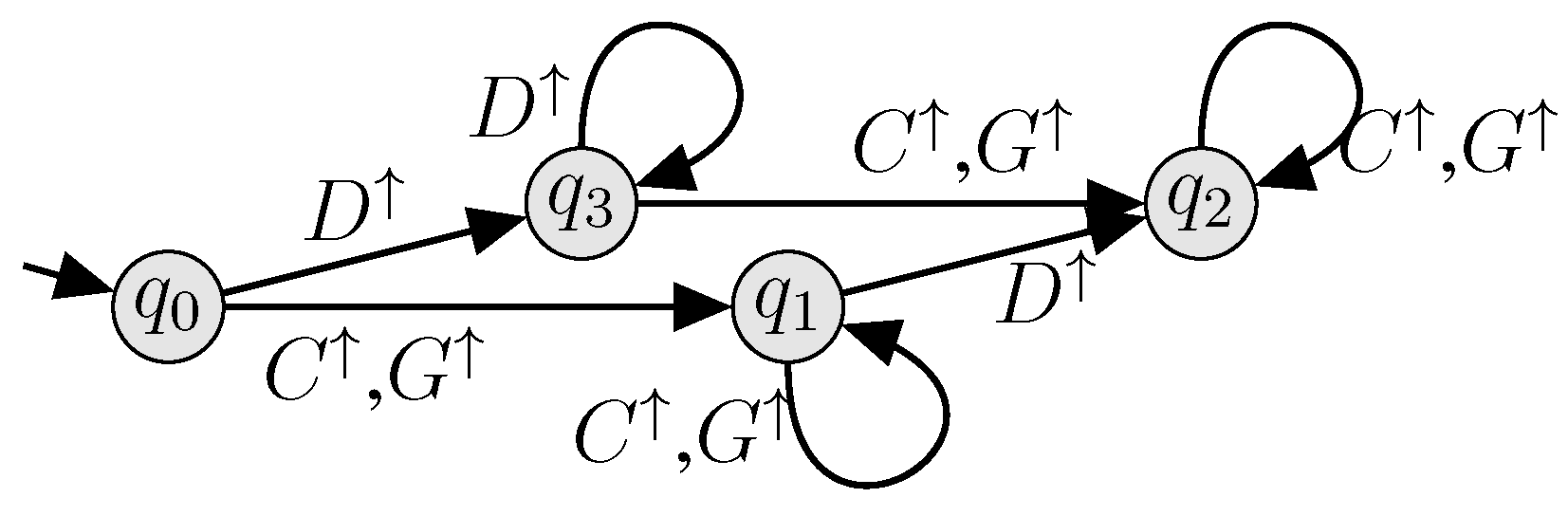
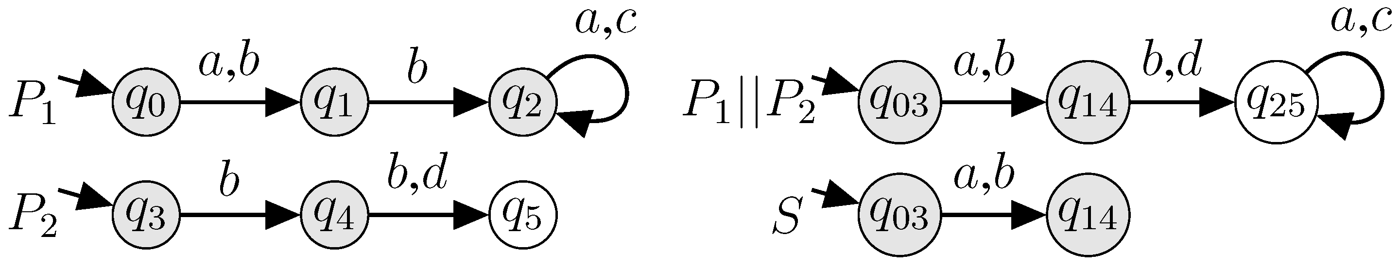
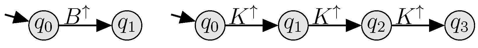
Guard extraction and the event terminology are exemplified on the supervisor for the two automata
and
in
Figure 1. Marked states are shaded in gray and all events are controllable. The automaton
is the FSC of
and
. Since the state
is blocking it is removed in the supervisor
. Thus, in
only the two transitions
and
are enabled by the supervisor.
Figure 1.
The events a and b are always and sometimes enabled events, respectively.
Figure 1.
The events a and b are always and sometimes enabled events, respectively.
In this example, the single always enabled event is a since one of the two transitions that are labeled by a in the FSC is enabled by the supervisor and the source state for the other transition is not reachable in the supervised system (the supervisor). The event b is sometimes enabled because only one of the two transitions having source states that are reachable in the supervised system and are labeled by b in the FSC is also enabled by the supervisor. The guard for b is not satisfied in the state . The disabled events c and d are neither always nor sometimes enabled.
Forbidden state combinations will be used in
Section 5 to model the (un-)desired behavior. In [
30] a method based on uncontrollability is presented for how to specify states locally in a set of automata such that the combination of these states are never reached in the supervised system. In the following, it is assumed that this or a similar method is used to encode given forbidden state combinations into the SCT framework.
2.2. Model of the System
In this paper, the control system for a manufacturing system is based on a set of operations, denoted Ω. These operations model the processes and tasks that are to be executed in order to refine a product. The basic assumption is that all operations are executed in parallel. This parallel execution of the operations can be restricted by dependencies.
The manufacturing system contains a set of resources, denoted . It is the resources that (physically) realize the operations. The resources required to realize an operation is denoted , such that .
To better understand how the different dependencies affect the relations between the operations, it is beneficial to visualize subsets of operations from Ω in different projections [
31]. Examples of such projections are the operations related to the main product flow or the operations realized by a specific resource. Throughout this paper, the graphical language
Sequences of Operations introduced in [
12] is used for the visualization of operations. Each visualization is referred to as a
sequence of operations (SOP).
An operation may formally be modeled by an automaton, a so called operation automaton.
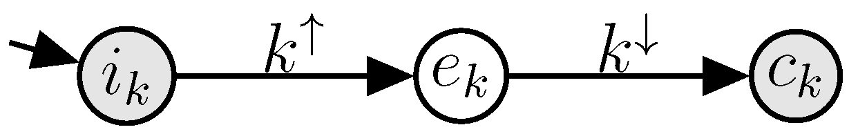
Definition 3 Operation automaton The automaton for an operation k is denoted where ; ; ; ; and .
The automaton
is illustrated in
Figure 2. The three states denote that the operation is initial (not started), executing, and completed, respectively. The two events in
are called
operation events.
Figure 2.
An operation k modeled by an automaton .
Figure 2.
An operation k modeled by an automaton .
Given the automaton for a single operation, the FSC of all automata for the operations in Ω can be defined. Note that, from a practical point of view an explicit representation of the complete state-space during synthesis is to be avoided.
Definition 4 FSC of operation automata The FSC of all automata for the operations in Ω is defined as: .
The operation progress for a system may then be given through the states in .
Definition 5 Operation progress For each state , three disjoint sets for the operation progress, the set of operations in their respective initial, executing, and completed state, denoted , , and , are defined as: The relation between an executing operation and the history of operation progress is captured by the definition of upstream states for an operation.
Definition 6 Upstream states for an operation Let be the set of states in where the operation k executes. For a state , a state is upstream of operation k if such that , and , and .
It follows from Definition 3 that each operation automaton contains a straight sequence of operation events and because the two states p and u must be connected through a string of operation events, all operations that are initial in the state p are initial in the upstream state u. With the same argument, the operations that are executing in p can either be initial or executing in u except for the operation k that is required to be initial in u. Moreover, the empty intersection in Definition 6 adds a requirement on the completed operations in p, they cannot be executing and must therefore be initial or completed in u.
3. Illustrating Example
Throughout this paper, the proposed method for calculating restart states is illustrated by the example introduced below.
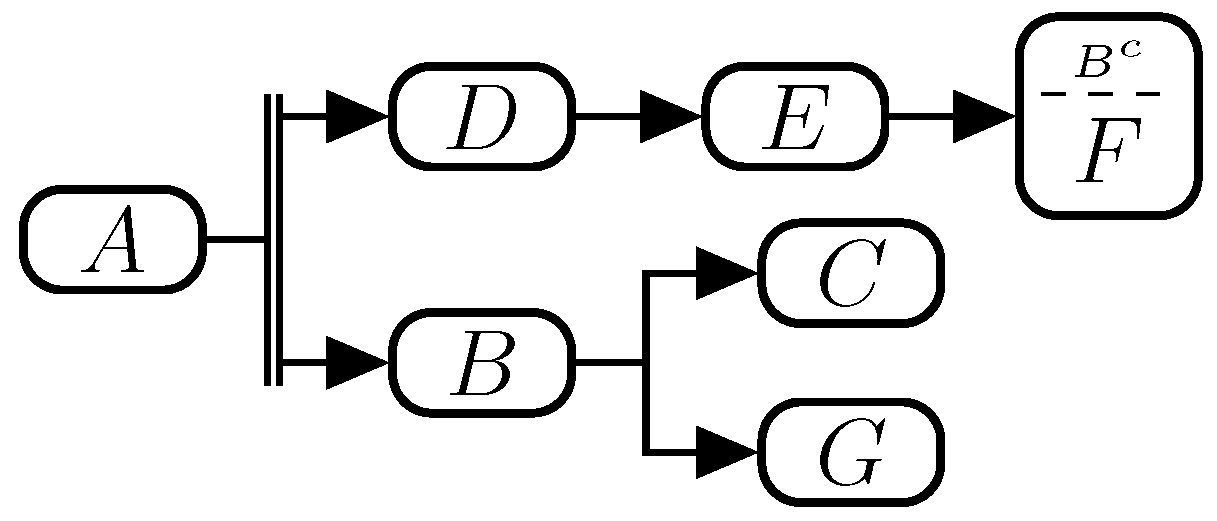
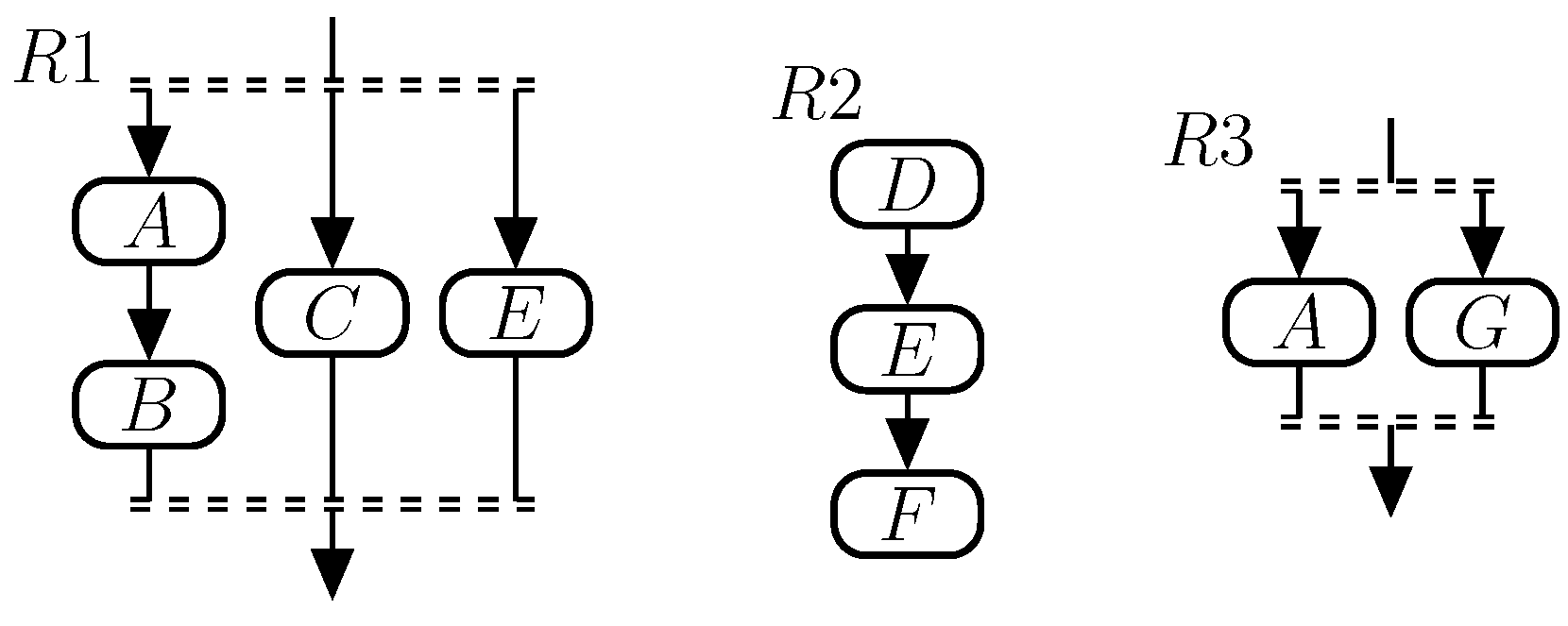
Example 1 A manufacturing system comprises three resources, , and its control system is modeled by seven operations, . The dependencies between the operations are visualized in different projections in the SOPs in Figure 3 and Figure 4. The three SOPs in Figure 4 show which resources that realize the different operations.
Figure 3.
Dependencies between the operations in Example 1.
Figure 3.
Dependencies between the operations in Example 1.
Figure 4.
Arbitrary order dependencies for resource allocation in Example 1.
Figure 4.
Arbitrary order dependencies for resource allocation in Example 1.
In the language Sequences of Operations, the dependencies between operations may be visualized both with expressions and graphical notations [
12]. An arrow visualizes a precedence dependency. As an example, operation
E cannot start before operation
D is completed. The expression
is also a visualization of a precedence dependency, that operation
F cannot start before operation
B is completed. The double bar visualizes that the two branches, starting with operations
D and
B, may execute in parallel, when operation
A is completed. An alternative dependency is visualized by a single bar, thus only one of the operations
C and
G may execute. The double dashed bars (see
Figure 4) visualize arbitrary order dependencies (mutual exclusion). All operations in each branch shall execute, but no branches execute in parallel.
Arbitrary order dependency is used to model resource allocation. Each resource can realize one operation at a time. Resource allocation and deallocation takes place in the first and in the last operation, respectively, in each branch. As an example, resource is allocated when the operations A, C, and E start and is thereafter deallocated when the operations B, C, and E complete. Thus, resource is allocated in the state where A is completed and B is initial.
5. To Calculate Restart States
This section presents how to offline calculate restart states for the given set of operations Ω respecting their dependencies and reexecution requirements. As indicated in
Section 4.3, it is assumed that an error can only occur if at least one operation is executing. All control states containing at least one executing state are therefore considered as
potential error states, and analogously, the executing operations in these states are
potential error operations. Moreover, from
Section 4.4, to make up for the possible unperformed refinement due to an error only the upstream states of an error operation are to be evaluated as restart states.
Respecting these two intentions, the overall idea in the proposed method is to model restart in upstream states from potential error states by transitions in an automata model of the control system, so called
placement transitions. However, due to the dependencies and the reexecution requirements, not all upstream states can be used as restart states. Therefore, a supervisor [
26] is synthesized for the automata and the
valid restart states for each potential error state can then be derived as the target states for the placement transitions that are enabled by the supervisor. These valid restart states can thereafter be used online as described in the preceding section.
It is fruitful to see the automata model of the control system as a composition of three submodels. First, a
nominal model that describes the nominal production in the manufacturing system. Second, a
placement model that models the restart. Finally, a
reexecution model that describes reexecution requirements on the operations. For clarity, synthesis is first discussed without the reexecution model. The reexecution model is thereafter included in the supervisor synthesis in
Section 7.
It is quite common in graph based restart methods to include additional error states and/or augmentations for recovery procedures, see for example [
3,
8,
15,
25,
34]. Augmentations will most likely increase the state-space of the models. As indicated in
Figure 6 and explained in this section, the automata used in this method have no explicit error states. The purpose of the models for the offline analysis is only to capture how the control system states may be updated and not why, thus no additional states are necessary.
5.1. The Nominal Model
The nominal model consists of two automata that are synchronized, and . From Definition 4, . The automaton models the dependencies between the operations. Since each dependency will be modeled by a single specification automaton, is the full synchronous composition of all these automata. The proposed method supports three types of dependencies: precedence, alternative, and arbitrary order. In addition, a user can also specify which operations that are forced to complete in order for the product refinement to be complete.
Figure 3 and
Figure 4 show the three types of dependencies graphically in the language Sequences of Operations. The operations in these SOPs will be used throughout this section to illustrate how the different types of dependencies are modeled by automata. Moreover, the automata can be generated automatically given the dependencies between the operations.
As will be seen, the dependencies are modeled by forbidden state combinations, introduced at the end of
Section 2.1. Using forbidden state combinations guarantees that only the placement transitions having target states that are valid with respect to all dependencies are enabled by the supervisor. If this aspect was not respected, the supervisor could allow restart states, through the placement transitions, from where additional restart is the only possible outcome; this is of course to be avoided.
5.1.1. Precedence Dependency
The precedence dependency between the two operations
D and
E, see
Figure 3, where
D is to be executed before
E, may be modeled by four forbidden state combinations as:
. When
D is initial or executing,
E has to be initial.
E may leave its initial state, only when
D has completed.
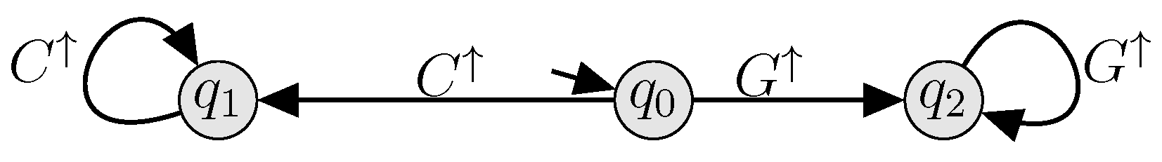
5.1.2. Alternative Dependency
The alternative dependency between the two operations
C and
G, see
Figure 3, may be modeled by four forbidden state combinations as:
. When one of the operations starts to execute, the other must remain initial.
An alternative between a set of operations , is then modeled by an alternative dependency between each pair in the set . In total pairs are required.
5.1.3. Arbitrary Order Dependency
The arbitrary order dependency between the two operation sets
and
, see the leftmost SOP in
Figure 4, may be modeled by seven forbidden state combinations as:
. The combinations require that both
A and
B have to be initial or completed when
C is executing, and the opposite, that
C has to be initial or completed when
A and
B are not both initial or completed. Note that, the combinations add no dependency between
A and
B.
Arbitrary order dependencies between multiple operation sets, as in the SOP for
in
Figure 4, is modeled by an arbitrary order dependency between each pair of the operation sets.
5.1.4. Forced to Complete
In the generic operation automaton, Definition 3, both the initial and the completed states are marked. The supervisor is non-blocking, thus by removing the marking from the initial state, the operation is forced to eventually reach its completed state in the synthesized supervisor.
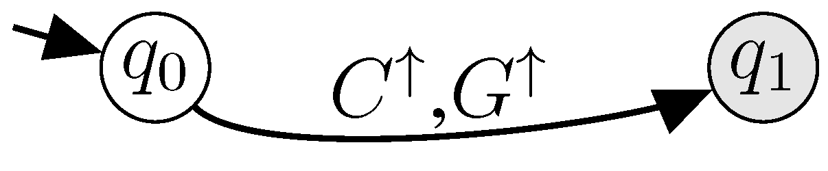
To force one of the operations in an alternative to complete, this removing of marking does not work. Instead the forcing can be modeled through a specification automaton.
Figure 7 illustrates such an automaton for the case when one of the operations
C or
G, in Example 1, is forced to complete. The effect of the automaton is that no states comprising both
and
will be marked, thus one of the operations must complete.
Figure 7.
Specification for forcing one of the operations C or G to complete.
Figure 7.
Specification for forcing one of the operations C or G to complete.
5.2. Nominal Model for Example 1
The four SOPs in
Figure 3 and
Figure 4 constitute the dependencies for the system in Example 1.
Table 1 shows how the dependencies are modeled by forbidden state combinations. Rows 1–7, 8, and 9–12 model precedence, alternative, and arbitrary order dependencies, respectively.
To capture that the operations
are forced to complete, the marking is removed from the initial state in the corresponding five automata. As indicated, to capture that one of the operations
C or
G are forced to complete, the specification automaton in
Figure 7 is added to
.
Table 1.
Forbidden state combinations to model the dependencies for Example 1.
Table 1.
Forbidden state combinations to model the dependencies for Example 1.
| 1 | |
| 2 | |
| 3 | |
| 4 | |
| 5 | |
| 6 | |
| 7 | |
| 8 | |
| 9 | |
| | |
| 10 | |
| | |
| 11 | |
| 12 | |
5.3. The Placement Model
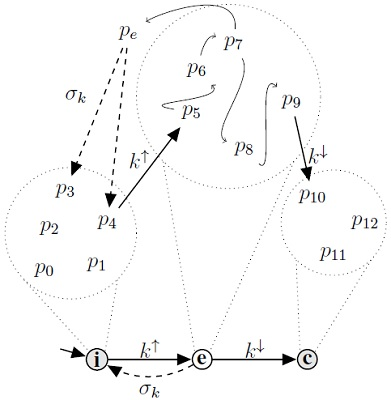
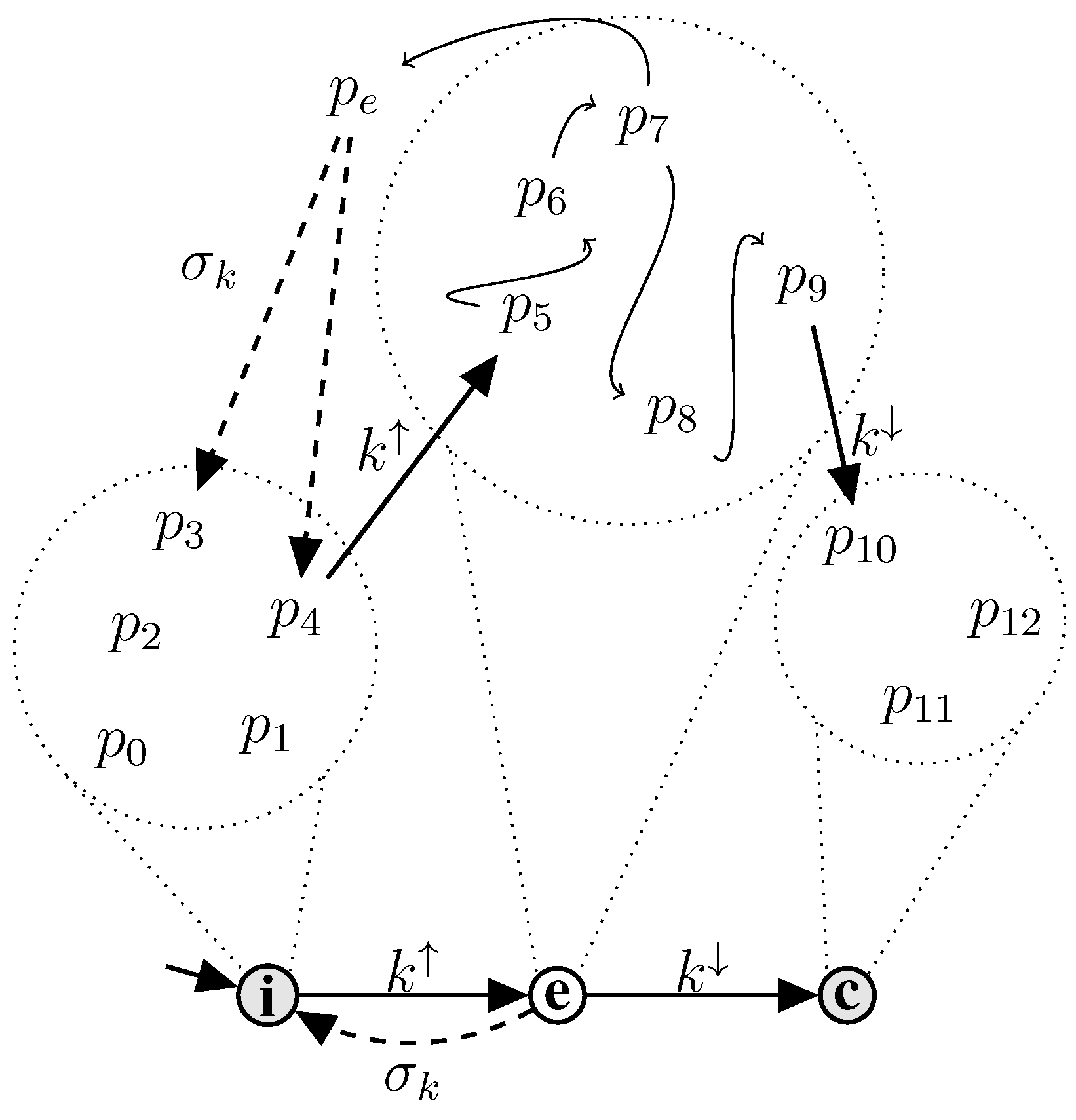
The placement model is the nominal model extended with additional transitions, so called placement transitions. The construction of these placement transitions builds on the definition of upstream states, Definition 6. The intention with each placement transition is to reset to their initial states a potential error operation plus a subset of non-initial operations in the potential error state. The active state of the control system is thereby updated to an upstream state with respect to this potential error operation.
To calculate all restart states that are valid with respect to the dependencies and the reexecution requirements, the placement model must contain the placement transitions such that all potential error operations in all potential error states are connected with all possible upstream states. With such a model, synthesis can be performed to derive the valid restart states as the target states to the placement transitions that are enabled by the supervisor.
The set of possible upstream states for each (potential error) operation is correlated to the set of non-initial operations that can be reset to initial together with k. Let this set be denoted . For each pair , a unique controllable event, a so called placement event, denoted is created.
The reset to initial for
k and the operations in
is then accomplished by adding placement transitions labeled by
to the corresponding operation automata. As pointed out in
Section 4, it is assumed that the potential error operation is in its executing state when an error occurs. Thus, the reset to initial of
k is therefore modeled by a transition
that is added to the transition function
.
In order for the operations in to be upstream after the reset to initial, they have to be non-initial in the potential error state. The reset of each operation is therefore modeled by two transitions and that are added to the transition function .
In the global automaton seen by a synthesis algorithm these locally added placement transitions will synchronize, due to the FSC, and result in a set of placement transitions. All transitions in this set will have the same target state, the upstream state that is to be evaluated as restart state for the potential error operation k.
In the following, let and denote the automata and extended with placement transitions. The set of placement events defined for an operation k is denoted , where , and the set of all defined placement events is denoted , where , such that . If all placement events are constructed, . Given Ω, the placement transitions can be constructed automatically and added to the operation automata.
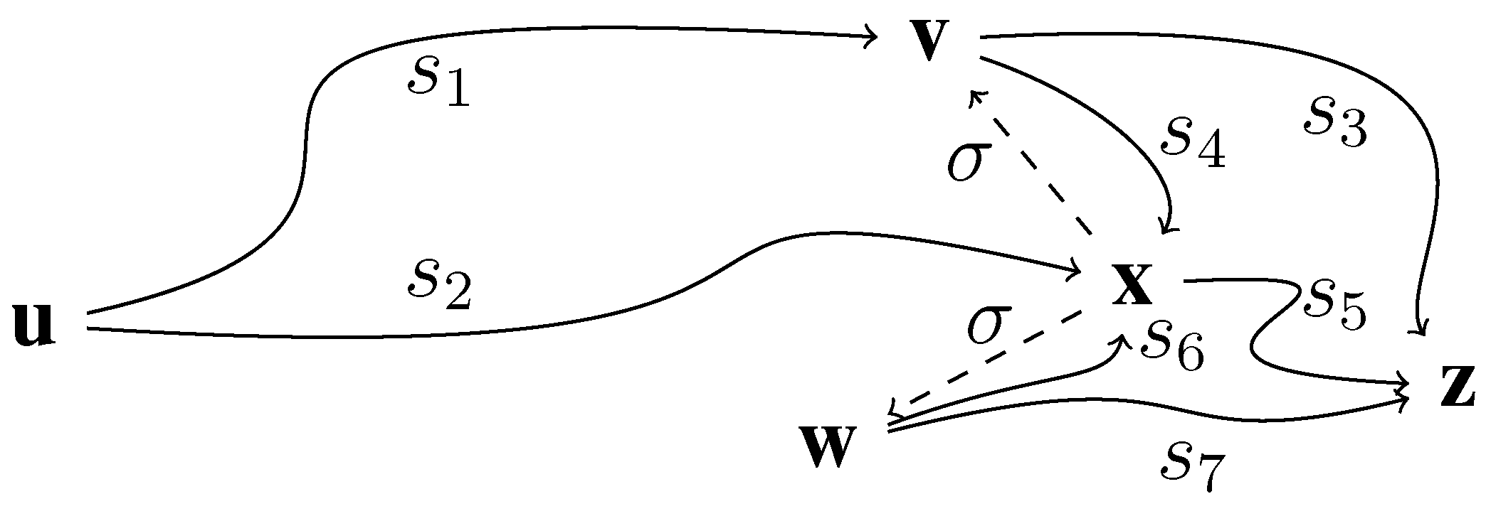
Finally, the modeling of placement transitions is illustrated with the operations B and D from Example 1. There is no dependency between B and D. Let . For clarity, only the placement transitions for D are considered.
Since
, the placement events for
D are
. Where
models reset of just
D and
models reset of both
D and
B. Note the simplification in the indexes, if
is the empty set then it is removed and if it is non-empty then is written as a sequence of the elements. The automaton
is shown in
Figure 8. The state indexes are left out.
Figure 8.
Parallel execution of operations B and D. Placement transitions for D are dashed.
Figure 8.
Parallel execution of operations B and D. Placement transitions for D are dashed.
Operation
D executes in the three states in the middle row of the automaton in
Figure 8. Reset of just
D is allowed in all three executing states, the transitions labeled by
. Reset of both
D and
B is only allowed when
B has started. Thus, the transitions labeled by
can be fired from the two rightmost executing states for
D.
5.4. Synthesis of Restart States
Given the nominal model extended with placement transitions, the restart states that are valid with respect to the dependencies are calculated through synthesis of a supervisor. Synthesis may be seen as a sieve that filters out the restart states that break at least one dependency.
Let the supervisor be denoted
, such that
. It is possible that the dependencies modeled by
are too strict so that no supervisor exists [
26]. In the following discussion, it is therefore assumed that
exists.
An operation
is coupled to its restart states by placement transitions, where each transition is labeled by a placement event
. Guard extraction [
28] is used to find the transitions that are enabled by the supervisor. The target states of the placement transitions that are labeled by
always and
sometimes enabled events are the restart states that are valid with respect to the dependencies.
A transition that is labeled by an always enabled placement event can always be fired when the active state of the automaton coincides with the source state for the transition. A transition that is labeled by a sometimes enabled placement event can, on the other hand, only be fired when the active state of coincides with the source state for the transition and the guard for the event is satisfied in this state.
The modified synthesis algorithm presented in [
5] does not preserve the state dependent behavior for the placement events. Instead, all sometimes enabled placement events are always disabled. The method presented in this paper appends the state dependency to the placement event through the extracted guard, and thereby retains the flexibility to restart even in these cases.
5.5. Restart States for Example 1 Only Based on Dependencies
Let
and
then
and
, thus the introduction of placement transitions introduces more states in the system. Inspection of
shows that one of the two new states is used as a restart state. The state has 12 incoming placement transitions. Note that, this type of restart state is denoted by a
w in
Figure 5. Moreover,
contains 90 always and sometimes enabled placement events.
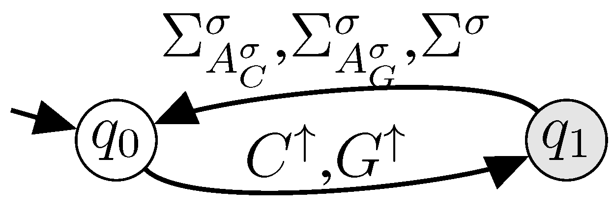
Since the specification automaton in
Figure 7 contains operation events, it has to be extended with placement transitions, as shown in
Figure 9, to enable that the concerned operations can be restarted. In
Figure 9,
and
denote the placement events defined for
C and
G, respectively.
denotes all placement events where
C or
G are among the operations to be reset, that is
.
Figure 9.
Specification in
Figure 7 extended with placement transitions.
Figure 9.
Specification in
Figure 7 extended with placement transitions.
6. To Filter out Simplifying Restart States
Synthesis of the nominal model extended with placement transitions will result in all restart states that are valid in the control system. Despite the fact that a control system state is a valid restart state, it can be hard, and thereby time consuming, for an operator to place the manufacturing in a corresponding physical state. Therefore, this section presents two offline approaches for how to filter out restart states, from this set of valid restart states, where the process to place the manufacturing in a corresponding physical state requires less effort from the operator.
In the first approach, the number of resources to be moved during the restart phase is kept at a minimum. In the second approach, all resources that are affected by the restart are placed in physical state corresponding to home-states.
6.1. To Only Affect Resources of the Error Operation
To simplify for an operator online, the method in [
5] aims to calculate the restart states such that only the resources used to realize the error operations are to be affected in the placement.
It is straightforward to filter out these states. The single requirement is that, all operations that are reset in a placement transition must only be realized by resources also realizing the error operation. For a general placement event , it is then required that .
6.2. Restart from Home-States
A resource is considered to be in a home-state when none of the various operation sequences that it can realize are executing. Due to this non-execution, it is assumed that the resource is idling in the corresponding physical states. It is also assumed that it is rather straightforward for an operator to place the resource in such an idling configuration.
To simplify for an operator, it may therefore be reasonable to filter out the restart states that restart the resources from home-states. Let the control system states corresponding to the home-states for each resource be given as .
Let and denote an error state and its restart state for a general placement transition . Moreover, let denote the set of resources affected by the placement. Thus, these are the resources that are to be moved to home-states during the placement, if they are not already in a home-state.
The state
is a home-state for the resources in
if
. From
Section 5.3, the operation
k and the operations in
are reset to initial with the placement transition, thus
and
. Then, in order to satisfy the home-state condition for the restart state
, knowing that the operations in
are reset to initial, the placement transition should only be fired from the states
where the remaining operations,
, are in operation states such that
is a home-state for the resources in
.
This requirement on the error state may be modeled by an extra home-state condition for when each placement transition can be fired. Given the connection between the operations and the home-states for the resources, it is possible to derive these home-state conditions automatically.
6.3. Home-States in Example 1
In Example 1, it is assumed that a resource is in a home-state if none of the branches in the corresponding arbitrary order SOP is active, see
Figure 4. Thus, as an example, the home-states for resource
correspond to the control system states
.
Given this definition of a home-state, the home-state condition for the transition labeled by the placement event
is discussed for demonstration. The resources to be restarted from home-states are deduced from
Figure 4, this gives
. The operations
E,
C, and
D will be reset to initial by the placement transition. Thus, conditions have to be added for the remaining operations that affect these two resources, that is the operations
A,
B, and
F. Neither
E,
C, nor
D are included in the leftmost branch of the SOP for
. Thus,
A and
B have to be both initial or both completed. In the SOP for
,
F is included in the same branch as
E and
D, thus
F has to be initial since both
E and
F are reset to initial.
Formally this home-state condition can now be expressed as: To place the resources and in home-states, the placement transitions labeled by can only be fired from the states q such that and .
7. To Add Reexecution Requirements
The reexecution requirements constrain how many times and under what circumstances an operation in Ω may be reexecuted. This section demonstrates some examples of such reexecution requirements and how each requirement can be modeled by a specification automaton in order to be included in the supervisor synthesis. By instantiating each reexecution requirement from a type library, it is possible to generate each specification automatically. Reexecution requirements other than those presented in this section can, of course, also be included, as long as the requirement can be modeled by automata.
As defined in
Section 5, the full synchronous composition of all specification automata modeling reexecution requirements is called the
reexecution model and is denoted
. The reexecution requirements do not drive the system, thus all states are marked in the reexecution model, that is
. In the following,
.
As part of the demonstration, three reexecution requirements are placed on the system in Example 1. A filtered subset of the corresponding always and sometimes enabled placement events are given in
Table 2.
The placement events in
Table 2 are filtered according to the two approaches presented in
Section 6. The placement events that only affect the resources used to realize the error operation,
Section 6.1, are shaded in
![Machines 01 00116 i001]()
. The events that model placement of the resources in home-states,
Section 6.2, have
![Machines 01 00116 i002]()
. The placement events that follow both approaches are shaded in
![Machines 01 00116 i003]()
. Always enabled, sometimes enabled, and disabled placement events are marked by ∀, ∃, and −, respectively. Column
n shows the filtered placement events that are enabled by the supervisor when there are no reexecution requirements on the system in Example 1,
Section 5.5.
7.1. Number of Reexecutions
The upper limit for how many times an operation may execute is often connected to the type of process modeled by the operation. Fixation and transport of a product are examples of operations that may typically be reexecuted. Glue applying processes, on the other hand, can typically not be reexecuted.
Without any reexecution requirement, each operation may execute an arbitrary number of times. A specification for how to constrain operation
B to enable zero reexecutions is shown to the left in
Figure 10.
B is then said to be
non-reexecutable. A specification for how to constrain an operation
K to enable at most two reexecutions is given to the right in
Figure 10.
Table 2.
In
![Machines 01 00116 i004]()
placement in home-states, in
![Machines 01 00116 i005]()
placement that only affect resources in error operation, and in
![Machines 01 00116 i006]()
placement in home-states that only affect resources in error operation.
Figure 10.
Specifications that operation B cannot be reexecuted and that operation K can be reexecuted at most two times.
Figure 10.
Specifications that operation B cannot be reexecuted and that operation K can be reexecuted at most two times.
Column
B in
Table 2 shows the always enabled placement events for the system in Example 1 when operation
B is non-reexecutable. As expected, only events that do not reset operation
B are enabled.
7.2. Constrained Reexecution
Constrained reexecution of an operation is often connected to the processing level of a product. For example, predecessor operations to an assembly operation can usually not be reexecuted if the assembly has started.
The specification in
Figure 11 models a requirement where reexecution of operation
D should be prevented when one of the operations
C or
G has started. If
D is the first operation to execute, then the active state of the automaton is updated from
to
. In
neither
C nor
G has started, thus
D may be reexecuted arbitrarily many times. Once
C or
G starts to execute, the active state of the automaton is updated from
to
.
D may not be reexecuted in
. If
C or
G is the first operation to execute, then the active state of the automaton is updated from
to
. From the reexecution requirement, start of
C or
G prevents
D to be reexecuted. Therefore, only a single (the nominal) start of
D is enabled from
.
Figure 11.
Specification that operation D cannot be reexecuted if operation C or G has started.
Figure 11.
Specification that operation D cannot be reexecuted if operation C or G has started.
Column
D in
Table 2 shows always and sometimes enabled placement events when the specification in
Figure 11 is added to the system in Example 1. Restart of the system according to the placement events that affect the operations
D, and
C and/or
G will reset
D to initial. Once
C or
G has started,
D may not be reexecuted. The completed state is the single marked state in
D, thus in order to be non-blocking, the supervisor has to disable these placement events. Thus, all placement events that affect
D, and
C and/or
G are marked as disabled in column
D in
Table 2.
The placement events that affect
D but not
C or
G are marked as sometimes enabled in Column
D. The extracted guards for these events require that neither
C nor
G has started. Thus, the transitions that are labeled by these events can only be fired when
is the active state of the automaton in
Figure 11.
7.3. Set of Reexecuted Operations
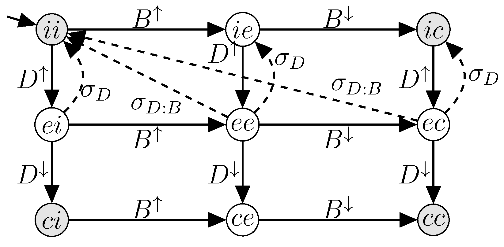
Another type of reexecution requirement is to demand that resetting an operation requires that a set of other operations should also be reset. For example, reseting an operation to fill a vessel could require that an operation to clean the vessel must also be reset.
A requirement that all operations in are to be reset when an operation is reset may be modeled by a specification that disables the placement events that reset without resetting all of the operations in .
Thus, if is reset by a placement transition labeled by an event , that is , then the specification should block this event if , since otherwise the requirement is not satisfied.
Column
in
Table 2 shows always and sometimes enabled placement events when there is a requirement that operation
B has to be reset if operations
C or
G are reset. As expected, Column
is a copy of Column
n where all placement events that affect
C or
G but do not reset
B, are removed.
7.4. Requirements on Branches in Alternatives
The proposed method supports reexecution requirements to constrain which alternative branches that are enabled in the restarted system. A constraint that the first started branch always has to be chosen during restart may be modeled by a specification as in
Figure 12.
Figure 12.
Specification for the alternative operations C and G.
Figure 12.
Specification for the alternative operations C and G.
Let the two operations
C and
G in the alternative in Example 1 be used for demonstration.
Figure 12 shows a specification that models that the first selected branch is always chosen in the restarted system. If
C is the first operation to start then the active state of the automaton is updated from
to
. Only
C is allowed to reexecute in state
. Similarly for
G in state
.
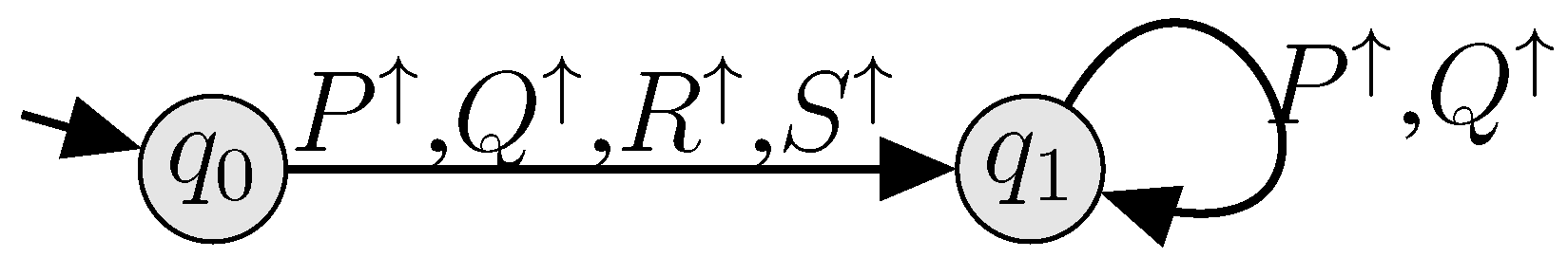
A somewhat similar requirement is to disable a subset of alternative branches in the restarted system. This type of requirement may for example be used to disable automatic inspection in favor of manual inspection in the restarted system.
Figure 13 shows such a specification for an alternative between four operations
, where two,
R and
S, are disabled in the restarted system. The active state of the automaton is updated from
to
when any of the four operations starts. Only
P and
Q may reexecute in state
.
Figure 13.
Specification for disabling operations R and S in a restarted system.
Figure 13.
Specification for disabling operations R and S in a restarted system.


 . The events that model placement of the resources in home-states, Section 6.2, have
  . The placement events that follow both approaches are shaded in
  . Always enabled, sometimes enabled, and disabled placement events are marked by ∀, ∃, and −, respectively. Column n shows the filtered placement events that are enabled by the supervisor when there are no reexecution requirements on the system in Example 1, Section 5.5.
 placement in home-states, in
  placement that only affect resources in error operation, and in
  placement in home-states that only affect resources in error operation.