Control of Adjustable Compliant Actuators

Abstract

Adjustable compliance or variable stiffness actuators comprise an additional element to elastically decouple the actuator from the load and are increasingly applied to human-centered robotic systems. The advantages of such actuators are of paramount importance in rehabilitation robotics, where requirements demand safe interaction between the therapy system and the patient. Compliant actuator systems enable the minimization of large contact forces arising, for example, from muscular spasticity and have the ability to periodically store and release energy in cyclic movements. In order to overcome the loss of bandwidth introduced by the elastic element and to guarantee a higher range in force/torque generation, new actuator designs consider variable or nonlinear stiffness elements, respectively. These components cannot only be adapted to the walking speed or the patient condition, but also entail additional challenges for feedback control. This paper introduces a novel design method for an impedance-based controller that fulfills the control objectives and compares the performance and robustness to a classical cascaded control approach. The new procedure is developed using a non-standard positive-real ${\mathcal{H}}_2$ controller design and is applied to a loop-shaping approach. Robust norm optimal controllers are designed with regard to the passivity of the actuator load-impedance transfer function and the servo control problem. Classical cascaded and positive-real ${\mathcal{H}}_2$ controller designs are validated and compared in simulations and in a test bench using a passive elastic element of varying stiffness.

1. Introduction

Patients with functional deficits due to neurological or orthopedic impairment benefit from robotically-aided motor training, as this leads to an improvement of muscular strength and movement coordination. Manual or machine-assisted treadmill training has existed for more than a decade and is an established therapy for motor impairment occurring, for example, after stroke or spinal cord injury. A multicenter study (DEGAS) in Germany indicates superior results in terms of the activity of daily living (ADL) score of an automated gait trainer (GT 1) compared to conventional physiotherapy training [1]. The repetitions of certain movements during the therapy are assumed to lead to an activation of the central gait pattern generator. The requirements for manipulators in robot-aided therapy differ widely from their counterparts in classical industrial robotics. On the one hand, a patient-cooperative control strategy is needed to allow patient-initiated movement with varying degrees of robotic support. The orthosis or manipulator must be able to allow a variable deviation from pre-defined or continuously calculated joint trajectories, induced by the voluntary movement of the patient. On the other hand, a varying level of spasticity is inherent to patients with functional motor deficits and leads to additional safety requirements for the actuator to avoid large interaction loads in case of a muscle contraction. Furthermore, the patient-load interaction has to be stable for a range of motions with varying degrees of support and resulting stiffness in the patient system. These requirements are contrary to the high stiffness demand in classical robotic applications, which guarantee a high accuracy trajectory tracking. A common requirement in both human-centered and classical robotic applications is a high bandwidth of force/torque and position feedback loops. The idea of impedance control is based on an adjustable torque provided to each joint to control a desired joint trajectory and was introduced in the early 1980s [2]. Following in the early 1990s, compliant actuators were introduced with an elastic decoupling element between the actuator and load [3,4]. The so-called “series elastic actuators” (SEA) were applied to high stiffness hydraulic or electrical actuators and soon found their way into locomotion supportive and assistive technologies. In recent years, compliant actuators were successfully applied to human-centered robotics [5] and with regard to energy storage used in cyclic and explosive movements [6,7]. Successful applications of compliant actuators encompass low torque and position bandwidth applications, such as walking robots [8,9], manipulators for safe human-robot collisions [7,10] and exoskeletons for movement augmentation and rehabilitation use [11,12]. Despite these many successful applications, one of the main drawbacks of compliant actuators can be identified if compared to the biological counterpart, the human or animal musculoskeletal system. The human muscle is connected to the joint with sinews, which provide a nonlinear spring-like behavior. Because of co-antagonistic muscle activation, humans and animals are able to modulate their impedance and cope with a highly uncertain environment. The nonlinear stiffness of the sinews contributes to the mechanical impedance modulation and higher dynamics of the biological musculoskeletal system.

In order to overcome the drawback of limited bandwidth, more advanced compliant actuator approaches consider, for example, nonlinear or adjustable compliant elements. Most recent approaches mimic the biological musculoskeletal system and impedance modulation by the antagonist co-activation of muscles [13,14] or by introducing an additional variable damping term [15,16], leading to additional degrees of freedom in physical impedance transfer function shaping. These new devices, although not limited in bandwidth, are often heavy and require two actuators, one for force/torque generation and one for the adjustment of the stiffness of the compliant element. These disadvantages are not strongly limiting in the case of stationary robots, for example, treadmill training. In such a case, the energy supply and supportive weight can be transferred to the stationary device. A further advantage of compliant actuator technologies is the relatively easily realizable low load impedance with no need for fast sampling high gain control, the damping of high frequency actuator-load oscillations and the relatively cheap force/torque sensor.

In the rehabilitation robotics scenario, two basic strategies of movement support can be differentiated from the structural or kinematic point of view. On the one hand, an end-effector or manipulator-type assistive device is connected to the patient at a single segment or joint. On the other hand, an orthotic exoskeleton type device is connected to single or multiple joints in order to provide assistive torque. In both strategies, the assistive system is connected to the patient, thereby representing mechanically interconnected systems. As a result, the stability and performance of manipulator control cannot be accounted for in an isolated way. Based on a literature review, control strategies for the control of compliant actuators frequently consider PID-type controllers [17]. Even though the stability of the cascaded structures is regarded in most available approaches [18], stability with respect to system uncertainty according to unmodeled dynamics and the stability of the interaction of the manipulator and the patient are most often not considered. An example where the stability of the manipulator-load interaction is explicitly considered in the control design is given by [19]. In this approach, linear PID-type controllers are designed to maintain a positive-real load impedance function. Subsequently, by using the passivity theorem, the interconnection of two passive systems (inherently assuming the load dynamics to be passive) results in a stable system. The drawbacks of this approach are the fixed structure of the controller and the complicated design procedure, with a number of mutually contradictory design requirements. In [20], a SISOloop-shaping approach is presented, which is based on an optimization procedure. The controller parameters are obtained by shaping the load impedance transfer function for a given (fixed) controller structure, where no guarantee for convexity is given for the proposed solution. A convex control design approach is desirable, which inherently guarantees robust stability in the actuator control-loops and for the mechanically interconnected systems by imposing a constraint in terms of a positive-real load impedance function on the controller.

In this contribution, the design and comparison of two different controllers are presented. A norm optimal controller is designed using dissipative ${\mathcal{H}}_2$-synthesis for a modified impedance-based control strategy with the assumption of an adjustable or nonlinear compliant actuator. The synthesized optimal controller is compared to a classical cascaded control structure of the PID-type, designed with regard to a passive actuator load interaction. The positive-real controller does not take into account uncertainty and guarantees interaction stability by the positive realness of the controller and an additional constraint in the design itself. In order to find strictly positive-real (SPR) controllers, norm optimal approaches using the ${\mathcal{H}}_2$ or ${\mathcal{H}}_{\infty }$ framework exist in literature. Lozano-Leal and Joshi [21] and Haddad and Bernstein [22] proposed a procedure for the design of strictly positive-real linear quadratic Gaussian (LQG) controllers and its existence conditions. For a given positive-real plant, the LQG controller obtained from the described procedure is strictly positive-real. These results were extended by Geromel and Gapski [23] in a convex optimization problem. The presented procedure consists of two main steps solving a standard continuous time algebraic matrix Riccati equation (CARE) and a system of linear matrix inequalities (LMI) with an additional constraint that guarantees the positive realness of the controller. This result is used as a basis for a new SPR controller design presented in this contribution. The design problem is rearranged by using a loop-shifting procedure [24], and the LMI problem is reformulated, leading to a feasible problem. The advantage of this new approach is twofold: The use of a norm optimal convex controller procedure minimizing the load impedance function guarantees the best achievable performance in terms of the ${\mathcal{H}}_2$-norm, yet guarantees stability for varying passive load by a strictly positive-real port transfer function. Furthermore, the procedure is not only limited to interaction variable stiffness, but also can be easily extended by variable damping [15,16].

This paper is organized as follows. Section 2 describes the properties of the actuator system, presents a detailed model and introduces a reduced order model. The design of the controllers is given in Section 3. Section 4 describes the experimental test bench and the results. Finally, Section 5 ends with a discussion and conclusion.

2. The Adjustable Compliant Actuator

In this section, the basic principles for compliant actuators are discussed, including a detailed system model with regard to positive-real properties and a reduced order model.

2.1. Compliant Actuators

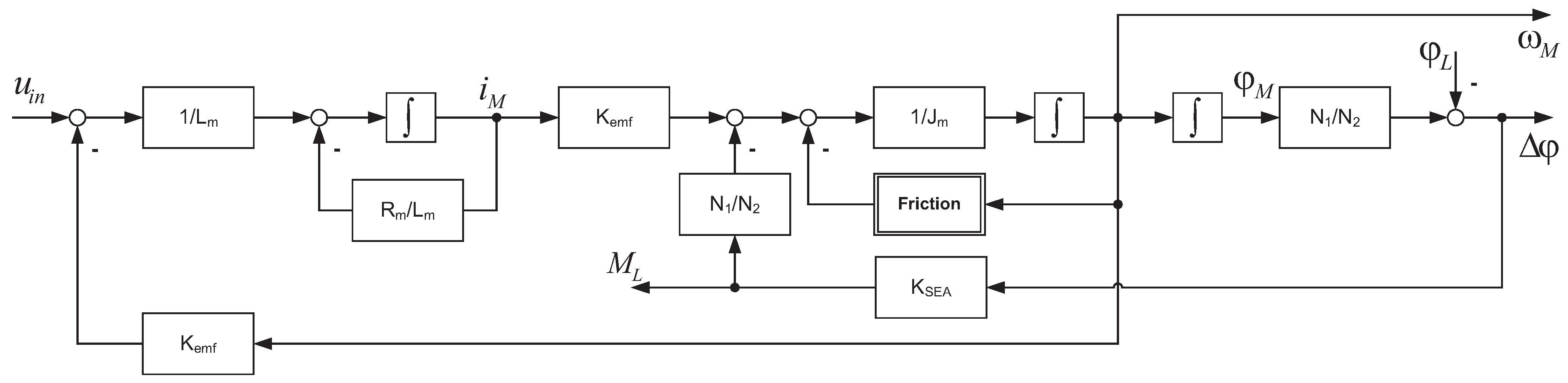
The basic principle of compliant or series elastic actuators (SEA) is to decouple the load from a stiff actuator by introducing a compliant element. Before special compliant actuators were designed, the elasticity between actuator and load was seen as a parasitical element that had to be minimized. In some actuators, like pneumatic or cable-driven designs, the compliant element is inherently given. With this, large loads at manipulator impacts are reduced, even with high impedance controllers. In Figure 1, the basic function of a compliant actuator for an otherwise stiff system is given in a simplified diagram. Assuming the adjustable compliant element between actuator and load to be linear and fixed for frequency analysis, two approximations for the effective inertia at the joint are given for low and high frequency ranges. The decoupling of the inertia takes full effect, especially at high frequencies, which is important to reduce interaction torques. At low frequencies, the reflected motor inertia can be seen, yet the load impedance is greatly reduced by the compliant element, $k_{SEA}$. Besides these inertia decoupling effects, a compliant actuator provides inherent safety, energy storage, a cheap torque sensor system and a reduction of friction effects. However, the main drawbacks are the limited bandwidth, which is associated with the stiffness, $k_{SEA}$, and the need for an extra mechanical element. New designs consider therefore adjustable or nonlinear compliant elements in order to alleviate bandwidth limitations. The advantages of a compliant actuator are highly suitable for supportive or assistive technologies, for manipulators and exoskeletons used in rehabilitation robotics. Bandwidth limitations are not critical, since joint revolutionary speed is relatively slow and further assistance can be given “as needed” with the actuator contributing towards this goal.

Figure 1. The principle of a compliant actuator with the typical setting of the gearbox reduction (top); (a) the high frequency approximation of the effective inertia at the joint $J_{eff}=J_{joint}+N^2{J}_M$; and (b) the low frequency approximation of the effective inertia at the joint $J_{eff}=J_{joint}$.

Figure 1. The principle of a compliant actuator with the typical setting of the gearbox reduction (top); (a) the high frequency approximation of the effective inertia at the joint $J_{eff}=J_{joint}+N^2{J}_M$; and (b) the low frequency approximation of the effective inertia at the joint $J_{eff}=J_{joint}$.

2.2. System Model

The compliant actuator system consists of a brushless direct-current (BLDC) motor with a reduction gearbox. Figure 2 shows the block diagram of the modeled system. The differential equations, Figure 2, describing the system, are given by:

$$\begin{array}{cc}\hfill \frac{d}{dt}{i}_M& =-\frac{R_M}{L_M}{i}_M-\frac{K_{emf}}{L_M}{\omega }_M+\frac{1}{L_M}{u}_{in}\hfill \\ \hfill \frac{d}{dt}{\omega }_M& =\frac{K_{emf}}{J_M}{i}_M-\frac{M_f}{J_M}{\omega }_M-\frac{N_1}{N_2}\frac{K_{SEA}}{J_M}(\Delta \phi ,u_{SEA})\hfill \\ \hfill \frac{d}{dt}{\phi }_M& ={\omega }_M\hfill \end{array}$$

(1)

where ${\phi }_M$, ${\omega }_M$ are the motor angle and speed, $R_M$ and $L_M$ are the electrical motor resistance and inductance and $J_L$ and $K_{emf}$ are the motor inertia and the back-electromagnetic field constant, respectively. Furthermore, $N_1/N_2$ is the gear reduction ratio, $M_f$ is the linearized friction and $K_{SEA}(\Delta \phi ,u_{SEA})$ is the nonlinear adjustable compliant actuator element and is assumed to be a function of $\Delta \phi =\frac{N_1}{N_2}{\phi }_M-{\phi }_L$, with the load angle ${\phi }_L$ and a control input signal, $u_{SEA}$, to change the SEA stiffness. The nonlinear adjustable compliant element is assumed to be sufficiently smooth and linearized for controller design, resulting in a range of SEA values $K_{SEA,\Pi }=[K_{SEA,min},K_{SEA,max}]$, belonging to the family of uncertain parameters, Π. Thus, the output variables of the system are motor rotational speed ${\omega }_M$ and SEA output moment $M_L$, which are given by the linearized output equations:

$$\left[\begin{array}{c}{\omega }_M\\ M_L\end{array}\right]=\left[\begin{array}{ccc}0& 1& 0\\ 0& 0& \frac{N_1}{N_2}{K}_{SEA,\Pi }\end{array}\right]\left[\begin{array}{c}{i}_M\\ {\omega }_M\\ {\phi }_M\end{array}\right]+\left[\begin{array}{cc}0& 0\\ 0& -K_{SEA,\Pi }\end{array}\right]\left[\begin{array}{c}{u}_{in}\\ {\phi }_L\end{array}\right]$$

(2)

The input vector consists of the motor input voltage, $u_{in}$, and the load/joint angle, ${\phi }_L$. The state-space model, obtained by rearranging Equation (1) and Equation (2):

$$\begin{array}{cc}\hfill \frac{d}{dt}\mathbf{x}& ={\mathbf{A}}_{act}\mathbf{x}+{\mathbf{B}}_{act}\mathbf{u}\hfill \\ \hfill \mathbf{y}& ={\mathbf{C}}_{act}\mathbf{x}+{\mathbf{D}}_{act}\mathbf{u}\hfill \end{array}$$

(3)

where $\mathbf{x}\in {\mathbb{R}}^3$, $\mathbf{u}\in {\mathbb{R}}^2$ and $\mathbf{y}\in {\mathbb{R}}^2$, is rearranged with integral action at the input, ${\phi }_L$, to obtain the impedance transfer function $Z\left(s\right)=\frac{M_L\left(s\right)}{{\omega }_L\left(s\right)}$. The resulting matrices using Equation (1) and Equation (2) for the augmented state-space model are:

$$\begin{array}{cc}\hfill {\mathbf{A}}_{act1}& =\left[\begin{array}{cccc}-\frac{R_M}{L_M}& -\frac{K_{emf}}{L_M}& 0& 0\\ \frac{K_{emf}}{J_M}& -\frac{M_f}{J_M}& -{\left(\frac{N_1}{N_2}\right)}^2\frac{K_{SEA}}{J_M}& \frac{N_1}{N_2}\frac{K_{SEA}}{J_M}\\ 0& 1& 0& 0\\ 0& 0& 0& 0\end{array}\right]\hfill \\ \hfill {\mathbf{B}}_{act1}& ={\left[\begin{array}{cccc}\frac{1}{L_M}& 0& 0& 0\\ 0& 0& 0& 1\end{array}\right]}^T\hfill \\ \hfill {\mathbf{C}}_{act1}& =\left[\begin{array}{cccc}0& 1& 0& 0\\ 0& 0& K_{SEA}\frac{N_1}{N_2}& -K_{SEA}\end{array}\right]\hfill \\ \hfill {\mathbf{D}}_{act1}& =\mathbf{0}\hfill \end{array}$$

(4)

with the new input vector $\mathbf{u}={\left[u_{in}{\omega }_L\right]}^T$, the augmented state-vector $\mathbf{x}={\left[i_M{\omega }_M{\phi }_M{\phi }_L\right]}^T$ and the output vector $\mathbf{y}={\left[w_m{M}_L\right]}^T$.

Figure 2. Nonlinear system model of the compliant actuator with the brushless direct-current (BLDC) motor, gearbox reduction and load coupling. Input: $\mathbf{u}={\left[u_{in}{\phi }_L\right]}^T$; and output: $\mathbf{y}={\left[{\omega }_M{M}_L\right]}^T$.

Figure 2. Nonlinear system model of the compliant actuator with the brushless direct-current (BLDC) motor, gearbox reduction and load coupling. Input: $\mathbf{u}={\left[u_{in}{\phi }_L\right]}^T$; and output: $\mathbf{y}={\left[{\omega }_M{M}_L\right]}^T$.

2.3. Current Control and Model Reduction

In order to provide comparable controller results, the current control-loop was closed using a proportional controller in the first step. The current controlled system is then used for SPR-${\mathcal{H}}_2$-synthesis. The gain of the current controller was calculated with the linear quadratic regulator (LQR) approach, thereby minimizing the cost function:

$$J\left(u\right)={\int }_0^{\infty }\left({\mathbf{x}}^T\mathbf{Qx}+u_{in}R{u}_{in}\right)dt$$

(5)

with state weighting matrix $\mathbf{Q}={\mathbf{Q}}^T$ and scalar R for control input weighting. $\mathbf{Q}=\mathrm{diag}(q_1,q_2,0,0)$ is used. The current controller gain, $K_{LQR,i_M}$, resulting from the solution of Equation (5), is incorporated into Equation (4), leading to the state-space model with a new entry at ${\overline{\mathbf{A}}}_{act1}(1,1)=-\frac{1}{L_M}(R_M+K_{LQR,i_M})$, and new control input $\mathbf{u}={\left[u_{in,1}{\phi }_L\right]}^T$. The current controlled system $({\overline{\mathbf{A}}}_{act1},{\mathbf{B}}_{act1},{\mathbf{C}}_{act1},{\mathbf{D}}_{act1})$ is reduced, neglecting high frequency dynamics associated with the current control-loop. Therefore, the augmented state-space model Equation (4) was represented as a transfer function matrix:

$$\mathbf{G}\left(s\right)=\frac{1}{(s+{\alpha }_1)(s^2+{\alpha }_{2}s+{\alpha }_3)}\left[\begin{array}{cc}{\beta }_{11}s& {\beta }_{12}(s+{\alpha }_1)\\ {\beta }_{21}& {\beta }_{22}(s+{\alpha }_1)(s+\gamma )\end{array}\right]$$

(6)

where ${\alpha }_1$, ${\alpha }_2$, ${\alpha }_3$, ${\beta }_{11}$, ${\beta }_{12}$, ${\beta }_{21}$ and ${\beta }_{22}$ are the denominator and numerator coefficients resulting from the state-space model transfer function matrix conversion $\mathbf{G}\left(s\right)={\mathbf{C}}_{act1}{(s\mathbf{I}-{\overline{\mathbf{A}}}_{act1})}^{-1}{\mathbf{B}}_{act1}$. The system Equation (6) has a high-frequency pole corresponding to the electrical system, located at $p_1=-{\alpha }_1=-5.075\times {10}^3$ rad/s. This pole was removed from the model with a subsequent correction of the gains, ${\beta }_{11}$ and ${\beta }_{21}$. As a result, the reduced-order system is compared to the full-order system Equation (6) in Figure 3. The Bode diagram shows a good match up to high frequencies, which are required for torque and impedance control. The high frequency dynamics are nevertheless modeled in a lumped unstructured multiplicative bound for robust control design.

For the design of a strictly positive-real controller, it is important to analyze the positive-realness of the plant. Consider the following lemma:

Lemma 1. (Positive real lemma) Consider the transfer function matrix given by the minimal state-space realization $(\mathit{A},\mathit{B},\mathit{C},\mathit{D})$, $\mathit{G}\left(s\right)=\mathit{C}{\left(s\mathit{I}-\mathit{A}\right)}^{-1}\mathit{B}+\mathit{D}$ to be square. Then, the following statements are equivalent:

• $\mathit{G}\left(s\right)$ is positive-real (PR)
• $\mathit{A}$ is Hurwitz and $\mathit{G}\left(j\omega \right)+\mathit{G}{\left(j\omega \right)}^{*}>0$, $\forall \omega [0,\infty )$ (with ${(·)}^{*}$ denoting the complex conjugate transpose)
• $\exists \mathit{P}={\mathit{P}}^T>0$, such that

  $$\begin{array}{cc}\hfill \mathit{PA}+{\mathit{A}}^T\mathit{P}& =-{\mathit{L}}^T\mathit{L}\hfill \\ \hfill \mathit{PB}& ={\mathit{C}}^T-{\mathit{L}}^T\mathit{W}\hfill \\ \hfill {\mathit{W}}^T\mathit{W}& =\mathit{D}+{\mathit{D}}^T\hfill \end{array}$$

  (7)

It can be easily seen from the phase of the Bode diagram that the reduced order system, as well as the full order system Equation (6) is not positive-real. To analyze the positive realness of the corresponding systems, Statement (2) can be verified via the Nyquist plot or Equation (7) can be rearranged to yield the equivalent LMI-system, where a matrix $\mathbf{P}={\mathbf{P}}^T>0$ is to be found satisfying:

$$\left[\begin{array}{cc}\mathbf{PA}+{\mathbf{A}}^T\mathbf{P}& \mathbf{PB}-{\mathbf{C}}^T\\ {\mathbf{B}}^T\mathbf{P}-\mathbf{C}& -(\mathbf{D}+{\mathbf{D}}^T)\end{array}\right]<0$$

(8)

In the next section, an extended impedance control approach will be presented that leads to a positive-real system for the control.

Figure 3. Bode diagram of the full order (dashed) and the reduced order system. Input: $\mathbf{u}={\left[u_{in,1}{\omega }_L\right]}^T$, output: $\mathbf{y}={\left[{\omega }_M{M}_L\right]}^T$.

Figure 3. Bode diagram of the full order (dashed) and the reduced order system. Input: $\mathbf{u}={\left[u_{in,1}{\omega }_L\right]}^T$, output: $\mathbf{y}={\left[{\omega }_M{M}_L\right]}^T$.

3. Controller Design

Two different approaches, namely a cascaded controller of the PID type and a ${\mathcal{H}}_2$ positive-real controller, are presented in this section for an impedance-based control system design of the compliant actuator. Parameters for classical and robust controllers are given in the Appendix, provided in

Table A2. Controller weightings and parameters for the classical design.

Parameter	Value	Unit	Parameter	Value	Unit
$q_1$	[0.1 0.3 ... 0.7]	-	$q_2$	[5.0 10.0 ... 60.0]	-
R	2.0	-	$K_{LQR}$	[1.43 22.79 1.0]	-
$k_p$	4.0	-	${\tau }_z$	0.2	-
${\tau }_p$	0.028	-	$T_i$	4.0	-
$K_{SEA}$	[50 ... 300]	Nm/rad	$M_f$	[2.0 ... 10]	$\frac{Nms}{rad}$

and

Table A3. Controller weightings and parameters for the robust design.

Parameter	Value	Unit	Parameter	Value	Unit
b	1	-	a	$\frac{4}{5}2\pi$	-
$z_t$	$2\pi$	rad/s	$k_2$	0.1	-
$h_2$	10.0	-	$c_2$	5.0	rad/s
$c_{11}$	1.5	rad/s	$k_{11}$	1,000.0	-
$h_{11}$	0.01	-	$z_{12,HF}$	0.001	s
$z_{12}$	0.0955	s	$p_{12}$	0.0111	s

, respectively.

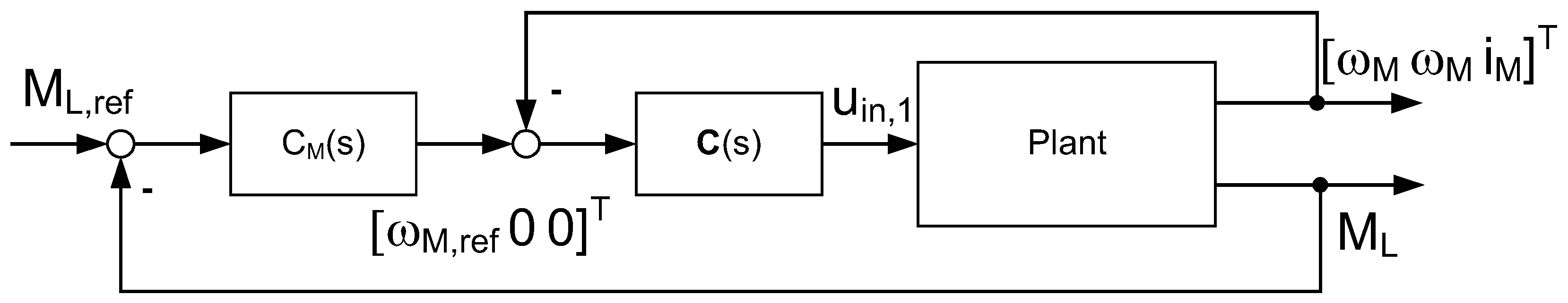
3.1. Cascaded Control Design

A cascaded controller design using PID-type controllers for inner- and outer-loops is presented here. The controller structure is given in Figure 4 and can be divided in an inner, middle and outer loop. The inner-loop consists of the motor current. The middle control-loop is rotary speed feedback, and the outer control-loop is the load torque. For the inner and middle control-loop, a P controller for the current feedback and a PI controller for the motor speed feedback are designed simultaneously, using the LQR-output approach. In the first step, the nonlinear state-space model Equation (3) is linearized with respect to friction and $K_{SEA}$ values, resulting in linear models with outputs ${\mathbf{y}}_c^T=\left[{\omega }_M{\phi }_M\right]$ (refer to the parameters in

Table A1. Parameters used for all simulations.

Parameter	Value	Unit	Parameter	Value	Unit
$R_M$	0.0343	Ω	$L_M$	$0.264\times {10}^{-3}$	H
$K_{emf}$	0.0707	V/rad/s	$I_{max}$	10.0	A
$J_M$	$3.06\times {10}^{-4}$	Nms${}^2$	$M_f$	$7.5\times {10}^{-4}$	$\frac{Nms}{rad}$
$N_1/N_2$	1/160	-	$K_{SEA,nom}$	200.0	$\frac{Nms}{rad}$
${\alpha }_1$	$5.075\times {10}^3$	-	${\alpha }_2$	12.522	-
${\alpha }_3$	12.7908	-	${\beta }_{11}$	$872.697\times {10}^3$	-
${\beta }_{12}$	$2.042\times {10}^3$	-	${\beta }_{21}$	$545.435\times {10}^3$	-
${\beta }_{22}$	−100	-	γ	12.522	-
${\overline{\beta }}_{11}$	171.9	-	${\overline{\beta }}_{21}$	107.48	-
$M_{f0}$	$7.5\times {10}^4$	Nm	$M_{f1}$	$2.0\times {10}^5$	$\frac{Nms}{rad}$

in the Appendix). The feedback controller gains, ${\mathbf{K}}_{lqr}^T\in {\mathbb{R}}^3$, that minimize the quadratic cost function:

$$J\left(u\right)={\int }_0^{\infty }\left({\mathbf{y}}_c^T{\mathbf{Qy}}_c+u_{in}R{u}_{in}\right)dt$$

(9)

are to be determined, where the weighting matrix is defined for the outputs $\mathbf{Q}={\mathbf{Q}}^T\ge 0,\in {\mathbb{R}}^{2\times 2}$, and the control input weighting is $R\in {\mathbb{R}}_{+}$. The minimization of the quadratic cost function Equation (9) is equivalent to the standard-LQR problem with weighting matrices:

$$\left[\begin{array}{cc}\overline{\mathbf{Q}}& \overline{\mathbf{N}}\\ {\overline{\mathbf{N}}}^T& \overline{\mathbf{R}}\end{array}\right]=\left[\begin{array}{cc}{\mathbf{C}}^T& \mathbf{0}\\ {\mathbf{D}}^T& \mathbf{I}\end{array}\right]\left[\begin{array}{cc}\mathbf{Q}& \mathbf{0}\\ \mathbf{0}& \mathbf{R}\end{array}\right]\left[\begin{array}{cc}\mathbf{C}& \mathbf{D}\\ \mathbf{0}& \mathbf{I}\end{array}\right]$$

(10)

For the design of the motor speed control-loop, the parameters of the diagonal matrix, $\mathbf{Q}$ (for example, $Q_{11}=\left[Q_{11,1}\dots Q_{11,n}\right]$), and the scalar, R, are varied over a range of parameters and ${\mathbf{K}}_{lqr,n}$ (refer to Table A2, the Appendix). For the nominal model (Table A1), multiple controllers are designed using each particular weighting matrix value. In a second loop-procedure, the gain and the phase margin of the open-loop compensated plant and the crossover frequency are evaluated over uncertain models (Table A2) and all controllers, ${\mathbf{K}}_{lqr,n}$. The procedure therefore leads to a guaranteed stability margin, since the worst case margins are evaluated over the family of plants containing the parameter uncertainties arising from a variable or nonlinear stiffness, $K_{SEA}$, and motor friction $M_f$. The controller follows from the LQR-output-feedback gain and is augmented with integral action:

$$\mathbf{C}\left(s\right)=\left[\begin{array}{ccc}\frac{K_{lqr,2}}{s}& K_{lqr,1}& K_{lqr,3}\end{array}\right]$$

(11)

where $K_{lqr,3}$ corresponds to the current feedback. Let us now introduce the new output matrix, ${\overline{\mathbf{C}}}_{act1}$, for the augmented state-space model Equation (4), realized by the transfer function:

where ${\overline{\mathbf{C}}}_{act1}$ is defined as:

$${\overline{\mathbf{C}}}_{act1}=\left[\begin{array}{cccc}0& 1& 0& 0\\ 0& 1& 0& 0\\ 1& 0& 0& 0\end{array}\right]$$

and ${\overline{\mathbf{D}}}_{act1}=\mathbf{0}$ of the corresponding dimension. The transfer function for the compensated control-loop is given by:

$${\mathbf{G}}_{OL}\left(s\right)=\overline{\mathbf{G}}\left(s\right)\left[\begin{array}{ccc}& \mathbf{C}\left(s\right)& \\ 0& 0& 1\end{array}\right]$$

(12)

where ${\omega }_M$ is used for proportional and integral feedback and $i_M$ is used for proportional feedback. As a result of the procedure, 480 controller parameter sets were calculated for the family of plants and the variation in parameters of the weighting matrices. The evaluation of inner loop (IL) gain (GM) and phase margin (PM), as well as crossover frequency, leads to a worst case of $G{M}_{IL}=11.7$ dB and $PM=72.6^{\circ }$. The resulting load impedance transfer function for the closed-loop system is positive-real. The controller parameters of the current and speed controller were fixed, since the variation in control performance is small and negligible.

Figure 4. Block diagram of the classical cascaded controller structure (the inner current control-loop is not shown and assumed to be closed).

Figure 4. Block diagram of the classical cascaded controller structure (the inner current control-loop is not shown and assumed to be closed).

For the design of the torque control-loop, the inner-loops, are closed and the torque $M_L$ measured over the elastic element, $K_{SEA}$, is used for feedback. With the closed speed control-loop ${\mathbf{G}}_{\omega ,CL}\left(s\right)$, with inputs ${\mathbf{u}}_{\omega ,CL}^T\left(s\right)=\left[{\omega }_{ref}{\omega }_L\right]$ and outputs ${\mathbf{y}}_{\omega ,CL}^T\left(s\right)=\left[{\omega }_M{M}_L\right]$ follows the compensated motor speed control-loop as:

$${\mathbf{G}}_{OL,M}\left(s\right)={\mathbf{G}}_{\omega ,CL}\left(s\right)\left[\begin{array}{cc}{C}_M\left(s\right)& 0\\ 0& 1\end{array}\right]$$

(13)

with the torque controller, $C_M\left(s\right)$. The torque controller is designed as a PI controller with additional lead-phase correction (“lead-lag”) at the crossover frequency:

$$C_M\left(s\right)=k_p\left(\frac{T_{i}s+1}{s}\right)\frac{{\tau }_{z}s+1}{{\tau }_{p}s+1}$$

(14)

A nominal value of $K_{SEA}=200$ Nm/rad was used for the controller design. As an initial controller parameter setting, the controller dynamics were adjusted according to the disturbance dynamics $G_d\left(s\right)=\frac{M_L}{{\omega }_L}$. In a second step, the gain margin of the controller is determined by continuous adaption of $k_p$ for the critical case of a fixed load. Finally, the parameter, $T_i$, is used to determine the controller bandwidth up to a minimal phase margin of $PM={40}^{\circ }$. The lead-lag compensator is designed to increase the phase margin to at least $PM={60}^{\circ }$. As a result of the procedure and varying stiffness $K_{SEA}$, the worst case gain and phase margins were determined to be $GM=24.15$ dB and $PM=65.{16}^{\circ }$. The controller procedure leads to a positive-real load impedance transfer function, although the positive realness of the load impedance transfer function was not explicitly addressed in the controller design (to obtain, for example, controller parameter bounds as a result of the additional constraint [19]).

3.2. Augmented Torque Control

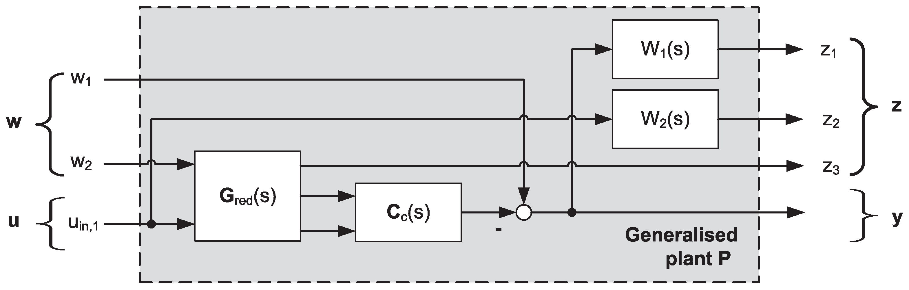
In this section, the concept of augmented torque control is presented, which is the basis for the SPR-${\mathcal{H}}_2$ controller design. Based on the parameters given in Table A3 (Appendix), the plant considered here is the current controlled plant Equation (4) with outputs ${\mathbf{y}}^T=\left[{\omega }_M{M}_L\right]$ and the reduced input vector $u_{in,1}$. A post-compensator is applied to down-square the system, leading to a phase lead at the crossover frequency. Consider the non-square transfer function of the reduced order system Equation (6),

$${\mathbf{G}}_{red}\left(s\right)=\frac{1}{s^2+{\alpha }_{2}s+{\alpha }_2}\left[\begin{array}{c}{\overline{\beta }}_{11}s\\ {\overline{\beta }}_{21}\end{array}\right]$$

(15)

for which the post-compensator is to be synthesized. The next steps of the down-squaring procedure use the Smith–McMillan form to determine transmission zeros and poles. Based on Equation (15), the Smith and the Smith–McMillan matrices are given by:

$$\begin{array}{cc}\hfill \mathbf{S}\left(s\right)& =\left[\begin{array}{c}1\\ 0\end{array}\right]\hfill \\ \hfill \mathbf{M}\left(s\right)& =\left[\begin{array}{c}\frac{1}{s^2+{\alpha }_{2}s+{\alpha }_2}\\ 0\end{array}\right]\hfill \end{array}$$

(16)

where the Smith-form is obtained using the decomposition and the following unitary polynomial matrices, $\mathbf{U}\left(s\right)$ and $\mathbf{V}\left(s\right)$:

$$\mathbf{U}\left(s\right)\mathbf{S}\left(s\right)\mathbf{V}\left(s\right)=\left[\begin{array}{cc}\frac{{\overline{\beta }}_{11}}{{\overline{\beta }}_{21}}s& 1\\ 1& 0\end{array}\right]\left[\begin{array}{c}1\\ 0\end{array}\right]{\overline{\beta }}_{21}=\left[\begin{array}{c}{\overline{\beta }}_{11}s\\ {\overline{\beta }}_{21}\end{array}\right]$$

(17)

Given a fixed structure post-compensator $\mathbf{C}\left(s\right)=\left[ab\right]$, the set of transmission zeros is obtained by solving:

$$\text{det}\left({\mathbf{C}}_c\left(s\right)·\left[\begin{array}{c}\frac{{\overline{\beta }}_{11}}{{\overline{\beta }}_{21}}s\\ 1\end{array}\right]\right)$$

and the resulting position of the transmission zero of the open-loop compensated transfer function:

$$z_t=-\frac{{\overline{\beta }}_{21}}{{\overline{\beta }}_{11}}·\frac{b}{a}$$

The zero position is determined by fixing the gain $b=1$, such that the load torque is entirely accounted for in the feedback. The gain corresponding to the motor speed is chosen to guarantee a phase increase of about 90${}^{\circ }$ at the crossover frequency ${\omega }_{CR}\left(K_{SEA}\right)=[12.6\dots 25.1]$ rad/s, while maintaining the same steady-state gain as compared to the torque transfer function $u_{in,1}\left(s\right)\to M_L\left(s\right)$. Therefore, for low frequencies, the torque control feedback-loop characteristic is maintained in the augmented torque control structure. The compensated plant used for further controller design is denoted by:

$${\mathbf{G}}_2\left(s\right)={\mathbf{C}}_c\left(s\right){\mathbf{G}}_{red}\left(s\right)$$

(18)

and is extended with an additional output, ${\phi }_L$. The compensated plant is positive-real for all possible values of $K_{SEA}$.

3.3. Strictly Positive-Real ${\mathcal{H}}_2$ Controller Design

A new approach to augmented torque control with load impedance minimization is presented that is based on a convex optimization procedure proposed in [23] and extended to the generalized plant with relaxed orthogonality assumptions here. The output compensated plant Equation (18) is used as a basis for the controller design, which results in a strictly positive-real controller, optimal in the sense that the ${\mathcal{H}}_2$ closed-loop transfer function norm is minimized for a square plant. The key point in the procedure is that the load impedance function is incorporated into the plant, in order to guarantee a positive real load-actuator interaction by the controller. Towards that goal, the plant is extended with complex weightings and is brought to the generalized control configuration, for which an overview is shown in Figure 5. Since plant orthogonality assumptions were presumed in the original approach [23], the procedure is extended with a so-called loop-shifting procedure [24] to relax the original assumptions.

Figure 5. Generalized plant for augmented torque control with additional constraint in terms of the impedance function $Z\left(s\right)=\frac{z_3\left(s\right)}{w_2\left(s\right)}$.

Figure 5. Generalized plant for augmented torque control with additional constraint in terms of the impedance function $Z\left(s\right)=\frac{z_3\left(s\right)}{w_2\left(s\right)}$.

Design weightings are used to specify the control performance of the compensated load torque and load angle, with design weightings of first-order, for example:

$$W_2\left(s\right)=c_2\frac{z_{2}s+1}{p_{2}s+1}$$

(19)

where parameters determined from:

$$z_2=\sqrt{\frac{k_2^2{c}_2^2(1-h_2^2)}{h_2^2(k_2^2-1)}},p_2=\sqrt{\frac{c_2^2(1-h_2^2)}{k_2^2-1}}$$

(20)

and $k_2$ is the static gain, $z_2$ is the zero inverse and $p_2$ is the pole inverse of the transfer function and are calculated according to Equation (20). The gain at low and high frequency is chosen as $k_2=0.1$ and $h_2=10$ to penalize control effort, where the $c_2=5$ rad/s is set-up according to actuator bandwidth and limits the duty-cycle of the actuator. The performance of the mixed torque/motor speed feedback loop is weighted with $W_1\left(s\right)$ applied to the corresponding sensitivity function. $W_1\left(s\right)=W_{11}\left(s\right)W_{12}\left(s\right)$ is specified as a second-order transfer function consisting of a lead-lag part and a low-pass. The lead-lag is specified with a crossover-frequency of $c_{11}=1.5$ rad/s. The gain at low and high frequency is fixed at $k_{11}=1000$ and $h_{11}=0.01$, which corresponds to a steady-state error of 0.001 and a sufficient roll-off at high frequencies for low and high gain, respectively. To keep the augmented plant a positive-real system, the weighting, $W_{11}\left(s\right)$, is extended with a first-order lead-lag filter and a high frequency lag given by:

$$W_{12}\left(s\right)=\frac{z_{12}s+1}{p_{12}s+1}\frac{1}{z_{12,HF}s+1}$$

(21)

which introduces phase advance near the crossover frequency and guarantees the generalized plant matrix ${\mathbf{D}}_{11}=\mathbf{0}$, because of the high-frequency lag, $z_{12,HF}$. The generalized plant can be derived from the interconnection structure in Figure 5 as:

$$\mathbf{P}\left(s\right)=\left[\begin{array}{ccc}{W}_1\left(s\right)& 0& -W_1\left(s\right){\mathbf{C}}_c\left(s\right){\mathbf{G}}_{red,21}\left(s\right)\\ 0& 0& W_2\left(s\right)\\ 0& {\mathbf{G}}_{red,11}\left(s\right)& 0\\ 1& 0& -{\mathbf{C}}_c\left(s\right){\mathbf{G}}_{red,21}\left(s\right)\end{array}\right]$$

(22)

with nominal parameters corresponding to high-stiffness values of the compliant actuator element. The transfer function Equation (22) is rearranged in a minimal realization state-space model given by:

$$\begin{array}{cc}\hfill \frac{d}{dt}\mathbf{x}& =\mathbf{Ax}+{\mathbf{B}}_1\mathbf{w}+{\mathbf{B}}_2\mathbf{u}\hfill \\ \hfill \mathbf{z}& ={\mathbf{C}}_1\mathbf{x}+{\mathbf{D}}_{12}\mathbf{u}\hfill \\ \hfill \mathbf{y}& ={\mathbf{C}}_2\mathbf{x}+{\mathbf{D}}_{21}\mathbf{w}\hfill \end{array}$$

(23)

with the following dimensions: $\mathbf{x}\in {\mathbb{R}}^n$ the state vector, $\mathbf{u}\in {\mathbb{R}}^m$ the control input, $\mathbf{y}\in {\mathbb{R}}^p$ the controller input, $\mathbf{w}\in {\mathbb{R}}^r$ the disturbance and $\mathbf{z}\in {\mathbb{R}}^q$ the control objective. Based on the model structure, the following conditions apply for the plant. The resulting conditions for Equation (23) are:

• ($\mathbf{A},{\mathbf{B}}_1,{\mathbf{C}}_1,$) is controllable and observable
• ($\mathbf{A},{\mathbf{B}}_2,{\mathbf{C}}_2,$) is controllable and observable
• ${\mathbf{D}}_{12}^T{\mathbf{D}}_{12}>0$ and ${\mathbf{D}}_{21}{\mathbf{D}}_{21}^T>0$.

The conditions are satisfied for the plant Equation (23), but a violation of the orthogonality assumptions, as required for the standard ${\mathcal{H}}_2$-problem, can be determined. Note that orthogonality assumptions ${\mathbf{D}}_{12}^T{\mathbf{C}}_1=\mathbf{0}$ and ${\mathbf{D}}_{21}{\mathbf{B}}_1^T=\mathbf{0}$ are required in the SPR-${\mathcal{H}}_2$ approach presented in [23].

Consider the closed-loop transfer function given by the lower linear fractional transformation (LFT) ${\mathbf{H}}_{\mathbf{zw}}\left(s\right)={\mathcal{F}}_l(\mathbf{P}\left(s\right),\mathbf{C}\left(s\right))$, with the disturbance input, $\mathbf{w}$, and disturbance outputs, $\mathbf{z}$. Then, the problem of finding a strictly positive-real controller, $\mathbf{C}\left(s\right)$, can be stated by the minimization problem [23]:

$$\min \left({∥{\mathbf{H}}_{\mathbf{zw}}\left(s\right)∥}_2^2:\mathbf{C}\left(s\right)\in {\mathcal{P}}_C\right)$$

(24)

with ${\mathcal{P}}_C$ denoting the family of strictly positive-real transfer functions. Different solutions exist in the literature, which rely on varying assumptions about the plant. For example, [21,22] assume plant conditions that lead to a standard ${\mathcal{H}}_2$-problem. In contrast to this approach, [25] presents a fixed-order dynamic compensator approach in which an upper bound to the ${\mathcal{H}}_2$-norm is given for ${\mathbf{H}}_{\mathbf{zw}}\left(s\right)$, and optimality conditions are stated in terms of Riccati and Lyapunov equations for the positive-real plant, for which a dual formulation is presented in [26]. Since the procedure requires ${\mathbf{D}}_{12}^T{\mathbf{C}}_1=\mathbf{0}$ and ${\mathbf{D}}_{21}{\mathbf{B}}_1^T=\mathbf{0}$, a modification is proposed in this paper, which is based on a loop-shifting procedure [24] and a reformulation of the LMI-procedure [27]. In order to lift the plant orthogonality constraints, consider the singular value decomposition:

$$\begin{array}{cc}\hfill {\mathbf{D}}_{12}& ={\mathbf{U}}_{12}\left[\begin{array}{c}\mathbf{0}\\ {\Sigma }_{12}\end{array}\right]{\mathbf{V}}_{12}^T\hfill \\ \hfill {\mathbf{D}}_{21}& ={\mathbf{U}}_{21}\left[\begin{array}{cc}\mathbf{0}& {\Sigma }_{21}\end{array}\right]{\mathbf{V}}_{21}^T\hfill \end{array}$$

(25)

which is introduced for the change of generalized plant coordinates:

$$\begin{array}{cc}\mathbf{w}={\mathbf{S}}_{\mathbf{w}}\tilde{\mathbf{w}}:={\mathbf{V}}_{21}^T\tilde{\mathbf{w}}& \mathbf{u}={\mathbf{S}}_{\mathbf{u}}\tilde{\mathbf{u}}:={\Sigma }_{12}^{-1}{\mathbf{V}}_{12}^T\tilde{\mathbf{u}}\\ \mathbf{z}={\mathbf{S}}_{\mathbf{z}}^{-1}\tilde{\mathbf{z}}:={\mathbf{U}}_{12}\tilde{\mathbf{w}}& \mathbf{y}={\mathbf{S}}_{\mathbf{y}}^{-1}\tilde{\mathbf{y}}:={\mathbf{V}}_{21}{\Sigma }_{21}\tilde{\mathbf{y}}\end{array}$$

(26)

Subsequent rearranging of transformations to the block-diagonal matrices: ${\mathcal{N}}_i=\mathrm{diag}\left(\mathbf{I},{\mathbf{S}}_{\mathbf{w}},{\mathbf{S}}_{\mathbf{u}}\right)$ and ${\mathcal{N}}_o=\mathrm{diag}\left(\mathbf{I},{\mathbf{S}}_{\mathbf{z}},{\mathbf{S}}_{\mathbf{y}}\right)$, results in the following plant transformation:

$$\tilde{\mathbf{P}}=\left[\begin{array}{ccc}\mathbf{A}& {\tilde{\mathbf{B}}}_1& {\tilde{\mathbf{B}}}_2\\ {\tilde{\mathbf{C}}}_1& \mathbf{0}& \left[\begin{array}{c}\mathbf{0}\\ \mathbf{I}\end{array}\right]\\ {\tilde{\mathbf{C}}}_2& \left[\begin{array}{cc}\mathbf{0}& \mathbf{I}\end{array}\right]& \mathbf{0}\end{array}\right]={\mathcal{N}}_o\mathbf{P}{\mathcal{N}}_i$$

(27)

The observer continuous-time matrix Riccati equation (CARE) associated with the full ${\mathcal{H}}_2$ control problem:

$$\begin{array}{cc}\hfill {\mathbf{AY}}_2+& {\mathbf{Y}}_2{\mathbf{A}}^T+{\mathbf{B}}_1{\mathbf{B}}_1^T\hfill \\ & -({\mathbf{Y}}_2{\mathbf{C}}_2^T+{\mathbf{B}}_1{\mathbf{D}}_{21}^T){\left({\mathbf{D}}_{21}{\mathbf{D}}_{21}^T\right)}^{-1}({\mathbf{C}}_2{\mathbf{Y}}_2+{\mathbf{D}}_{21}{\mathbf{B}}_1^T)=\mathbf{0}\hfill \end{array}$$

(28)

can be rearranged by using Equation (27) to:

$$\begin{array}{cc}\hfill {\mathbf{Y}}_2(\mathbf{A}& -{\tilde{\mathbf{B}}}_1{\tilde{\mathbf{D}}}_{21}^T{\tilde{\mathbf{C}}}_2{)}^T+(\mathbf{A}-{\tilde{\mathbf{B}}}_1{\tilde{\mathbf{D}}}_{21}^T{\tilde{\mathbf{C}}}_2){\mathbf{Y}}_2\hfill \\ & -{\mathbf{Y}}_2{\tilde{\mathbf{C}}}_2^T{\tilde{\mathbf{C}}}_2{\mathbf{Y}}_2+{\tilde{\mathbf{B}}}_1{\mathbf{E}}_2{\tilde{\mathbf{B}}}_1^T=\mathbf{0}\hfill \end{array}$$

(29)

where ${\mathbf{E}}_2=\mathrm{diag}({\mathbf{I}}_{(r-p)\times (r-p)},{\mathbf{0}}_{p\times p})$. If the associated Hamiltonian matrix:

$${\mathbf{H}}_2=\left[\begin{array}{cc}{(\mathbf{A}-{\tilde{\mathbf{B}}}_1{\tilde{\mathbf{D}}}_{21}^T{\tilde{\mathbf{C}}}_2)}^T& -{\tilde{\mathbf{C}}}_2^T{\tilde{\mathbf{C}}}_2\\ -{\tilde{\mathbf{B}}}_1{\mathbf{E}}_2{\tilde{\mathbf{B}}}_1^T& -(\mathbf{A}-{\tilde{\mathbf{B}}}_1{\tilde{\mathbf{D}}}_{21}^T{\tilde{\mathbf{C}}}_2)\end{array}\right]$$

(30)

has no imaginary axis eigenvalues, ${\mathbf{Y}}_2=\mathrm{ric}\left({\mathbf{H}}_2\right)$ is the stabilizing solution leading to the observer feedback matrix: $\mathbf{L}={\mathbf{L}}_2={\mathbf{Y}}_2{\tilde{\mathbf{C}}}_2^T+{\tilde{\mathbf{B}}}_1{\tilde{\mathbf{D}}}_{21}^T$ of the controller structure:

$$\begin{array}{cc}\hfill \frac{d}{dt}{\mathbf{x}}_c& ={\mathbf{Ax}}_c+{\tilde{\mathbf{B}}}_2\mathbf{u}+{\mathbf{L}}_2(\mathbf{y}-{\tilde{\mathbf{C}}}_2{\mathbf{x}}_c)\hfill \\ \hfill \mathbf{u}& =-\mathbf{K}{\mathbf{x}}_c\hfill \end{array}$$

(31)

with the controller transfer function given by:

$${\tilde{\mathbf{C}}}_K=\mathbf{K}{(s\mathbf{I}-[{\mathbf{A}}_K-{\mathbf{L}}_2{\tilde{\mathbf{C}}}_2])}^{-1}{\mathbf{L}}_2$$

(32)

where ${\mathbf{A}}_K=\mathbf{A}-{\tilde{\mathbf{B}}}_2\mathbf{K}$. Now, given the controller transfer function Equation (32) in the coordinates of Equation (27), the procedure to obtain a strictly positive-real controller is reformulated in this approach. Towards that goal, define the fixed matrices ${\mathbf{A}}_2:=\mathbf{A}-{\mathbf{L}}_2{\tilde{\mathbf{C}}}_2$ and ${\mathbf{Q}}_2:={\tilde{\mathbf{B}}}_2{\mathbf{L}}_2^T+{\mathbf{L}}_2{\tilde{\mathbf{B}}}_2^T$, and linear matrix inequality:

$$\mathbf{W}{\mathbf{A}}_2^T+{\mathbf{A}}_2\mathbf{W}-{\mathbf{Q}}_2\le -ϵ\mathbf{I}<0$$

(33)

the matrix variable $\mathbf{W}={\mathbf{W}}^T>0$, an arbitrary small parameter $ϵ>0$ and controller gain matrix $\mathbf{K}={\mathbf{L}}_2^T{\mathbf{W}}^{-1}+{\tilde{\mathbf{D}}}_{12}^T{\tilde{\mathbf{C}}}_1$. Then, for a symmetric matrix $\mathbf{Z}={\mathbf{Z}}^T\in {\mathbb{S}}^q$, the performance index:

$$J=\min \mathrm{tr}\left(\mathbf{Z}\right)$$

is to be minimized for the system of LMI’s:

$$\begin{array}{cc}\hfill \left[\begin{array}{cc}\mathbf{W}& {({\mathbf{C}}_1\mathbf{W}-{\mathbf{D}}_{12}{\mathbf{L}}_2^T)}^T\\ {\mathbf{C}}_1\mathbf{W}-{\mathbf{D}}_{12}{\mathbf{L}}_2^T& \mathbf{Z}\end{array}\right]& \ge 0\hfill \\ \hfill \mathbf{AW}+{\mathbf{WA}}^T-{\mathbf{Q}}_2+{\mathbf{L}}_2\left({\mathbf{D}}_{21}{\mathbf{D}}_{21}^T\right){\mathbf{L}}_2^T& \le -ϵ\mathbf{I}\hfill \end{array}$$

(34)

If the minimization problem for Equation (33) and Equation (34) has a solution in the variables, $\mathbf{W}$ and $\mathbf{Z}$, a gain matrix $\mathbf{K}={\mathbf{L}}_2^T{\mathbf{W}}^{-1}+{\tilde{\mathbf{D}}}_{12}^T{\tilde{\mathbf{C}}}_1$ can be calculated, such that the resulting controller belongs to the family of strictly positive transfer functions. The proof assuming orthogonal plant conditions was described in [23]. However, with the relaxed orthogonality constraint, the rearranged problem can be applied to a wider range of loop-shaping applications. In addition, the system of rearranged LMI’s Equation (34) is suitable to loop-shaping problems, since the matrix, $\mathbf{Z}\in {\mathbb{R}}^{q\times q}$, has typically higher dimension and leads to a feasible LMI-problem with the proposed example. The controller in the coordinate system of the generalized plant is finally obtained by using the transformation:

$${\mathbf{C}}_K\left(s\right)={\mathbf{S}}_y^{-1}{\tilde{\mathbf{C}}}_K\left(s\right){\mathbf{S}}_u^{-1}$$

(35)

A strictly positive-real controller of the eighth-order was calculated using the convex optimization toolbox, Yalmip [28].

4. Simulation and Experimental Results

Classical and robust controllers are verified in simulation and experimental tests.

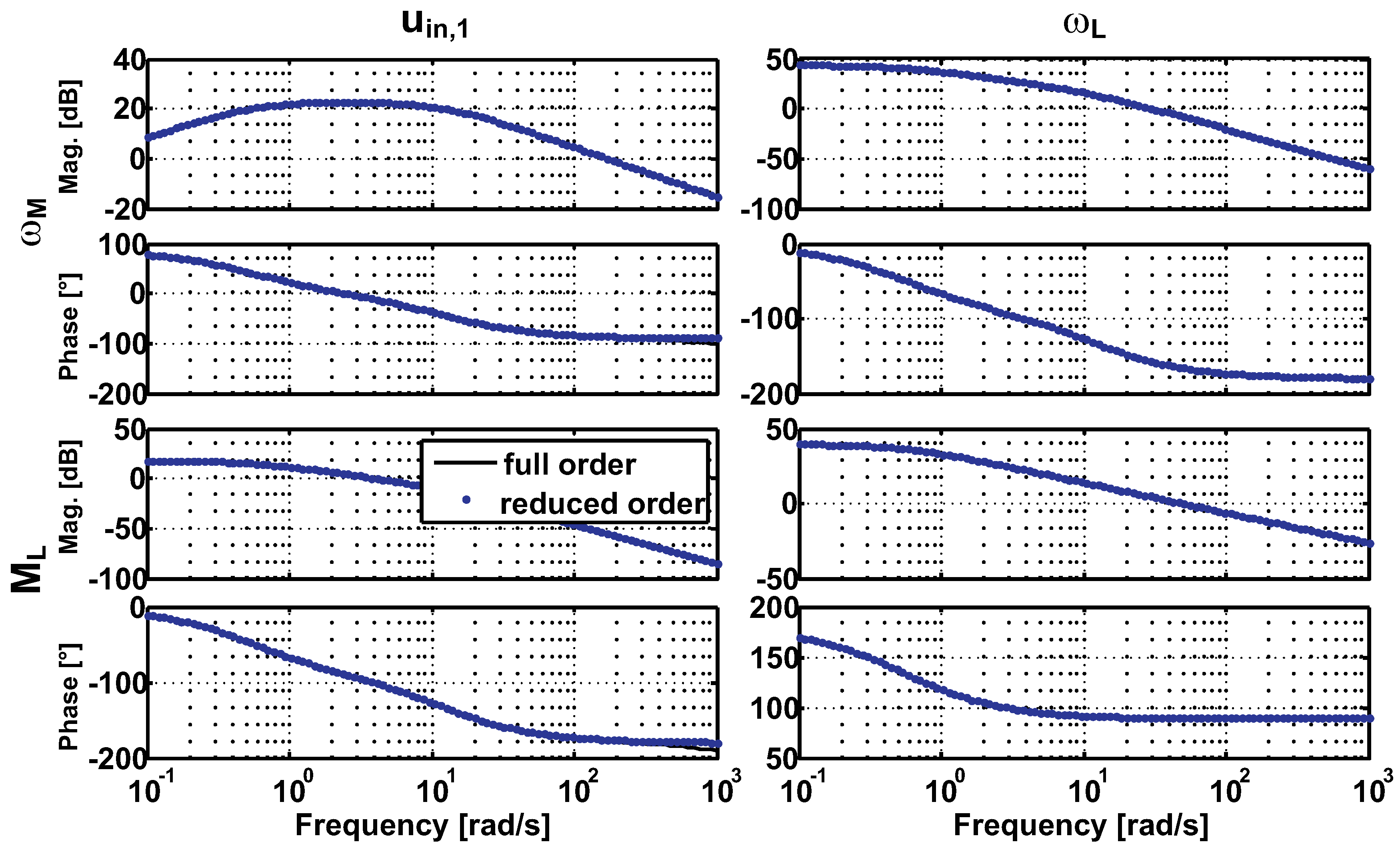
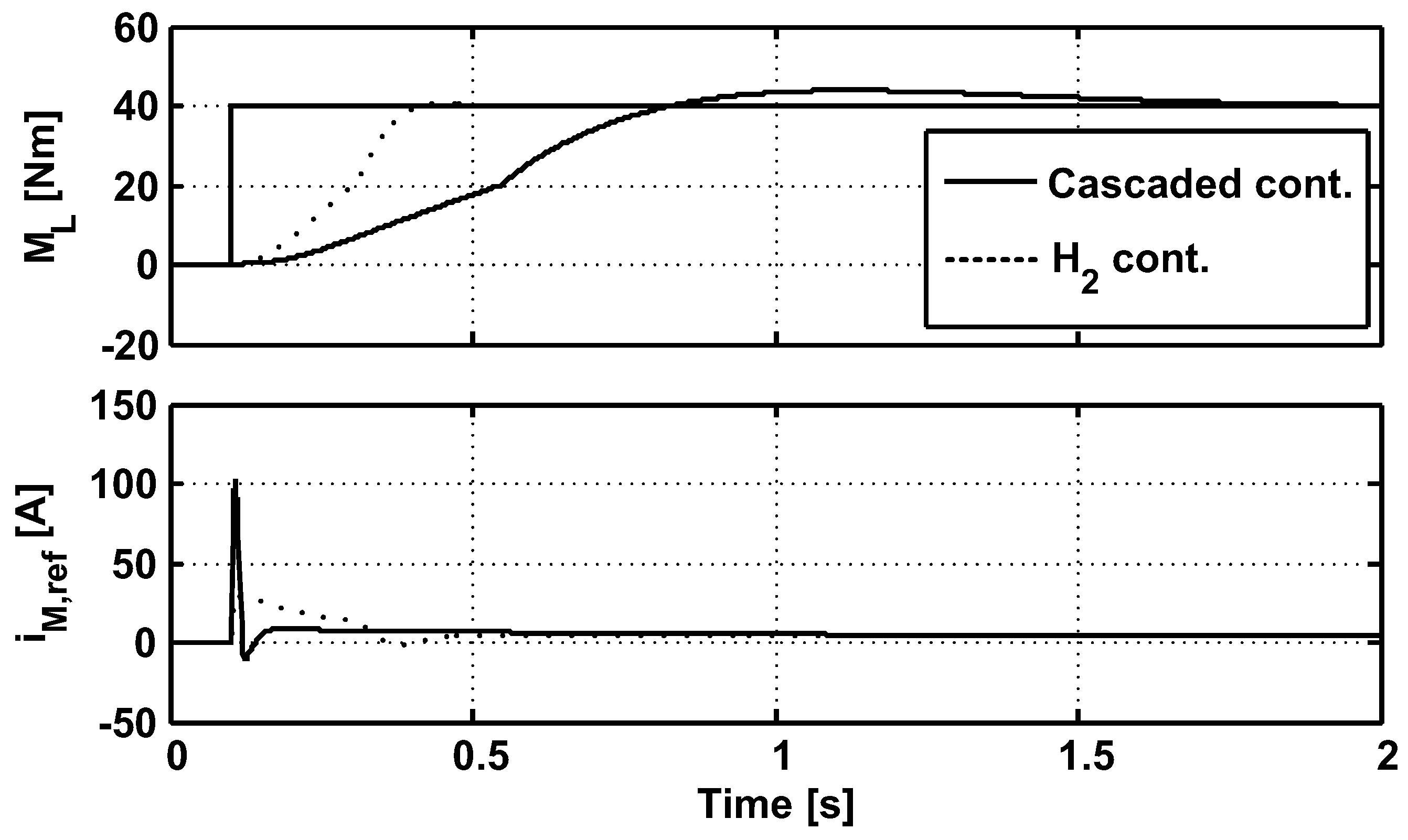
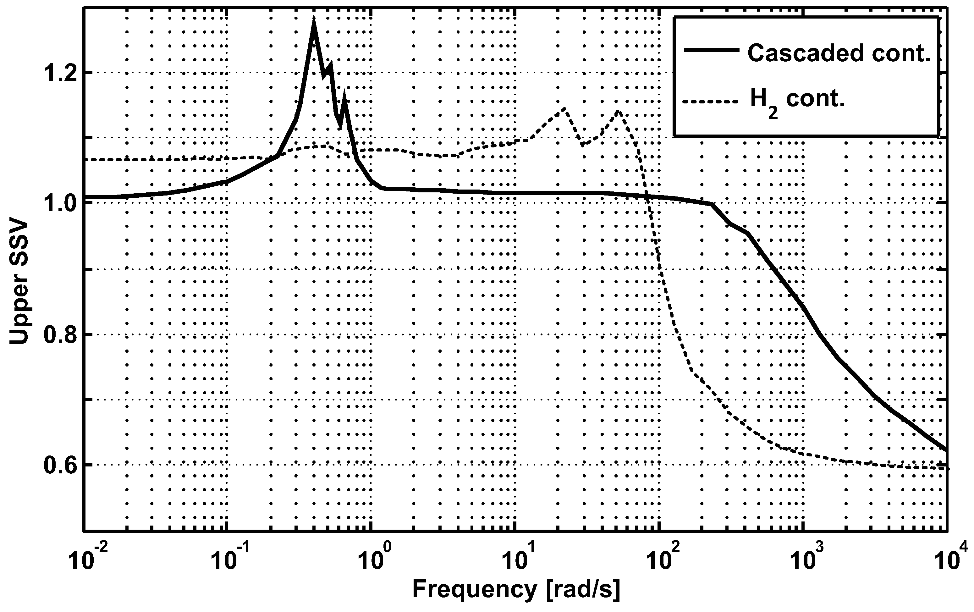
4.1. Simulation Results

The performance and robustness of the designed controllers were first verified in simulations using a detailed nonlinear model of the mechanical setup described in Section 4.2. On the one hand, the compliant actuator element was modeled as a bilinear element consisting of two different stiffness values in order to allow a greater torque range:

$$K_{SEA}(\Delta \phi )=\left\{\begin{array}{ccc}\hfill K_{SEA,1}& \forall \hfill & \hfill 0\le |\Delta \phi |<0.2\mathrm{rad}\\ \hfill K_{SEA,2}& \forall \hfill & \hfill |\Delta \phi |\ge 0.2\mathrm{rad}\end{array}\right.$$

(36)

On the other hand, the $M_f$ was modeled as a nonlinear Coulomb friction:

$$M_f\left({\omega }_M\right)=(\mathrm{sgn}\left({\omega }_M\right)M_{f0}+M_{f1}){\omega }_M$$

(37)

with the system friction lumped into $M_f$ and no additional terms for the test bench modeled, thereby assuming an ideal gearbox. The motor current limitation was included in the model, and classical and robust controllers were extended with additional anti-windup logic consisting of the current value of the motor current reference and a high gain feedback technique. The controller performance was evaluated at fixed load conditions, corresponding to the worst case test in terms of plant dynamics. Furthermore, the controller performance was tested using typical load conditions. Figure 6 shows the step responses of the torque control-loop at fixed load conditions ${\phi }_L=0$. This corresponds to the worst-case gain scenario in the loop, as the envelope of the reference torque crosses through the nonlinear stiffness range.

Figure 6. Torque control step response at fixed load conditions ${\phi }_L=0$ with nonlinear compliant element $K_{SEA}(\Delta \phi )$.

Figure 6. Torque control step response at fixed load conditions ${\phi }_L=0$ with nonlinear compliant element $K_{SEA}(\Delta \phi )$.

At a torque of $M_L=20$ Nm, the effect of the nonlinear stiffness can be seen, where $K_{SEA}$ increases from 100 Nm/rad to 250 Nm/rad. The resulting step response of the cascaded classical controller presents the slowest response with an overshoot slightly below 10% of the reference value. The ${\mathcal{H}}_2$ controller shows a step response with much faster ±10% settling times of about 270 ms compared to 640 ms in case of the classical cascaded controller. Besides controller performance tests, the robust stability of the two different controllers was determined using the linearized system model with real and complex uncertainty. The complex bound was modeled at the input of the plant according to neglected model dynamics and lumped parameter uncertainties. The uncertainty corresponding to neglected dynamics and discretization is modeled as lumped unstructured multiplicative input uncertainty for the corresponding family of plants:

$${\mathbf{G}}_p\left(s\right)=(1+w_m\left(s\right){\Delta }_m\left(s\right))\mathbf{G}\left(s\right)$$

(38)

with $\mathbf{G}\left(s\right)$ denoting the transfer function of the nominal model Equation (18). The upper bound for $w_m\left(s\right)$ was chosen by evaluating uncertain transfer functions, $G_p\left(j\omega \right)$, in the family of plants, Π:

$$l_m\left(\omega \right)=\underset{G_p\left(j\omega \right)\in \Pi }{max}\left(({\mathbf{G}}_p\left(j\omega \right)-\mathbf{G}\left(j\omega \right)){\mathbf{G}}^{-1}\left(j\omega \right)\right),\forall \omega$$

(39)

for which $l_m\left(\omega \right)\le \left|w_m\left(s\right)\right|$. The weighting function was modeled as a first-order lead-lag transfer function Equation (19) and was determined by low frequency gain $k_m=0.05$, high-frequency gain $h_m=1.5$ and crossover frequency $c_m=300$ rad/s. The low and high gains thereby correspond to a total lumped uncertainty of 5% and 50%, respectively. Furthermore, a passive load was modeled consisting of real uncertain parameters, $K_{SEA}$, $M_f$, $m_L$ and $d_L$, where $m_L$ and $d_L$ are the load mass and damping, respectively. The result of the stability analysis is given in Figure 7. The upper bound for the ${\mathcal{H}}_2$ and the classical controller are 1.14 and 1.27, respectively, implying no guarantee for robust stability as a result of the μ-analysis. However, a second robust stability analysis with reduced load dynamics resulted in guaranteed robust stability with a structured singular value smaller than 0.7 for the two controllers. Furthermore, the load impedance transfer functions of the two controllers are positive-real, indicating the stability of the designed torque controllers with respect to any passive dynamic load function. Thus, for the described uncertainty, the μ-analysis is assumed to give conservative results. However, a certain tendency towards guaranteed stability is obtained for the different control approaches, indicating a higher stability bound for the ${\mathcal{H}}_2$ controller at the augmented torque loop crossover frequency and a lower stability margin of the classical controller in the lower frequency range.

Figure 7. Upper structured singular value (SSV) of the classical cascaded and augmented torque ${\mathcal{H}}_2$ controller.

Figure 7. Upper structured singular value (SSV) of the classical cascaded and augmented torque ${\mathcal{H}}_2$ controller.

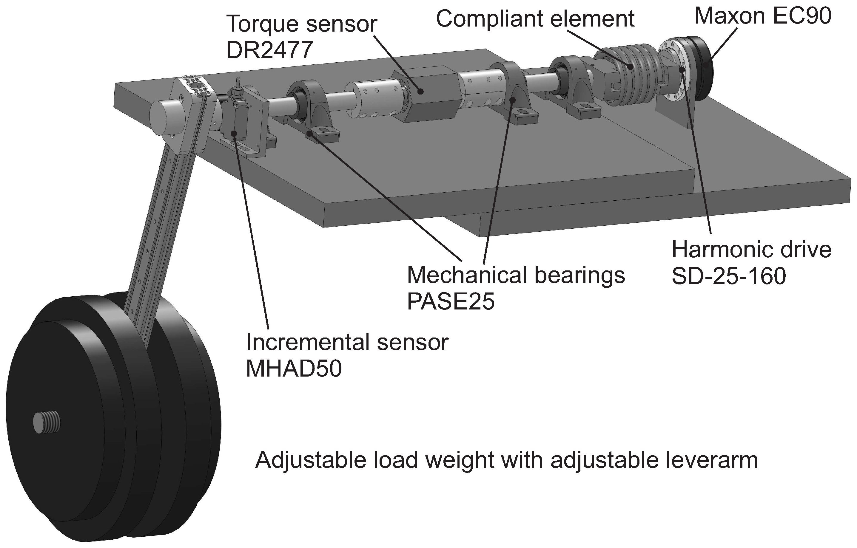
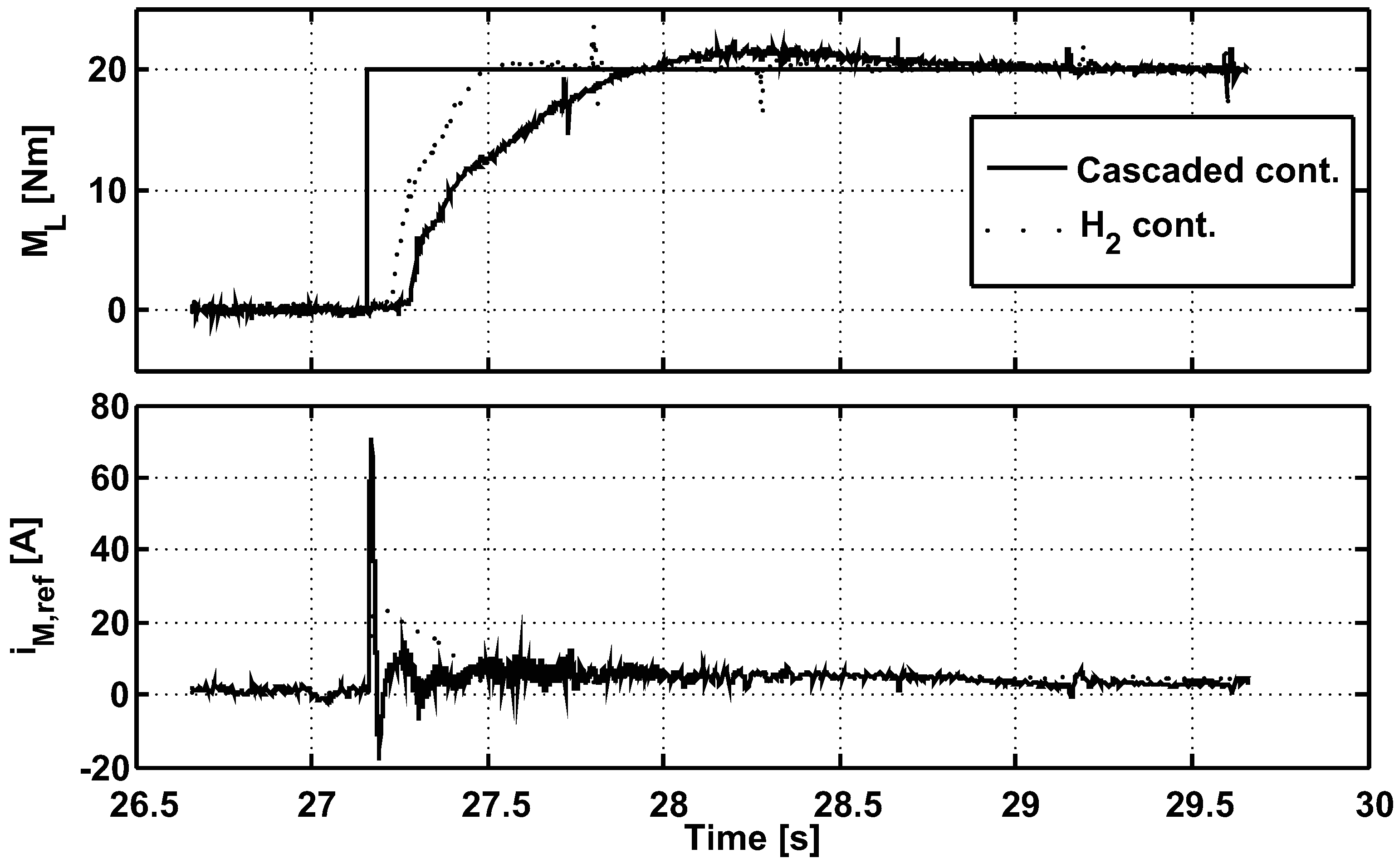
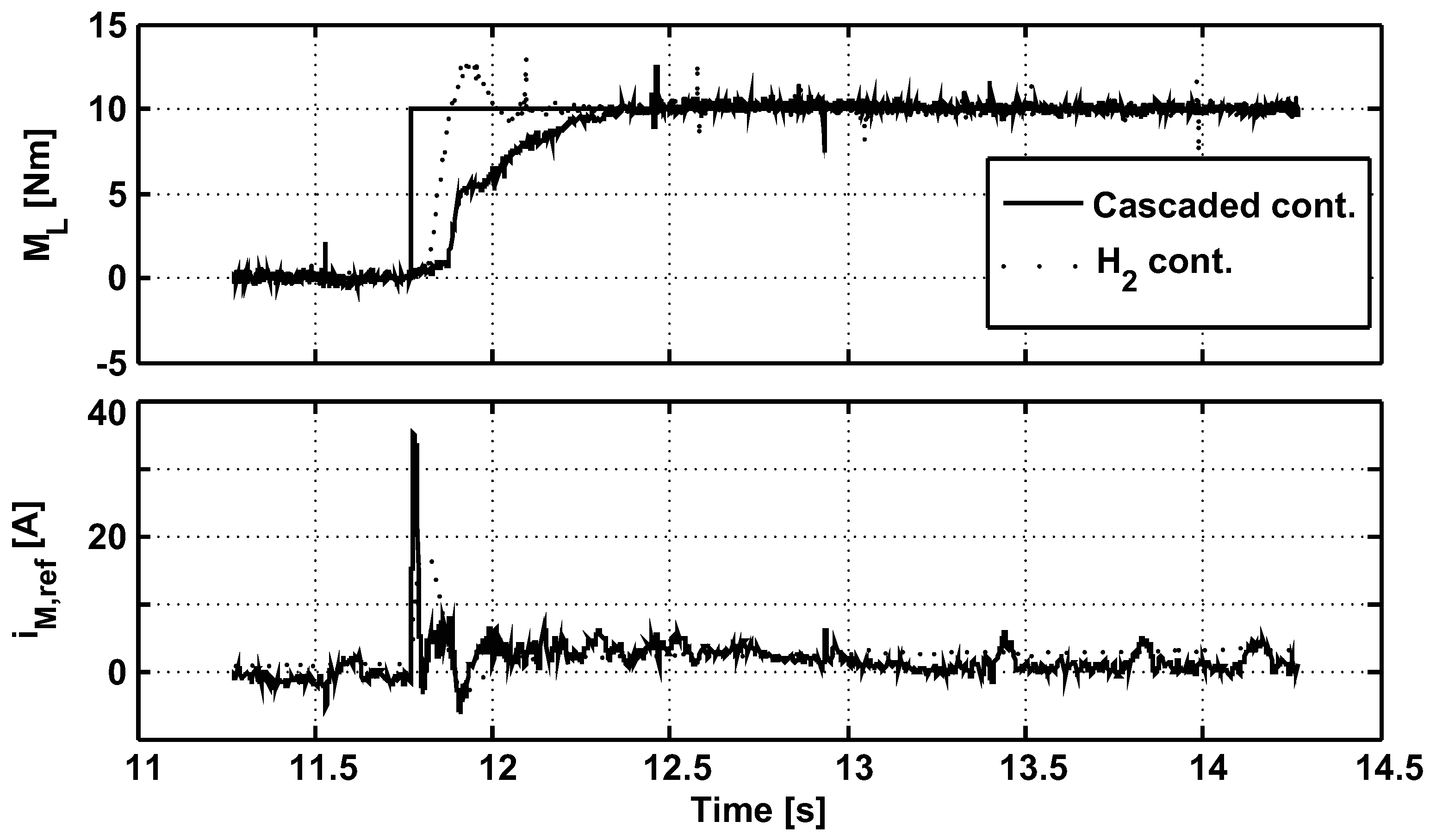
4.2. Experimental Study

The experimental test bench consists of a brushless direct-current motor (EC90 Flat, Maxon, Switzerland), a gear reduction (SD-25-160, Harmonic Drive, Japan), a supported rotating shaft and a variable load (which can be optionally fixed). For the support of the rotating shaft, mechanical bearings (PASE25, INA, Germany) were used. In addition to the motor sensors (Encoder MILE, Maxon, Switzerland), a torque sensor (DR2477, Lorenz Messtechnik, Germany) and an incremental encoder (MHAD50, Baumer, Germany) were applied to measure the load torque and angle, respectively. Figure 8 shows a CAD-drawing of the test bench. The BLDC motor is controlled by a current driver unit (E-DARC-M, Eckelmann AG, Germany), which receives current reference values from a dSPACE unit (dSPACE 1103, dSPACE AG, Germany). The controllers were implemented in MATLAB/Simulink in discretized form with a sampling time of $T_s=2.5$ ms. The communications of the sensors were arranged via the controller area network (CAN) bus, except for the load torque sensor and the motor current reference, which was sampled using the analog input/output card of the dSPACE unit. The controllers, which were designed for a range of stiffness values of the compliant element, were validated in control performance tests using the load torque step responses of different amplitudes. The tests were conducted with different stiffness values of the compliant element, using mechanical springs of varying sizes, instead of a nonlinear or continuously adaptable stiffness element. Figure 9 shows the typical result of an experiment at a stiffness of the compliant element of $K_{SEA}=100$ Nm/rad and an amplitude of the reference step of 20 Nm.

Figure 8. Test bench with exchangeable compliant element and adjustable load (mass and lever arm).

Figure 8. Test bench with exchangeable compliant element and adjustable load (mass and lever arm).

Figure 9. Experimental load torque control step response at fixed load conditions ${\phi }_L=0$ with compliant element $K_{SEA}=100$ Nm/rad.

Figure 9. Experimental load torque control step response at fixed load conditions ${\phi }_L=0$ with compliant element $K_{SEA}=100$ Nm/rad.

The performance of the controllers in the real plant is similar to results obtained from simulation. However, in the experiment, the compliant element is linear, resulting in a slightly larger settling time. Comparing classical and optimal controller performance, it can be seen that, similar to simulation, the settling time is almost doubled with the ${\mathcal{H}}_2$ controller. Figure 10 shows a step response to a reference change of $M_{L,ref}$ from 0 to 10 Nm. The overshoot of the ${\mathcal{H}}_2$ controller it is about 25%, where in the case of the classical controller, no overshoot can be observed. Similar results of controller performance were achieved in a series of step responses of different amplitudes and at different stiffness values of the compliant element. At commanded reference values of a higher amplitude, the controller responses are mostly determined by the motor current saturation limitation, which leads to a reduction of excessive overshoot. A comparison of the controllers is provided in Table 1. The simulation performance measures in the table belong to the step response tests with the bilinear element in Figure 6. The experimental performance measurements correspond to the step response of $M_{L,ref}=10$ Nm at a stiffness of the compliant element of 250 Nm/rad.

Figure 10. Experimental load torque control step response at fixed load conditions ${\phi }_L=0$ with compliant element $K_{SEA}=250$ Nm/rad.

Figure 10. Experimental load torque control step response at fixed load conditions ${\phi }_L=0$ with compliant element $K_{SEA}=250$ Nm/rad.

Table 1. Controller comparison (settling time (ST), overshoot (OS), integral of absolute errors (IAE), integral of square errors (ISAE)).

Criterion	Classical Controller	${\mathcal{H}}_2$-Controller
$\overline{\mu }\left(\mathbf{M}\left(j\omega \right)\right)$	1.27	1.14
$\pm 10\%$ ST (ms) (SIM)	640	270
OS (%) (SIM)	9.7	1.1
IAE (-) (SIM)	9.4	3.7
ISAE (-) (SIM)	249.7	115.1
$\pm 10\%$ ST (ms) (EXP)	440	220
OS (%) (EXP)	-	25
IAE (-) (EXP)	0.887	0.49
ISAE (-) (EXP)	4.81	2.36
$\mathrm{var}(i_{M,ref}-{\overline{i}}_{M,ref})$	0.73	0.024

Table 1. Controller comparison (settling time (ST), overshoot (OS), integral of absolute errors (IAE), integral of square errors (ISAE)).

Criterion	Classical Controller	${\mathcal{H}}_2$-Controller
$\overline{\mu }\left(\mathbf{M}\left(j\omega \right)\right)$	1.27	1.14
$\pm 10\%$ ST (ms) (SIM)	640	270
OS (%) (SIM)	9.7	1.1
IAE (-) (SIM)	9.4	3.7
ISAE (-) (SIM)	249.7	115.1
$\pm 10\%$ ST (ms) (EXP)	440	220
OS (%) (EXP)	-	25
IAE (-) (EXP)	0.887	0.49
ISAE (-) (EXP)	4.81	2.36
$\mathrm{var}(i_{M,ref}-{\overline{i}}_{M,ref})$	0.73	0.024

The comparison of the controllers in simulation and experiments shows that the ${\mathcal{H}}_2$ controller not only provides lowest errors in terms of the integral of absolute errors (IAE) and the integral of square errors, but also has the best settling time and overshoot in simulation. The classical cascaded controller has an overshoot of about 10% in simulation and in experiments at lower stiffness values of the compliant element. However, towards higher stiffness values, the overshoot decreases. Finally, if comparing the variance of the average mean free controller output, $i_{M,ref}-{\overline{i}}_{M,ref}$, where $i_{M,ref}$ is the reference input for the motor current control circuit, much lower values can be observed for the ${\mathcal{H}}_2$-controller. This corresponds to a lower energy consumption, as strongly needed in mobile rehabilitation robotics applications, and is provided by the higher frequency roll-off of the robust ${\mathcal{H}}_2$ controller.

5. Conclusions and Discussion

A new control strategy was developed for torque control with actuator-inherent compliance. By introducing a down-squaring procedure of the plant with an output compensator, the zero of the square transfer function was placed in order to achieve a phase advance and a positive-real transfer function. The torque control thereby bypasses a cascaded controller design, as usually conducted in the classical design, and can be reliably utilized by modern robust control design procedures.

Important advantages of the proposed procedure are the low frequency properties of the down-squared system, which correspond to the load torque measured over the compliant element, thereby conserving the properties of the impedance transfer function for the outer-loop controller. Based on a validated model, a new robust controller was developed for the augmented torque control and compared to a classical cascaded controller of the PID type. The robust controller was designed by assuming the load to be passive, thereby guaranteeing the interaction stability for varying load. Robustness towards a changing compliant element was guaranteed by a following μ-analysis and not explicitly in the design. For the design of the strictly positive-real ${\mathcal{H}}_2$ controller, the actuator-load interaction was constrained by a positive-real transfer function and incorporated into the design procedure. In the case of the ${\mathcal{H}}_2$ controller, a reliable trade-off between robustness and performance properties could be observed in simulations and on a test-bench. The robust controller surpasses the classical controller in terms of settling time and actuator duty cycle. In terms of a low number of tuning parameters and the inherent passivity constraint, the ${\mathcal{H}}_2$ controller seems most promising for the nonlinear/time-varying compliant actuator application. As a simple scheduling procedure, a combined blending/conditioning scheme could be used in terms of the measured load torque output. Further extension of the proposed mixed algebraic matrix Riccati-LMI design procedure to an SPR-${\mathcal{H}}_2$ linear-parameter-varying approach is suggested to increase the performance. This extension and the application of the robust augmented torque control approach to a rehabilitation robotics application are issues of ongoing work.

References

1. Pohl, M.; Werner, C.; Holzgraefe, M.; Kroczek, G.; Wingendorf, I.; Holig, G.; Koch, R.; Hesse, S. Repetitive Locomotor Training and Physiotherapy Improve Walking and Basic Activities of Daily Living After Stroke: A Single-Blind, Randomized Multicentre Trial (DEutsche GAngtrainerStudie, DEGAS). Clin. Rehabil. 2007, 21, 17–27. [Google Scholar] [CrossRef] [PubMed]
2. Hogan, N. Impedance Control: An Approach to Manipulation: Part I-III. J. Dyn. Syst. Meas. Control 1985, 107, 1–24. [Google Scholar] [CrossRef]
3. Pratt, G.; Williamson, M. Series Elastic Actuators. In Proceedings of the IEEE/RSJ International Conference on Intelligent Robots and Systems, Pittsburgh, PA, USA, 5–9 August 1995; pp. 399–406.
4. Pratt, G.A.; Williamson, M.M.; Dillworth, P.; Pratt, J.; Wright, A. Stiffness Isn’t Everything. In Proceedings of the 4th International Symposium (Experimental Robotics IV), Stanford, CA, USA, 30 June–2 July 1995; Springer: Berlin/Heidelberg, Germany, 1997; pp. 253–262. [Google Scholar]
5. Zinn, M.; Khatib, O.; Roth, B.; Salisbury, J. Actuation Methods for Human-Centered Robotics and Associated Control Challenges. In Control Problems in Robotics; Springer: Berlin/Heidelberg, Germany, 2003; Volume 4, pp. 105–119. [Google Scholar]
6. Vanderborght, B.; Verrelst, B.; van Ham, R.; van Damme, M.; Lefeber, D.; Duran, B.M.Y.; Beyl, P. Exploiting Natural Dynamics to Reduce Energy Consumption by Controlling the Compliance of Soft Actuators. Int. J. Robot. Res. 2006, 24, 343–358. [Google Scholar] [CrossRef]
7. Grebenstein, M.; Albu-Schaffer, A.; Bahls, T.; Chalon, M.; Eiberger, O.; Friedl, W.; Gruber, R.; Haddadin, S.; Hagn, U.; Haslinger, R.; et al. The DLR Hand Arm System. In Proceedings of the IEEE International Conference on Robotics and Automation, Shanghai, China, 9–13 May 2011; pp. 3175–3182.
8. Schuitema, E.; Hobbelen, D.; Jonker, P.; Wisse, M.; Karssen, J. Using a Controller Based on Reinforcement Learning for a Passive Dynamic Walking Robot. In Proceedings of the IEEE/RAS International Conference on Humanoid Robots, Tsukuba, Japan, 5–7 December 2005; pp. 232–237.
9. Collins, S.; Ruina, A. A Bipedal Walking Robot with Efficient and Human-Like Gait. In Proceedings of the IEEE International Conference on Robotics and Automation, Barcelona, Spain, 18–22 April 2005; pp. 1983–1988.
10. Diftler, M.; Mehling, J.; Abdallah, M.; Radford, N.; Bridgwater, L.; Sanders, A.M.; Askew, R.S.; Linn, D.; Yamokoski, J.; Permenter, F.; et al. Robonaut 2—The First Humanoid Robot in Space. In Proceedings of the IEEE International Conference on Robotics and Automation, Shanghai, China, 9–13 May 2011; pp. 2178–2183.
11. Veneman, J.; Ekkelenkamp, R.; Kruidhof, R.; van der Helm, F.; van der Kooij, H. A Series Elastic- and Bowden-Cable-Based Actuation System for Use as Torque Actuator in Exoskeleton-Type Robots. Int. J. Robot. Res. 2006, 25, 261–281. [Google Scholar] [CrossRef]
12. Karavas, N.; Tsagarakis, N.; Caldwell, D. Design, Modeling and Control of a Series Elastic Actuator for an Assistive Knee Exoskeleton. In Proceedings of the 4th IEEE/RAS/EMBS International Conference on Biomedical Robotics and Biomechatronics (BioRob), Roma, Italy, 24–27 June 2012; pp. 1813–1819.
13. Vanderborght, B.; van Ham, R.; Lefeber, D.; Sugar, T.; Hollander, K. Comparison of Mechanical Design and Energy Consumption of Adaptable, Passive-compliant Actuators. Int. J. Robot. Res. 2009, 28, 90–102. [Google Scholar] [CrossRef]
14. Wolf, S.; Eiberger, O.; Hirzinger, G. The DLR FSJ: Energy Based Design of a Variable Stiffness Joint. In Proceedings of the IEEE International Conference on Robotics and Automation, Shanghai, China, 9–13 May 2011; pp. 5082–5089.
15. Radulescu, A.; Howard, M.; Braun, D.; Vijayakumar, S. Exploiting variable physical damping in rapid movement tasks. In Proceedings of the 2012 IEEE/ASME International Conference on Advanced Intelligent Mechatronics (AIM), KaoHsiung, Taiwan, 11–14 July 2012; pp. 141–148.
16. Laffranchi, M.; Tsagarakis, N.; Caldwell, D. CompAct Arm: A Compliant Manipulator with Intrinsic Variable Physical Damping. In Proceedings of Robotics: Science and Systems, Sydney, Australia, 9–13 July 2012.
17. Robinson, D.; Pratt, J.; Paluska, D.; Pratt., G. Series Elastic Actuator Development for a Biomimetic Walking Robot. In Proceedings of the IEEE/ASME International Conference on Advanced Intelligent Mechatronics, Singapore, Singapore, 14–17 July 1999; pp. 561–568.
18. Goldsmith, P.; Francis, B.; Goldenberg, A. Stability of Hybrid Position/Force Control Applied to Manipulators with Flexible Joints. Int. J. Robot. Res. 1999, 14, 146–160. [Google Scholar]
19. Vallery, H.; Ekkelenkamp, R.; van der Kooij, H.; Buss, M. Passive and Accurate Torque Control of Series Elastic Actuators. In Proceedings of the IEEE/RSJ International Conference on Intelligent Robots and Systems, San Diego, CA, USA, 29 October–2 November 2007; pp. 3534–3538.
20. Buerger, S.; Hogan, N. Complementary Stability and Loop Shaping for Improved Human ndash; Robot Interaction. IEEE Trans. Robot. 2007, 23, 232–244. [Google Scholar] [CrossRef]
21. Lozano-Leal, R.; Joshi, S. On the Design of Dissipative LQG-type Controller. In Proceedings of the IEEE International Conference on Decision and Control, Tampa, FL, USA, 16–18 December 1988; pp. 1645–1646.
22. Haddad, W.; Bernstein, D. Dissipative H 2 / H Controller Synthesis. IEEE Trans. Autom. Control 1994, 39, 827–831. [Google Scholar] [CrossRef]
23. Geromel, J.; Gapski, P. Synthesis of Positive Real H 2 Controllers. IEEE Trans. Autom. Control 1997, 42, 988–992. [Google Scholar] [CrossRef]
24. Safonov, M.; Limebeer, D. Simplifying the H Theory via Loop Shifting. In Proceedings of the IEEE International Conference on Decision and Control, Atlantis, Paradise Island, Bahamas, 14–17 December 2004; pp. 1399–1404.
25. Jacobus, M.; Jamshidi, M.; Abdallah, C.; Dorato, P.; Bernstein, D. Design of Strictly Positive Real, Fixed-Order Dynamic Compensators. In Proceedings of the IEEE International Conference on Decision and Control, Honolulu, HI, USA, 5–7 December 1990; Volume 29, pp. 3492–3495.
26. Forbes, J. Dual Approaches to Strictly Positive Real Controller Synthesis with a H 2 Performance Using Linear Matrix Inequalities. Int. J. Robust Nonlinear Control 2013, 23, 903–918. [Google Scholar] [CrossRef]
27. Misgeld, B.; Pomprapa, A.; Leonhardt, S. Robust Control of Series Elastic Actuators Using Positive Real H 2 Controller Synthesis. In Proceedings of the IEEE American Control Conference, Portland, 4–6 June 2014. in press.
28. Lofberg, J. YALMIP : A Toolbox for Modeling and Optimization in MATLAB. In Proceedings of the IEEE International Symposium on Computer Aided Control Systems Design, Taipei, Taiwan, 2–4 September 2004; pp. 284–289.