Limit Cycles in Nonlinear Systems with Fractional Order Plants

Abstract
:
1. Introduction
2. Fractional Order Dynamics
 [18]. Thus, the significance of fractional order representation is that fractional order differential equations are more adequate to describe some real world systems than those of integer order models [19,20]. Many physical systems such as viscoelastic materials [21,22], electromechanical processes [23], long transmission lines [24], dielectric polarisations [25], colored noise [26], cardiac behavior [27], problems in bioengineering [28], and chaos [29] can be described using fractional order differential equations. Thus, fractional calculus has been an important tool to be used in engineering, chemistry, physical, mechanical and other sciences. Extensive results on fractional order systems and control can be found in the book by Monje et al. [30].


3. Determination of Stability and Limit Cycles in Nonlinear Systems
3.1. Describing Function Method


3.2. Tsypkin’s Method


 and for the relay with dead zone
  and
and  . Consider the transfer function G(s) = 1/s(s + 1)(s + 2) in a feedback loop having a relay with hysteresis. For this transfer function

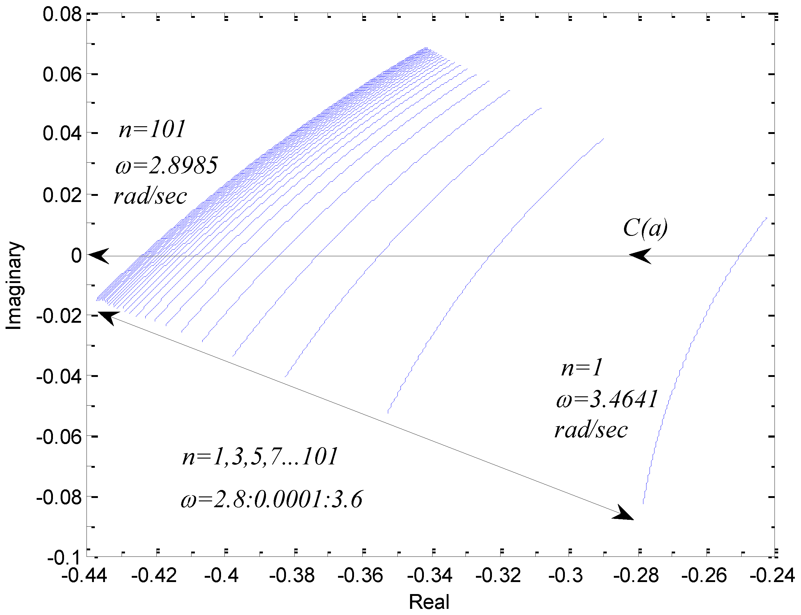
 and G(jω) provides a good graphical approach for obtaining the limit cycle solution. Another option, to obtain the limit cycle frequency, is to solve


| n | ω (rad/s) | n | ω (rad/s) |
|---|---|---|---|
| 1 | 0.6450 | 9 | 0.6359 |
| 3 | 0.6392 | 11 | 0.6357 |
| 5 | 0.6370 | 13 | 0.6356 |
| 7 | 0.6362 | 15 | 0.6356 |


| n | ω (rad/s) | n | ω (rad/s) |
|---|---|---|---|
| 1 | 3.4641 | 17 | 2.9578 |
| 3 | 3.2003 | 23 | 2.9398 |
| 5 | 3.0995 | 35 | 2.9218 |
| 7 | 3.0471 | 51 | 2.9107 |
| 9 | 3.0152 | 71 | 2.9038 |
| 11 | 2.9938 | 91 | 2.8998 |
| 13 | 2.9784 | 101 | 2.8985 |


 . For the transfer function of Equation (41), one can write


3.2.1. Analysis of Limit Cycle Existence According to Compensator Gain


3.2.2. Analysis of Limit Cycle Existence According to Fractional Order Dynamics


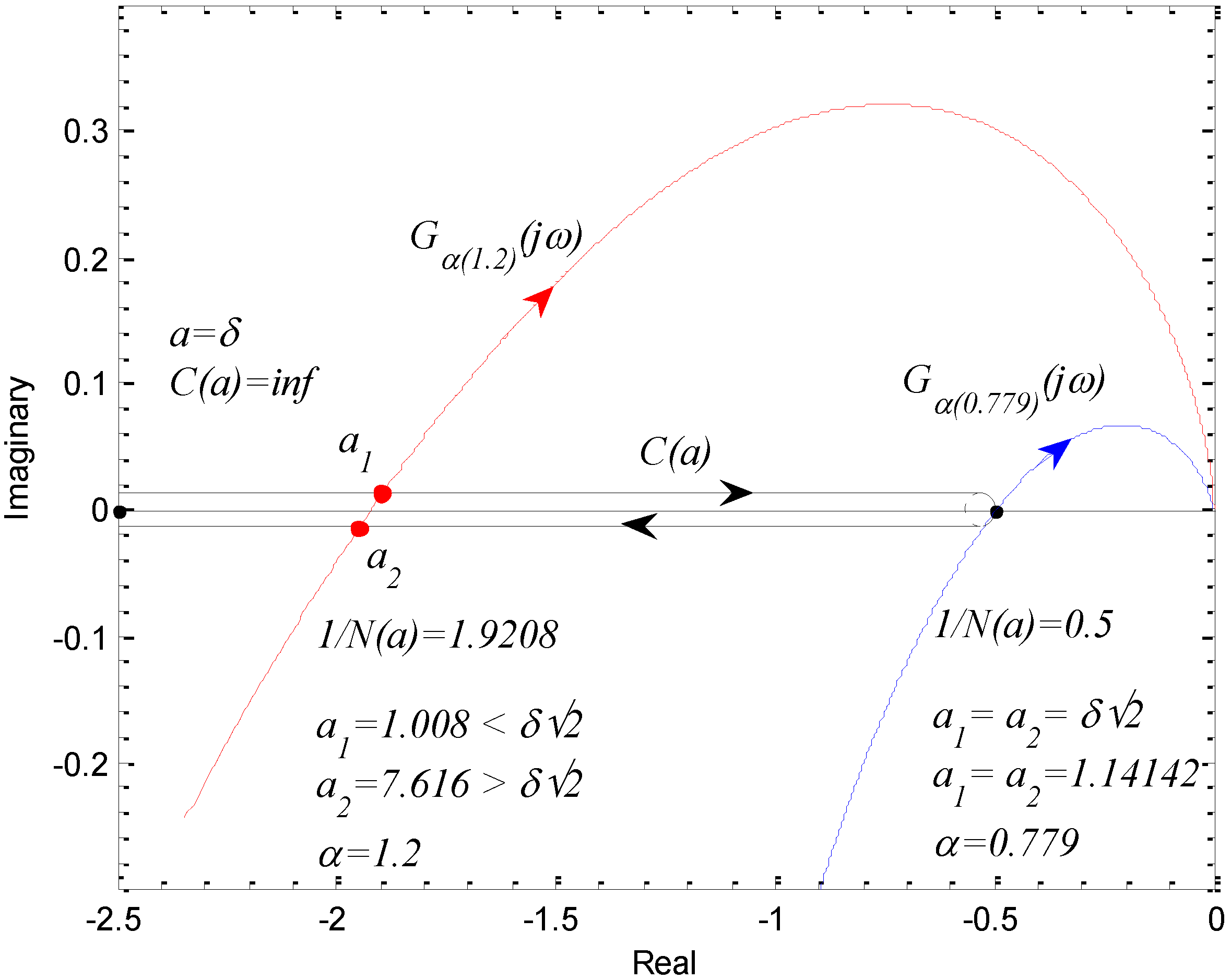
| α (Fractional Order) | ω rad/s (The Frequency at arg[G(jω)] = −π) | a (The Amplitude at arg[G(jω)] = −π) |
|---|---|---|
| 0.779 | 1.4252 | a1 = 1.141, a2 = 1.141 |
| 1.1 | 0.8541 | a1 = 1.0176, a2 = 5.407 |
| 1.2 | 0.7265 | a1 = 1.008, a2 = 7.616 |
| 1.3 | 0.6128 | a1 = 1.004, a2 = 10.946 |
| 1.4 | 0.5095 | a1 = 1.001, a2 = 16.294 |
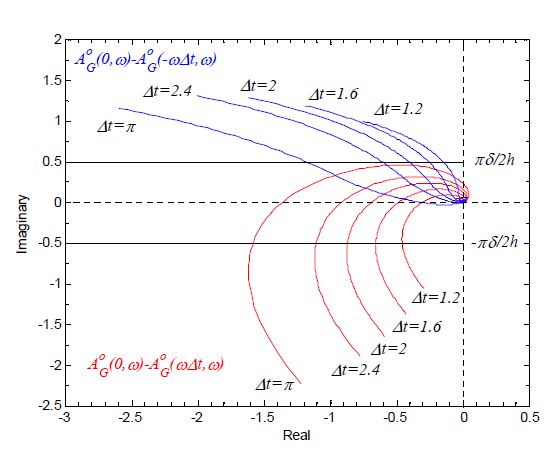
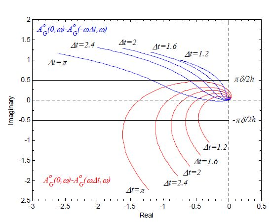
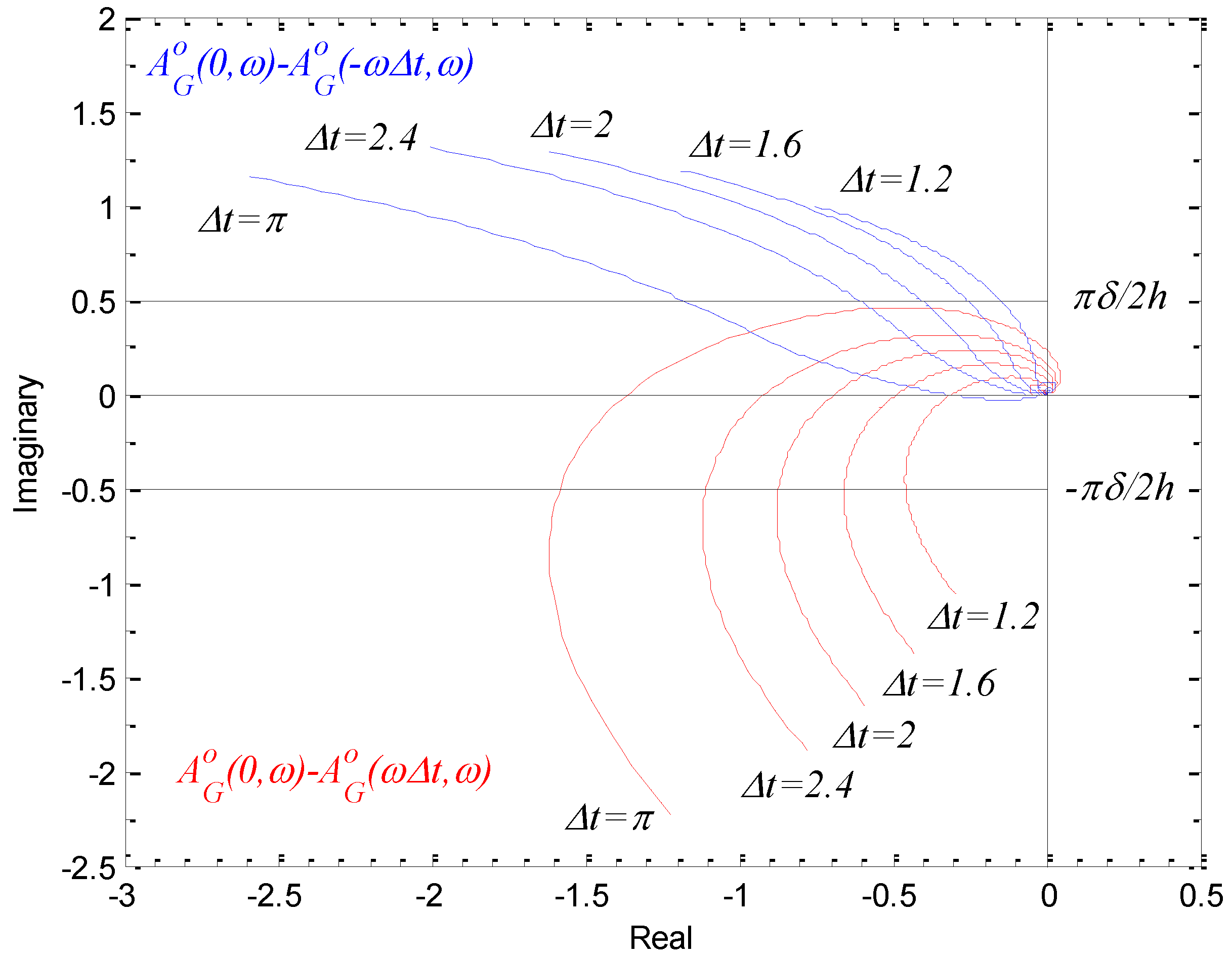
and were plotted for a selection of values of Δt as shown in Figure 26, and the values of ω and Δt were recorded where they met the lines −πδ/2h and πδ/2h, respectively. Table 4 shows recorded values of ω and Δt for K = 1.
| Δt | ω rad/s (Solution from = −πδ / 2h) | ω rad/s (Solution from = πδ / 2h) |
|---|---|---|
| 0.4 | 0.222 | 0.216 |
| 0.6 | 0.577 | 0.61 |
| 0.8 | 0.736 | 0.835 |
| 1 | 0.818 | 0.983 |
| 1.2 | 0.861 | 1.083 |
| 1.4 | 0.881 | 1.146 |
| 1.6 | 0.886 | 1.177 |
| 1.8 | 0.881 | 1.181 |
| 2.0 | 0.871 | 1.165 |
| 2.2 | 0.856 | 1.132 |
| 2.4 | 0.838 | 1.088 |
| 2.6 | 0.82 | 1.037 |
| 2.8 | 0.8 | 0.98 |
| 3.14 | 0.767 | 0.878 |
| 3.2 | 0.761 | 0.859 |
| 3.4 | 0.741 | 0.797 |
| 3.6 | 0.723 | 0.735 |
| 3.8 | 0.704 | 0.673 |
| 4 | 0.687 | 0.612 |
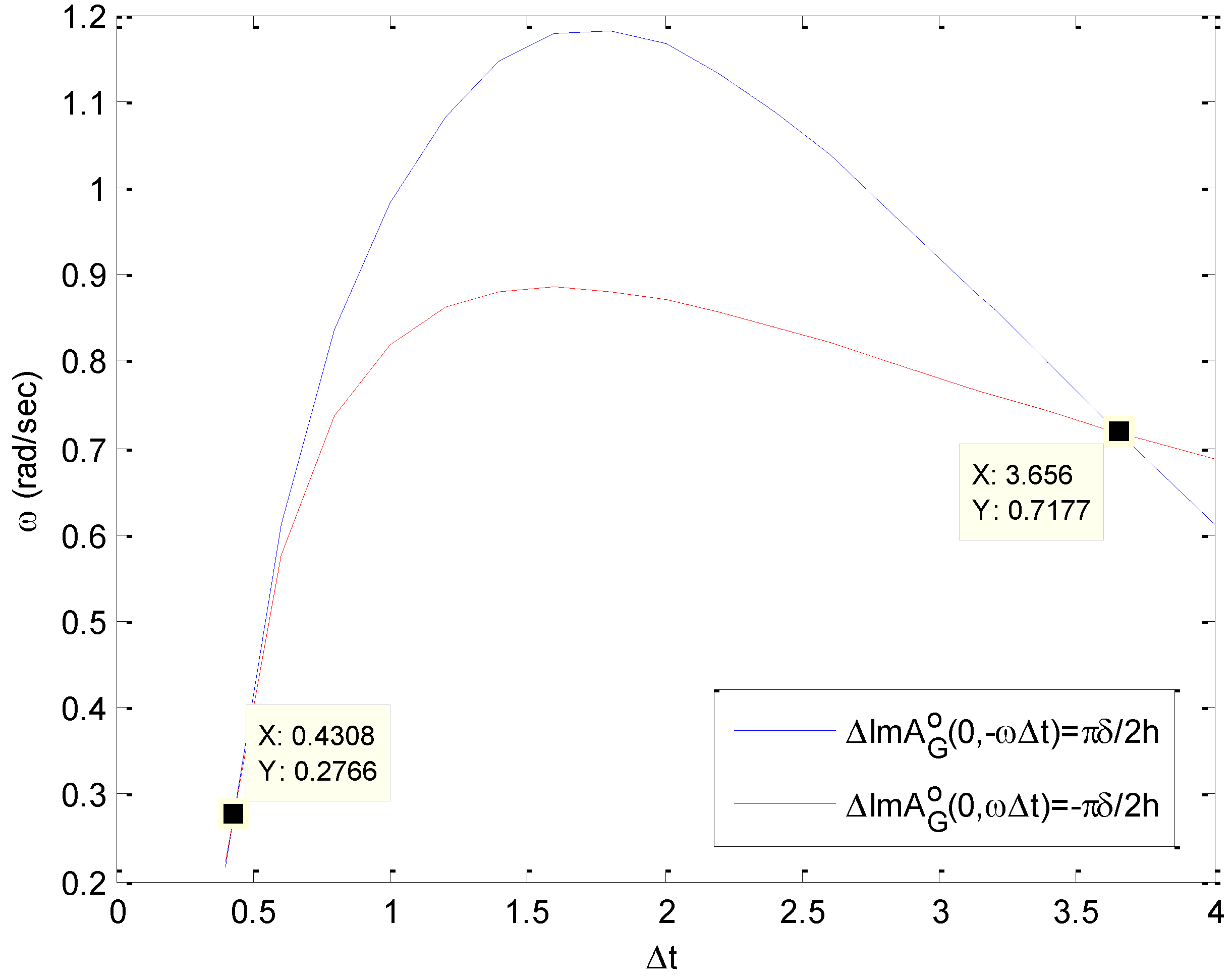
= −πδ/2h and = πδ/2h can then be found by plotting the values given in Table 4 in (Δt, ω ) plane as shown in Figure 27. From Figure 27, it was found that there are two solutions one is (Δt, ω ) = (3.656 s, 0.7177 rad/s) and the other is (Δt, ω ) = (0.4308 s, 0.2766 rad/s).
| K | ω | Δt | θ = ωΔt |
|---|---|---|---|
| 1 | 0.7177 | 3.656 | 2.623 |
| 0.2766 | 0.4308 | 0.119 | |
| 0.6 | 0.7142 | 3.055 | 2.181 |
| 0.5712 | 1.044 | 0.596 | |
| 0.55 | 0.7204 | 2.664 | 1.919 |
| 0.6103 | 1.246 | 0.760 | |
| 0.52 | 0.7152 | 2.438 | 1.7437 |
| 0.6411 | 1.444 | 0.9257 | |
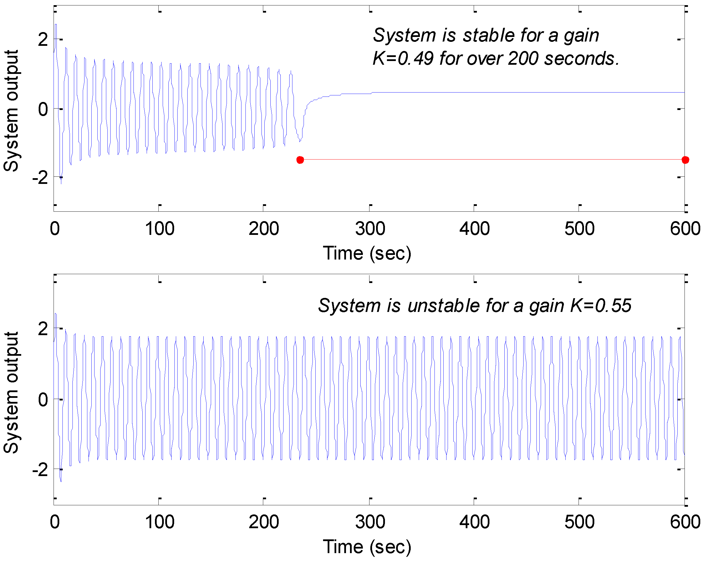
| 0.49 | No solution. System is stable | ||
| K | Method | ω | Δt | θ = ωΔt |
|---|---|---|---|---|
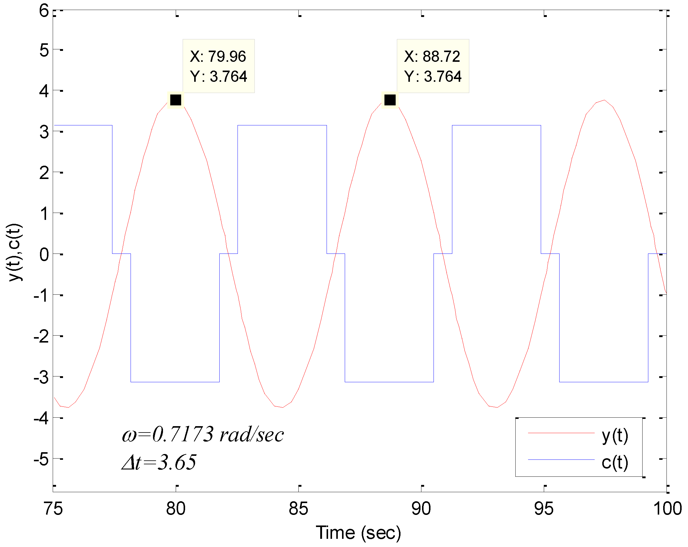
| 1 | Simulation | 0.7173 | 3.65 | 2.618 |
| - | - | - | ||
| DF | 0.7265 | 3.57 | 2.59 | |
| - | - | - | ||
| A Locus | 0.7177 | 3.656 | 2.623 | |
| 0.2766 | 0.4308 | 0.119 | ||
| 0.6 | Simulation | 0.7306 | 2.9 | 2.118 |
| - | - | - | ||
| DF | 0.7265 | 2.88 | 2.09 | |
| - | - | - | ||
| A Locus | 0.7142 | 3.055 | 2.181 | |
| 0.5712 | 1.044 | 0.596 | ||
| 0.55 | Simulation | 0.7222 | 2.7 | 1.949 |
| - | - | - | ||
| DF | 0.7265 | 2.61 | 1.896 | |
| - | - | - | ||
| A Locus | 0.7204 | 2.664 | 1.919 | |
| 0.6103 | 1.246 | 0.760 | ||
| 0.52 | Simulation | 0.7140 | 2.4 | 1.713 |
| - | - | - | ||
| DF | No solution. System is stable. | |||
| A Locus | 0.7152 | 2.438 | 1.743 | |
| 0.6411 | 1.444 | 0.9257 | ||
| 0.49 | Simulation | No limit cycle. System is stable. | ||
| DF | No solution. System is stable. | |||
| A Locus | No solution. System is stable. | |||

4. Conclusions
Author Contributions
Conflicts of Interest
References
- Sun, H.; Song, X.; Chen, Y.Q. A class of fractional order dynamic systems with fuzzy order. In Proceedings of the 8th World Congress on Intelligent Control and Automation, Jinan, China, 6–9 July 2010; pp. 197–201.
- Xue, D.; Chen, Y.Q. A comparative introduction of four fractional order controllers. In Proceedings of the 4th World Congress on Intelligent Control and Automation, Shanghai, China, 10–14 June 2002; pp. 3228–3235.
- Oustaloup, A.; Melchior, P.; Lanusse, P.; Cois, O.; Dancla, F. The CRONE toolbox for MATLAB. In Proceedings of the 2000 IEEE International Symposium on Computer Aided Control System Design, Anchorage, AK, USA, 25–27 September 2000; pp. 190–195.
- Valerio, D.; da Costa, J.S. Ninteger: A non-integer control toolbox for Matlab. In Proceedings of the 1st IFAC Workshop on Fractional Differentiation and Its Applications, Bordeaux, France, 19–21July 2004.
- Tepljakov, A.A.; Petlenkov, E.; Belikov, J. FOMCON: Fractional-order modeling and control toolbox for Matlab. In Proceedings of the 18th International Conference, Mixed Design of Integrated Circuits and Systems, Gliwice, Poland, 16–18 June 2011; pp. 684–689.
- Xue, D.; Chen, Y.Q.; Atherton, D.P. Feedback Control Systems—Analysis and Design with MATLAB 6; Springer-Verlag: London, UK, 2002. [Google Scholar]
- Podlubny, I. Fractional-order systems and PIλDμ controllers. IEEE Trans. Autom. Control 1999, 44, 208–214. [Google Scholar] [CrossRef]
- Sabatier, J.; Poullain, S.; Latteux, P.; Thomas, J.L.; Oustaloup, A. Robust speed control of a low damped electromechanical system based on CRONE control: Application to a four mass experimental test bench. Nonlinear Dyn. 2004, 38, 383–400. [Google Scholar]
- Valério, D.; da Costa, J.S. Time domain implementation of fractional order controllers. IEEE Proc. Control Theory Appl. 2005, 152, 539–552. [Google Scholar]
- Machado, J. Discrete-time fractional-order controllers. Fract. Calc. Appl. Anal. 2001, 4, 47–66. [Google Scholar]
- Monje, C.A.; Vinagre, B.M.; Feliu, V. Tuning and auto-tuning of fractional order controllers for industry applications. Control Eng. Pract. 2008, 16, 798–812. [Google Scholar] [CrossRef]
- Chen, Y.Q.; Ahn, H.S.; Podlubny, I. Robust stability check of fractional order linear time invariant systems with interval uncertainties. Signal Process. 2006, 86, 2611–2618. [Google Scholar] [CrossRef]
- Tan, N.; Ozguven, O.F.; Ozyetkin, M.M. Robust stability analysis of fractional order interval polynomials. ISA Trans. 2009, 48, 166–172. [Google Scholar] [CrossRef] [PubMed]
- Atherton, D.P. An Introduction to Nonlinearity in Control Systems. Ventus Publishing Aps., 2011. Available online: http://bookboon.com/en/an-introduction-to-nonlinearity-in-control-systems-ebook (accessed on 31 March 2014).
- Atherton, D.P. Nonlinear Control Engineering: Describing Function Analysis and Design; Van Nostrand Reinhold: London, UK, 1975. [Google Scholar]
- Atherton, D.P. Stability of Nonlinear Systems; Research Studies Press, John Wiley: Chichester, NH, USA, 1981. [Google Scholar]
- Tsypkin, Y.Z. Relay Control Systems; Cambridge University Press: England, UK, 1984. [Google Scholar]
- Das, S. Functional Fractional Calculus for System Identification and Control; Springer-Verlag: Berlin/Heidelberg, Germany, 2008. [Google Scholar]
- Nonnenmacher, T.F.; Glöckle, W.G. A fractional model for mechanical stress relaxation. Philos. Mag. Lett. 1991, 64, 89–93. [Google Scholar] [CrossRef]
- Westerlund, S.; Ekstam, L. Capacitor theory. IEEE Trans. Dielectr. Electr. Insul. 1994, 1, 826–839. [Google Scholar] [CrossRef]
- Bagley, R.L.; Calico, R.A. Fractional order state equations for the control of viscoelastic structures. J. Guid. Control Dyn. 1991, 14, 304–311. [Google Scholar] [CrossRef]
- Skaar, S.B.; Michel, A.N.; Miller, R.K. Stability of viscoelastic control systems. IEEE Trans. Autom. Control 1988, 33, 348–357. [Google Scholar] [CrossRef]
- Ichise, M.; Nagayanagi, Y.; Kojima, T. An analog simulation of non-integer order transfer functions for analysis of electrode processes. J. Electroanal. Chem. Interfacial Electrochem. 1971, 33, 253–265. [Google Scholar] [CrossRef]
- Hartley, T.T.; Lorenzo, C.F. Dynamics and control of initialized fractional-order systems. Nonlinear Dyn. 2002, 29, 201–233. [Google Scholar] [CrossRef]
- Sun, H.; Abdelwahab, A.; Onaral, B. Linear Approximation of transfer function with a pole of fractional power. IEEE Trans. Autom. Control 1984, 29, 441–444. [Google Scholar] [CrossRef]
- Mandelbrot, B. Some noises with 1/f spectrum, a bridge between direct current and white noise. IEEE Trans. Inf. Theory 1967, 13, 289–298. [Google Scholar] [CrossRef]
- Goldberger, A.L.; Bhargava, V.; West, B.J.; Mandell, A.J. On the mechanism of cardiac electrical stability. Biophys. J. 1985, 48, 525–528. [Google Scholar] [CrossRef] [PubMed]
- Magin, R.L. Fractional Calculus in Bioengineering; Begell House Publishers: CT, USA, 2006. [Google Scholar]
- Hartley, T.T.; Lorenzo, C.F.; Qammar, H.K. Chaos in a fractional order Chua system. IEEE Trans. Circuits Syst. I 1995, 42, 485–490. [Google Scholar] [CrossRef]
- Monje, C.A.; Chen, Y.Q.; Vinagre, B.M.; Xue, D.; Feliu, V. Fractional-Order Systems and Controls: Fundamentals and Applications; Springer: London; New York, 2010. [Google Scholar]
- Podlubny, I. Fractional Differential Equations; Academic Press: San Diego, CA, USA, 1999. [Google Scholar]
- Krajewski, W.; Viaro, U. A method for the integer-order approximation of fractional-order systems. J. Frankl. Inst. 2014, 351, 555–564. [Google Scholar] [CrossRef]
- Vinagre, B.M.; Podlubny, I.; Herńandez, A.; Feliu, V. Some approximations of fractional order operators used in control theory and applications. Fract. Calc. Appl. Anal. 2000, 3, 231–248. [Google Scholar]
- Chen, Y.Q.; Petráš, I.; Xue, D. Fractional order control—A tutorial. In Proceedings of the 2009 American Control Conference, Hyatt Regency Riverfront, St. Louis, MO, USA, 10–12 June 2009; pp. 1397–1411.
- Krishna, B.T. Studies on fractional order differentiators and integrators: A survey. Signal Process. 2011, 91, 386–426. [Google Scholar] [CrossRef]
- Djouambi, A.; Charef, A.; Voda, A. Numerical Simulation and Identification of Fractional Systems using Digital Adjustable Fractional Order Integrator. In Proceedings of the 2013 European Control Conference (ECC), Zürich, Switzerland, 17–19 July 2013; pp. 2615–2620.
- Oustaloup, A.; Levron, F.; Mathieu, B.; Nanot, F.M. Frequency band complex noninteger differentiator: Characterization and synthesis. IEEE Trans. Circuit Syst. I Fundam. Theory Appl. 2000, 47, 25–39. [Google Scholar] [CrossRef]
- Carlson, G.E.; Halijak, C.A. Approximation of fractional capacitors (1/s)1/n by a regular Newton process. IEEE Trans. Circuit Theory 1964, 11, 210–213. [Google Scholar] [CrossRef]
- Matsuda, K.; Fujii, H. H∞-optimized wave-absorbing control: Analytical and experimental results. J. Guid. Control Dyn. 1993, 16, 1146–1153. [Google Scholar] [CrossRef]
- Charef, A.; Sun, H.H.; Tsao, Y.Y.; Onaral, B. Fractal system as represented by singularity function. IEEE Trans. Autom. Control 1992, 37, 1465–1470. [Google Scholar] [CrossRef]
- Duarte, V.; Costa, J.S. Time-domain implementations of non-integer order controllers. In Proceedings of the Controlo 2002, Aveiro, Portugal, 5–7 September 2002; pp. 353–358.
- Ozyetkin, M.M.; Yeroglu, C.; Tan, N.; Tagluk, M.E. Design of PI and PID controllers for fractional order time delay systems. In Proceedings of the 9th IFAC workshop on Time Delay Systems, Prague, Czech, 7–9 June 2010.
- Atherton, D.P. Early developments in nonlinear control. IEEE Control Syst. 1996, 16, 34–43. [Google Scholar] [CrossRef]
© 2014 by the authors; licensee MDPI, Basel, Switzerland. This article is an open access article distributed under the terms and conditions of the Creative Commons Attribution license (http://creativecommons.org/licenses/by/3.0/).
Share and Cite
Atherton, D.P.; Tan, N.; Yeroglu, C.; Kavuran, G.; Yüce, A. Limit Cycles in Nonlinear Systems with Fractional Order Plants. Machines 2014, 2, 176-201. https://doi.org/10.3390/machines2030176
Atherton DP, Tan N, Yeroglu C, Kavuran G, Yüce A. Limit Cycles in Nonlinear Systems with Fractional Order Plants. Machines. 2014; 2(3):176-201. https://doi.org/10.3390/machines2030176
Chicago/Turabian StyleAtherton, Derek P., Nusret Tan, Celaleddin Yeroglu, Gürkan Kavuran, and Ali Yüce. 2014. "Limit Cycles in Nonlinear Systems with Fractional Order Plants" Machines 2, no. 3: 176-201. https://doi.org/10.3390/machines2030176