Automatic Motion Generation for Robotic Milling Optimizing Stiffness with Sample-Based Planning

Abstract

Optimal and intuitive robotic machining is still a challenge. One of the main reasons for this is the lack of robot stiffness, which is also dependent on the robot positioning in the Cartesian space. To make up for this deficiency and with the aim of increasing robot machining accuracy, this contribution describes a solution approach for optimizing the stiffness over a desired milling path using the free degree of freedom of the machining process. The optimal motion is computed based on the semantic and mathematical interpretation of the manufacturing process modeled on its components: product, process and resource; and by configuring automatically a sample-based motion problem and the transition-based rapid-random tree algorithm for computing an optimal motion. The approach is simulated on a CAM software for a machining path revealing its functionality and outlining future potentials for the optimal motion generation for robotic machining processes.

1. Introduction

Robot systems have become more common in industry due to their low cost, flexibility and versatility. However, the main challenge for this technology, in order to also be used massively in machining operations, is its lack of absolute accuracy. One of the factors affecting the absolute positioning accuracy while machining is the lack of robot stiffness, which is the criterion studied and optimized, into a motion planning problem, in this research. Moreover, another extra challenge of robotic machining is the time-consuming, expert-dependent and complex programming process. This publication addresses a method for automatically optimizing robot stiffness by minimizing deviations due to the robot compliance for a machining task using the free degree of freedom of the milling process. Evidence of these challenges is that industrial robots are still not widely used for machining purposes. Proof of that is the IFR statistics. According to the IFR, just two percent of the world estimated annual shipments of industrial robots is related to processing task, and from this two percent, thirty nine percent are dedicated to tasks, such as mechanical cutting, grinding, deburring, milling or polishing [1], which is a smaller quantity taking into account the flexibility and reconfigurability of robot systems. The reasons for addressing optimization and automatic programming are that several advantages could be derived if robots were widely used for machining operations. Some of these reasons are: (1) less work space will be required if robots are used for machining instead of CNC machines; (2) robots are now less expensive than CNC machines and could represent cost savings in industry; (3) robots are more flexible and could also be used for doing other tasks in addition to the machining operation, such as picking the workpiece, if the robot is provided with a tool changer and a gripper, increasing the productivity; (4) the dexterity of the robot could be used more effectively to machine complex machining parts; and furthermore, (5) a robot could substitute heavy manual work, which may be a risk for human health.

Due to the above-mentioned advantages, the demand for quick reconfiguration of robots for precise machining applications has been pointed out as a required strategy for responding to the current demand of product individualization [2]. Three main obstacles, (1) insufficient rigidity, (2) poor accuracy and (3) complex programming, have been identified for the machining of hard materials with robot systems [3]. The complexity of programming has been pointed out as of one of the most important limiting factors [4]. Robot stiffness, vibrations and system natural frequencies are also referred to as critical factors [5]. In conjunction with the identification of limitations, several researchers have also experimentally determined error sources [6] and proposed strategies for improving robotic machining accuracy through modular compensation [7], which could be a way for increasing the robot accuracy and its accurate programmability. In one of our last publications, an error source structure for the identification and model-based compensation of errors in robotic manufacturing has been proposed using the Product, Process and Resource model (PPR) [8]. A comparison between sensor-based and compliance model-based compensation for robotic drilling has been presented [8]. This model has been extended in this publication into an architecture for optimizing robot machining motions optimizing robot stiffness.

In a similar way to the error source identification, several researchers have conducted studies on the modeling of robot compliance for compensating deviations in order to improve accuracy. In one of our previous works, the automatic robot stiffness pose optimization for robotic processes has been presented, and the definition of different criteria, such as end-effector stiffness optimization in process direction, damping, collision and reachability, and the different interpretations for applications, such as drilling, deburring, cutting and milling, have been looked at [9]. Lehmann proposes a three-step approach, machining strategy generation, offline force compensation and online force compensation, as a strategy to compensate the force-induced accuracy influences. Optimization of the parameters, such as workpiece location, eigenfrequencies of the robot and robot structure in given configurations, is pointed out as an important criteria for the machining process [10]. Use of the possible robot configurations for optimizing stiffness is addressed in this research.

Other researchers, such as Tyapin, implement an offline path compensation by using estimated process forces based on a static force model and by computing the deformations also using identified joint stiffness models [11]. As a further strategy to reduce and compensate the process force-induced errors in milling, this author states that “The stiffness of a manipulator depends on the configuration, hence the stiffness could be found in different configurations and interpolation techniques could be used to compute the stiffness in all other configurations” [11], which supports the developed work and the results presented in this publication. Slavkovic models cutting forces and the robot compliance in order to predict the cutting force-induced tool tip displacements for offline compensation of cutting force-induced errors in five-axis robotic machining [4]. Abele predicts the tool displacement for the milling process [12] and also describes a method to predict tool displacement by coupling the elastic serial model with the milling process model [13]. Bauer implements a sensor-based and a model-based compensation for the robot milling process. The model-based compensation uses a robot dynamic model and a milling force model with which the robot deviations due to process forces are computed and compensated [14].

Several methods are found in the literature for the stiffness and compliance modeling. One of them is to identify stiffness by the clamping method, in which the robot is locked in a closed kinematic loop and then exercises joint-based movements while sensing motor position and torque [15]. The identification of the diagonal joint stiffness matrix is also approached by applying external wrenches [16]. The stiffness modeling of heavy industrial robots with gravity compensators has also been studied [17]. 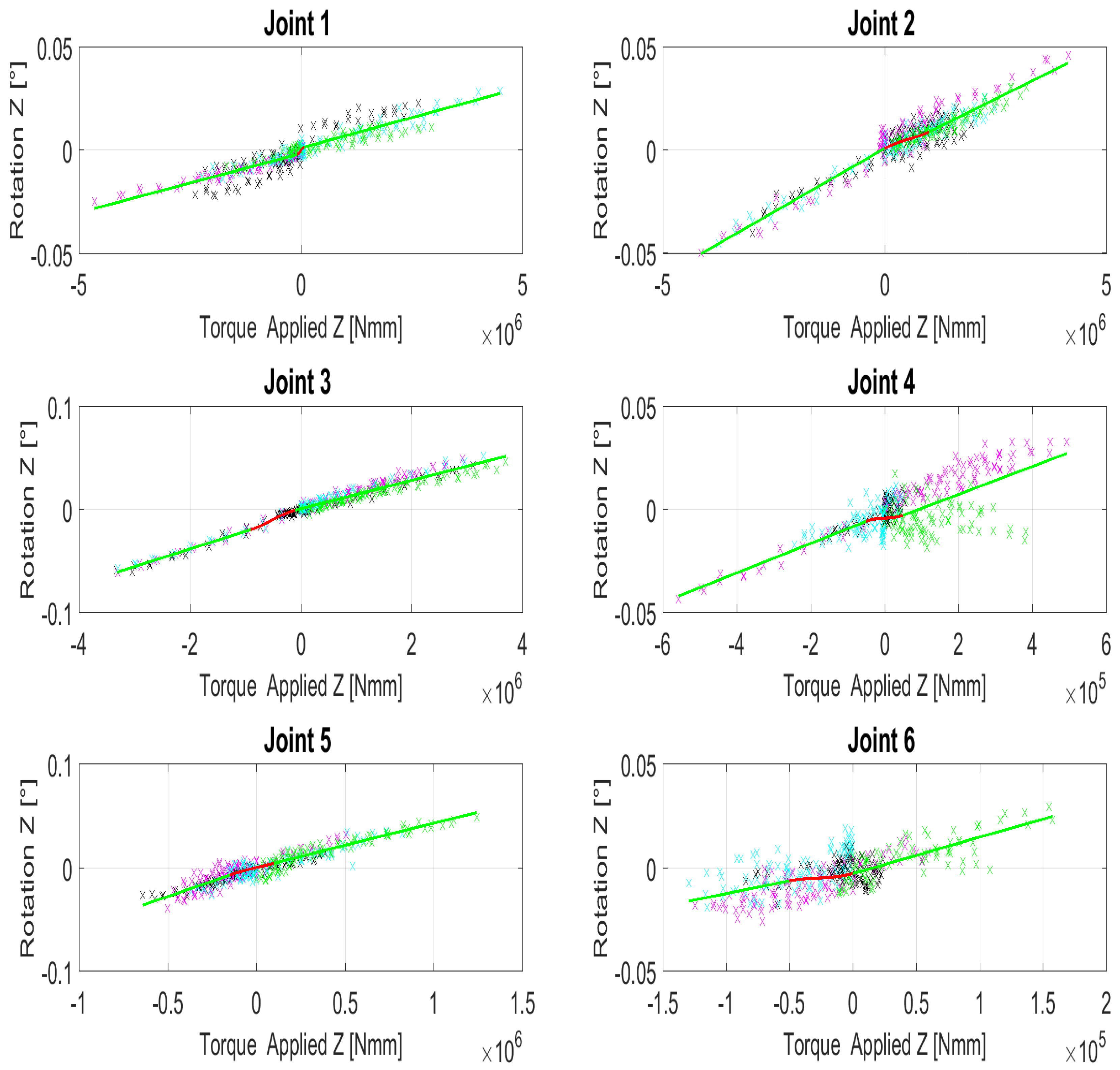The calculation of the Cartesian stiffness based on the polar stiffness and the use of the Jacobian matrix has also been proposed as a modeling alternative [18]. The robot stiffness used in this contribution is identified as linear descriptions on the ranges where no backlash is observed and nonlinear functions are addressed when gear deformation is noticed [9].

The study of stiffness is also used in control for compensating errors. Pan and Wang introduced an online deformation compensation approach based on a robot structure model for controlling the material removal rate. This approach controls the machining force by adjusting the robot feed speed in real time for improving part quality [19,20,21]. Conclusions from Pan and Wang determine that “The pattern of the process structure deformation is related to all of the following parameters: robot configuration, the location in the workspace, and the direction as well as the magnitude of the process force” [20], depicting the relevance to optimize robot configurations in relation to the robot stiffness. Liu proposes an adaptive control constraint of machining processes with a constant cutting force control system [22]. Olof ensures time-efficiency and improves the accuracy of robotic machining processes by removing the maximum amount of material per time unit by adaptively controlling the applied force, as well as continuously compensating for the path deviations caused by process forces [23]. The methods used in this publication for identifying robot joint stiffness have also been tested using control structures for improving machining accuracy [24]. Other controls without compliance models, such as the position control of industrial robots using the optical measurement system for machining purposes, have been proposed for improving accuracy [25].

Even though several research works have been conducted on error source identification and classification, robot joint compliance modeling and model-based compensation, only a few studies are to be found regarding optimization in this area. One work related with optimization is the one of Dumas in which a workpiece positioning optimization problem using the kinematic redundancy of the milling process is described. For solving this problem, the constraints and the optimization problem are defined and solved with required human intervention using the MasterCAM software for two different workpiece positions predefined in the workspace [26].

As in the last mentioned study, CAM software is now widely used in machining operations. Moreover, it has also been used for compensating deviations. Haage presents a compensation method for increasing robotic machining accuracy using offline compensation computed based on a robot kinematics, a process force and a dynamic robot model used to calculate the compensations embedded into the PowerMill Tool. Results demonstrate more prominent deviations on the corners of a 2D machined rhombus with maintained orientation (without using the DoF of the process) during machining [15]. The combination of holistic programming in CAM software in which the optimization of the redundancy could be used in conjunction with kinematic parameter optimization for optimizing robot machining has also been pointed out [27].

In addition to the software packages, compliance models, identification methods and research on robot accuracy, different sorts of models are available for the machining process itself. For instance, Matsuoka investigates the relationship between the feed rate and the cutting force with an industrial robot and a high speed spindle [28]. Budak introduces a maximization of the chatter free material removal rate in milling by selecting in an optimal way not just the axial, but also the radial depth of cut pairs, which reduces the machining time [29]. Several standards are also available, derived from the CNC machines and machining standards.

Further to the state of the art with respect to robot joint compliance modeling and compensation, other areas in the robotic community have emerged as solutions for the computation of motions. Today, the motion planning algorithm, such as the sample-based technique, is used as an efficient solution to the complex motion problems of robots [30,31,32]. Several applications could be solved with those techniques [33]. However, the motion planning for machining operations has not been studied even though those algorithms are now also available in open-source software [34].

Even with the representative advance in areas such as robotics and CAM simulation, the motion generation for robotic machining (i.e., milling) still presents some challenges. One of these challenges is that the configuration and robot programming of a robotic machining cell are still expert dependent, meaning that qualified personnel with experience in machining operations and robot programming is always required. Moreover, the optimization of the machining processes is mainly achieved due to manual intervention on the generation of programs, using for instance the teach-in approach, and it is case specific. These challenges arise mainly due to the deficiency that machining process characteristics are not directly related to robot motions.

Taking into account the previous problem definition, the need to increase robot accuracy while machining, the benefits of optimizing stiffness based on the robot configuration and the state of the art confirms the need for improvement in the area of robot machining. This research proposes an automatic and intuitive method for optimizing stiffness in the robotic milling process. The document describes the methodology and architecture for automatically computing stiff motions for an industrial robot given a task definition for a robotic milling processes, which is one of the ways in which robots could improve accuracy. This research approaches the optimization problem of the kinematic redundancy of the milling process, automatically defines and configures the required spaces interpreting the constraints and DoF of the product and process for computing, also in an automatic way, a stiff robot motion. The contribution of this research is a clear structure and methodology for modeling a robotic milling process, done based on the PPR process, and the definition of the automatic configuration for state of the art sample-based motion generation algorithms based on the semantic description of the RMP. The approach has been tested and evaluated in a developed CAM software, which uses as input state of the art formats used in CAM simulations.

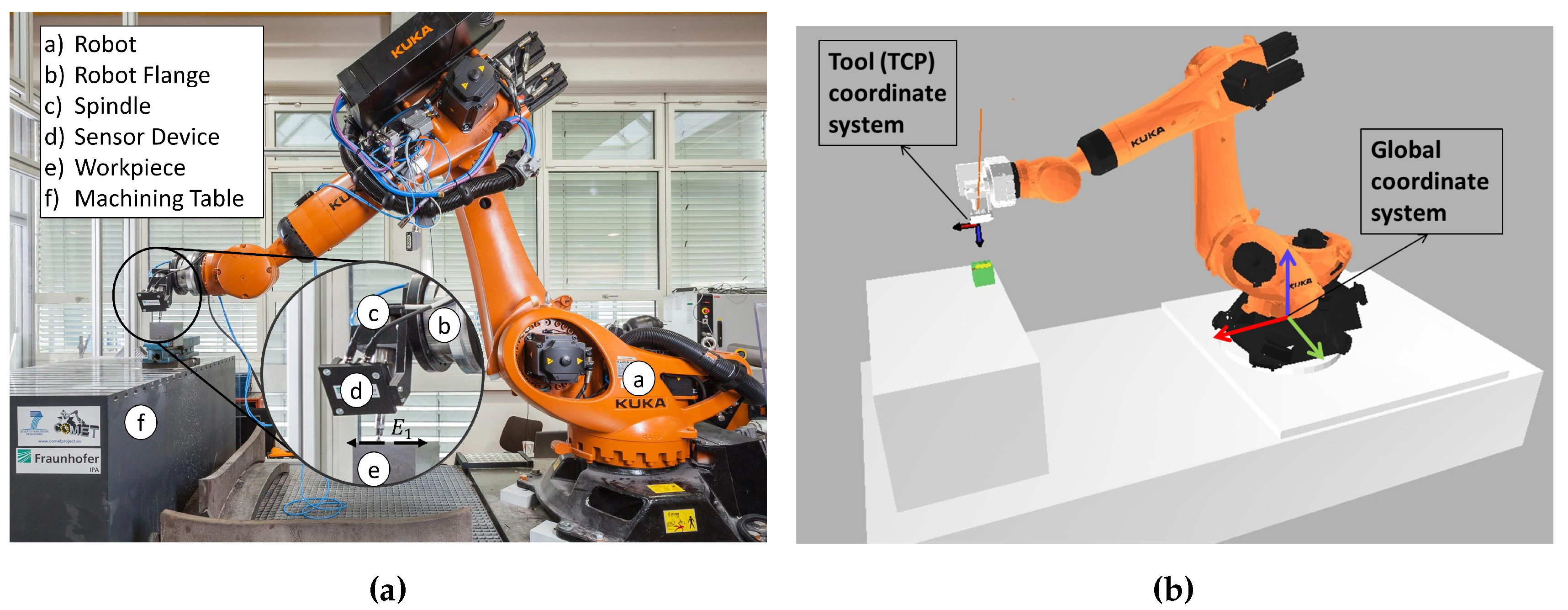
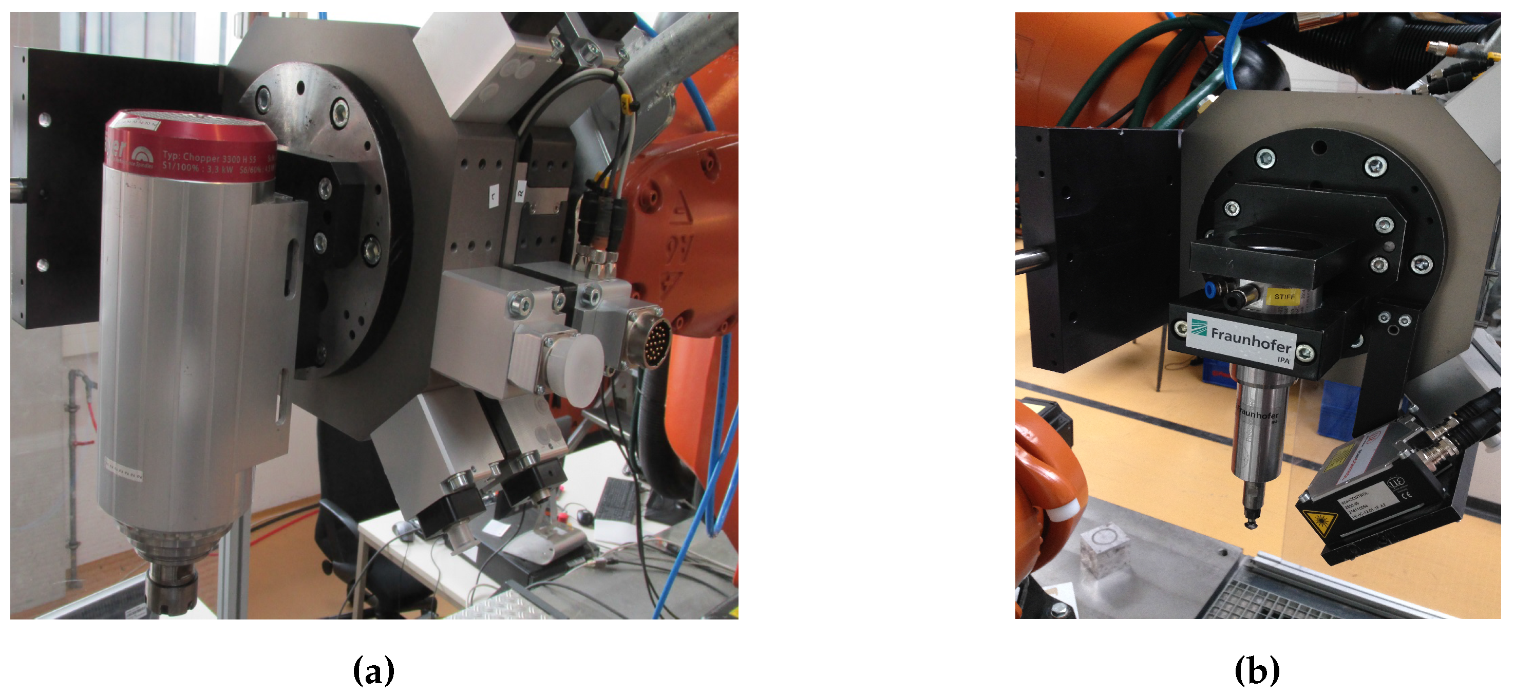
This contribution is organized as follows: Section 2 defines the problem of motion generation for optimizing robot stiffness in machining processes. Section 3 describes the robot cell in which the optimization and evaluation is performed. Section 4 outlines the modeling of the Product, Process and Resource (PPR) model. The PPR model is used as the input in the interpretation and automatic configuration of the motion problem further described in Section 5. Section 6 illustrates the experimental simulation and evaluation of the stiff optimized motion planner in the robotic milling process. Finally, the conclusions and potentials are discussed in Section 7.

2. Problem Definition and Methodology

To address improvements in robotic machining accuracy, the following motion problem is defined: compute automatically and offline a feasible and optimal motion σ optimizing the stiffness of the robot $f_{stiff}={\left(f_{compl}\right)}^{-1}$ by using the free degree of freedom of the rotation around the tool axis $\delta \alpha$ throughout all of the path and its initial and final configuration. The optimal motion should take into account the specified end-user task definition and has as inputs a defined world W, in this case the Cartesian space $W=\mathbb{SE}3$, in which the $Product$, $Process$ and $Resource$ $\left(PPR\right)$ components are defined by models (refer to Section 4).

The above defined problem is solved by using the following methodology: First, interpret the $PPR$ model with respect to the optimal motion criteria, in this case the optimization of robot stiffness by minimizing deviations due to the robot compliance, in conjunction with a simplification of the configuration space in which this motion should be computed. Second, configure automatically a state of the art optimal sample-based motion algorithm, including its state validity definition and the state and motion cost functions. Third, compute an optimal motion for parsing it automatically into a robot program, which optimizes the robot stiffness. Similar architecture and methodology have been proposed for optimal collision avoidance in robotic welding in previous publications [35]. 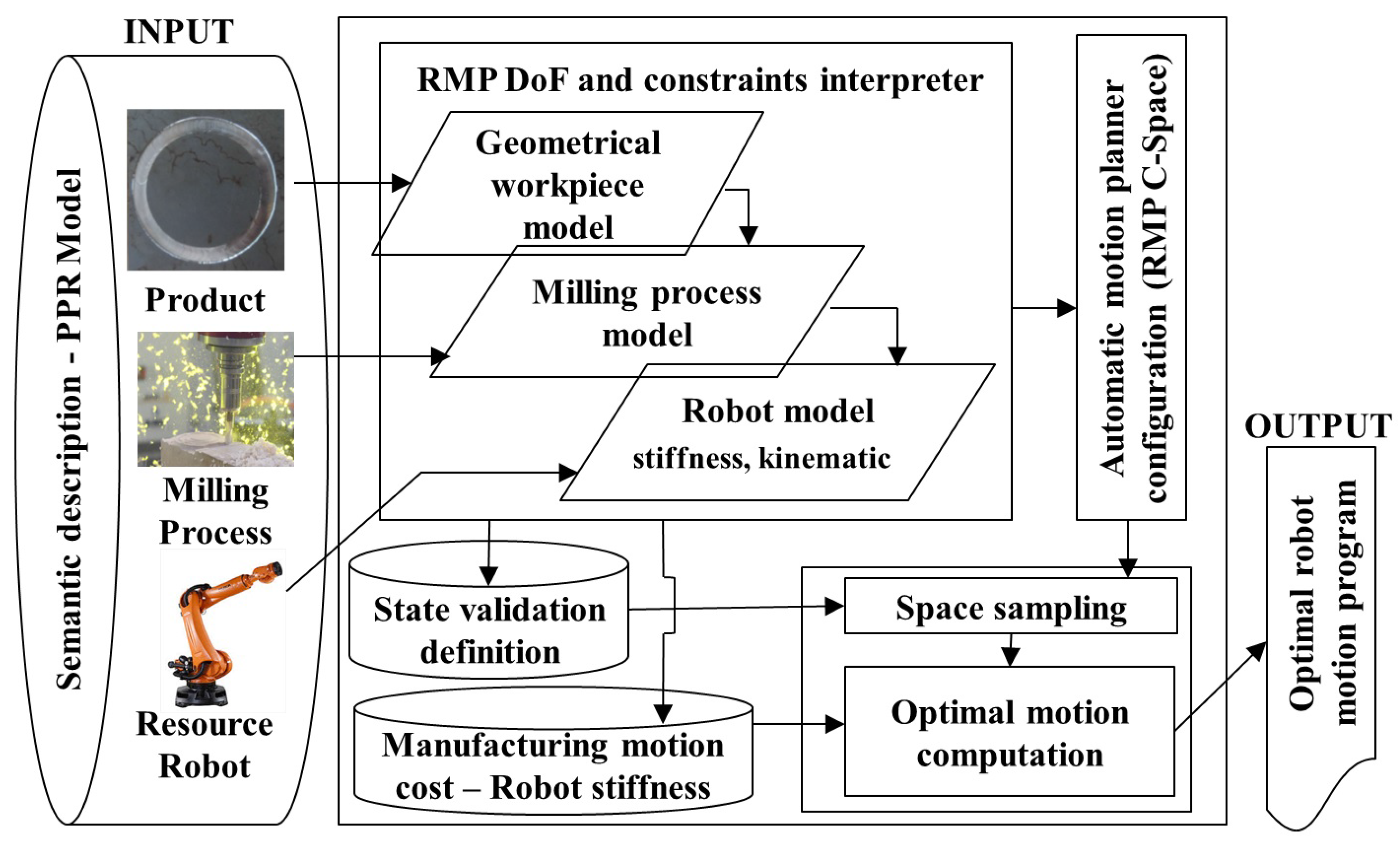Figure 1 depicts the proposed architecture used in order to solve the stiffness optimization motion problem.

For computing a robot milling motion optimizing the robot stiffness, the approach proposes the simplification of the Cartesian space into a new C-space (denominated by the robot manufacturing process configuration space ($\mathbb{RMP}$), in addition to the Cartesian space (defined as $\mathbb{SE}\left(3\right)$) and the joint space (notated as $\mathbb{J}$). The functionality of this new space is to relate motions with the product, process and resource components of the robotic milling process.

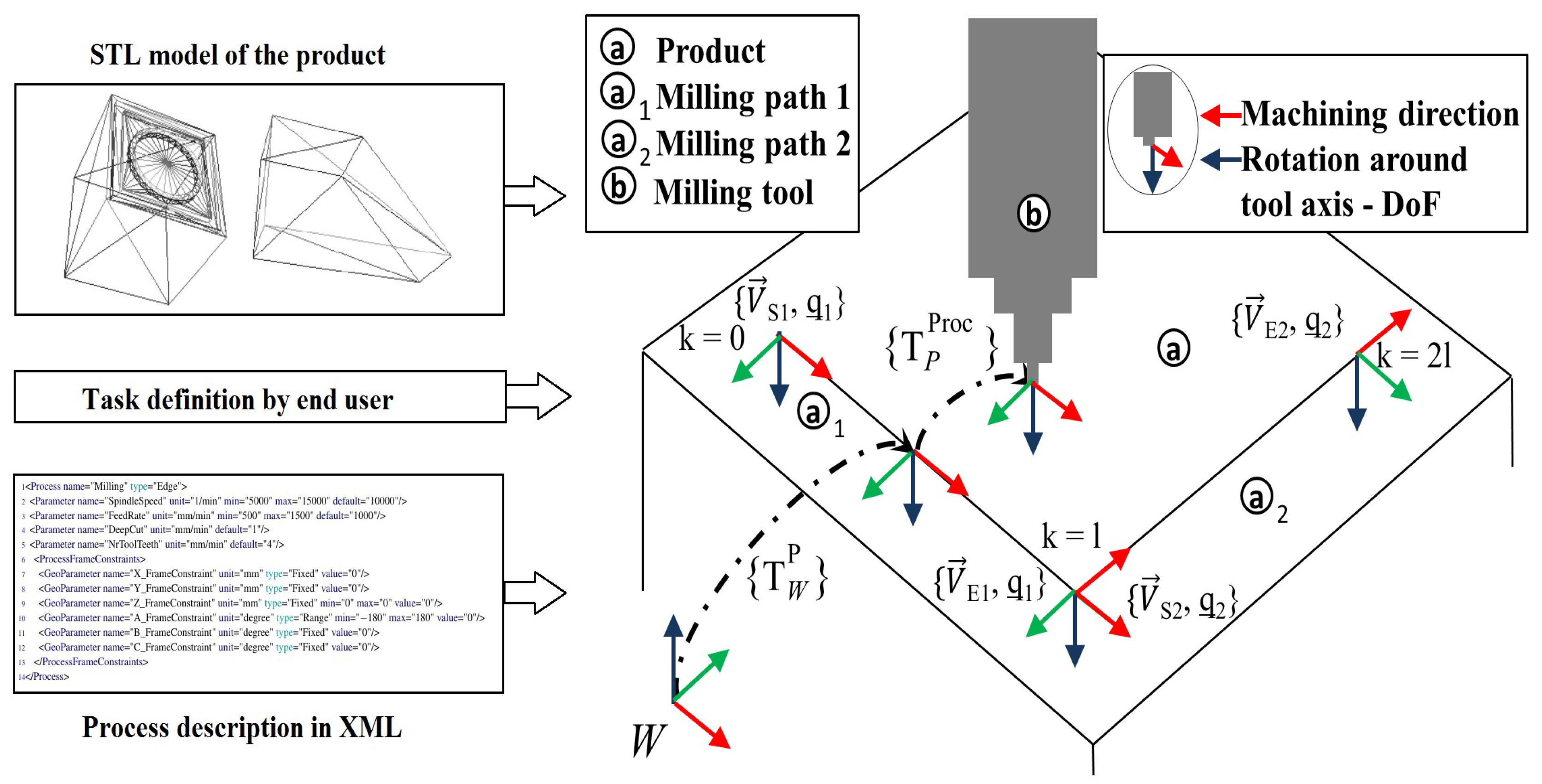
The main goal of the inclusion of this space is the simplification of the manufacturing process. This simplification is achieved by methodologically and automatically transforming the constraint of the product into a DoF and by interrelating it with the DoF of the product, which is specified by the end-user in the semantic description of process parameters and which for this process is the rotation around the tool axis (refer to Section 4.2). The constraint of the product for the milling process is the path in which the milling needs to be performed. 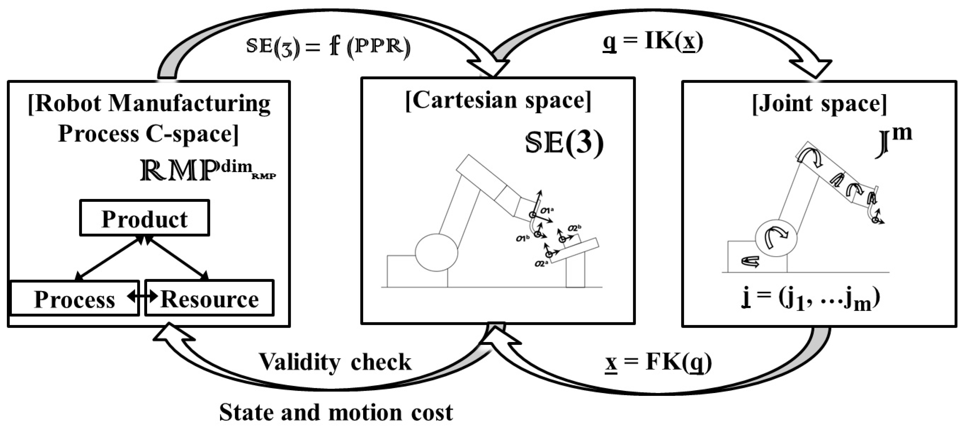Figure 2 shows the involved spaces in the approach. The simplification of the Cartesian space in relation to the milling process is required in order to reduce the computational requirements of the space sampling process required by the sample-based motion algorithms.

The transformation from the robot manufacturing process configuration space to the Cartesian space is notated as $f:PPR\to \mathbb{SE}\left(3\right)$. This transformation is automatically computed, and its computation is described in detail in Section 5.1. Thanks to this transformation, the sample-based motion planning algorithm has the option to evaluate the validity of states and motion costs into $\mathbb{SE}\left(3\right)$, which are retrieved back to the planner for allowing proper and optimal motion planning.

3. Experimental Setup and Simulation

The robotic machining system consists of a Kuka Quantec KR270 2700 ultra industrial robot manipulator, an end-effector with a Chopper spindle tool reference 3300 H S5 from the company Alfred Jäger GmbH (Ober-Mörlen, Germany) (refer to Figure 3a), and a second end-effector with a 2D laser scanner reference scanControl 2900-50 from the company Micro-Epsilon (Ortenburg, Germany) (refer to Figure 3b). A RSP tool changer reference TC 480-1 is used to exchange the end-effectors. The robot is mounted in a machine bed with a table and a mechanical gripping system to hold the workpiece. Figure 4a depicts the described components.

The laser scanner is used in the experimentation (refer to Section 6.2) in order to localize the workpiece in the work-cell. The workpiece CAD model is used to generate a corresponding reference point cloud in order to locate the workpiece using the generalized Iterative Closest Point algorithm (ICP) by comparing the reference with a point cloud obtained with the sensor [36,37]. For automatically generating the stiffness optimized robot program for the machining process, the cell has been modeled in an internally-developed CAM software in which the presented optimization has been implemented. The simulation for this robot is depicted in Figure 4b.

4. Product, Process and Resource Modeling for Robot Milling

The following section describes the models for the components of the product, process and resource architecture, which are the inputs required for the automatic interpretation and configuration of the motion planner (refer to Section 5).

4.1. Product Model

The product model, notated as (P), consists of the mathematical description using homogeneous transformations (notated as T) of single or multiple continuous milling paths of a workpiece. The milling paths are selected by the end-user with a click using the simulation environment, determining in this way the task specification of the process. The end-user determines with the clicks the sequence of the machining. The software has been developed for allowing the modification of the machining direction of a selected machining path in the workpiece.

The description of the translational component of the homogeneous transformation consists of parameterized linear equations (with k as parameter) on the Cartesian space by having as the input the start and end point $\overrightarrow{V}$ of each of the milling paths ${\overrightarrow{V}}_{{\overrightarrow{S}}_n}$ and ${\overrightarrow{V}}_{E_n}$, respectively, where n describes the numbers of selected continuous milling paths by the end-user on the CAM simulation. Each milling path, modeled with the parameterized line equation, is parameterized taking into account the constant $l\in {\mathbb{N}}_{>0}$ being a positive natural number. This constant determines the normalization factor of the length of each edge. In the optimization performed in the CAM software, this constant has been defined as 100. This constant could be adapted in software if required.

The rotational component of the milling path is modeled by obtaining a quaternion notated as ${\underline{q}}_n$. This quaternion is computed taking the direction vector of the machining process as the x vector of the coordinate system (red vectors depicted in Figure 5) and the z vector as the direction in which the milling tool points (blue vectors depicted in Figure 5). The function $R_q$ is defined for computing a rotation matrix having as the input a quaternion. Figure 5 depicts the product model and its notations. Algorithm 1 describes the automatic interpretation for a single or multiple-continuous milling path. The output of Algorithm 1 is the transformation world to product $T_W^P\left(k\right)$ parameterized in k notated with Equation (1). The algorithm is implemented in Python and its output is an equation in C language which is linked to the motion planner. The DoF of the product (notated $Do{F}_p$) is then k and for the model studied in this research of one dimension. The minimum and maximum bounds of the product model are defined as $k_{min}=k_{ini}=0$ and $k_{max}=k_{goal}=nl$, where $nl$ represents the number of selected edges multiplied by the constant, which parameterizes an edge. These bounds are used later on by the motion planning algorithm (refer to Section 5.4).

Algorithm 1 Algorithm for automatic interpretation of the multiple seam product model.
Require: $({\overrightarrow{V}}_{S_1}...{\overrightarrow{V}}_{S_n})$, $({\overrightarrow{V}}_{E_1}...{\overrightarrow{V}}_{E_n})$, $({\underline{q}}_1...{\underline{q}}_n)$, n, l
1:	$T_W^P\left(\begin{array}{c}Do{F}_p\end{array}\right)=T_W^p\left(k\right)=$
2:	$\left[\begin{array}{cc}{R}_q({\underline{q}}_1)& {\overrightarrow{V}}_{S_1}+(\frac{k}{l})({\overrightarrow{V}}_{E_1}-{\overrightarrow{V}}_{S_1})\\ 0& 1\end{array}\right],k\in [0,l]$
3:	if $n>1$ then
4:	for $m=2$ to n do
5:	$\left[\begin{array}{cc}{R}_q({\underline{q}}_m)& {\overrightarrow{V}}_{S_m}+(\frac{k}{l})({\overrightarrow{V}}_{E_m}-{\overrightarrow{V}}_{S_m})\\ 0& 1\end{array}\right],k\in ((m-1)·l,m·l]$
6:	$m=m+1$
7:	end for
8:	endif
9:	return $T_W^p\left(k\right)$	$$\left(1\right)$$

4.2. Process Model

The milling process model ($proc$) is geometrically defined with a homogeneous transformation notated as $\left(T_p^{proc}(·)\right)$, meaning the transformation from product to process, using the Euler convention, which is more intuitive for the end-user when defining constraints and free DoFs of the milling process. Figure 5 depicts this transformation, and Equation (2) notates this transformation. The process description is performed locally, meaning with respect to the coordinate system of the machining path in the workpiece. Position and rotational constants ${(x,y,z,\alpha ,\beta ,\gamma )}_{proc}$ for this transformation are null values because the tool needs to satisfy the constraint of the product milling path. The DoF of the process in this case $Do{F}_{proc}$ is defined as $\delta \alpha$, which is the rotation around the tool axis (z axis of the tool coordinate system as in Figure 5; the RGB convention red, green, blue for x, y and z is used through all of the document). Figure 5 depicts the inputs required for interpreting the conventions introduced in this and in the last subsection.

$$T_p^{proc}\left(\begin{array}{c}Do{F}_{proc}\end{array}\right)=T_p^{proc}{\left(\delta a\right)}_{proc}=\left[\begin{array}{c}{R}_{eul}{\left(\begin{array}{c}\alpha +\delta \alpha \\ \beta \\ \gamma \end{array}\right)}_{proc}{\left[\begin{array}{c}x\\ y\\ z\end{array}\right]}_{proc}\\ 0& 1\end{array}\right]\begin{array}{c}\\ \\ \\ .\end{array}$$

(2)

The definition of the process model parameters is done in an XML file similar to that in [38]. In this XML file, the process parameters are specified, and the degrees of freedom for the process frame are defined for each translation and rotation. Listing 1 depicts the semantic model of the milling process in the XML format with some parameters, such as spindle speed, feed rate, depth of cut, number of tool teeth and the process frame characteristics. From this file, the maximum and minimum of variation for each component of the process frame could be read. For the milling process, the minimum $\delta {\alpha }_{min}$ and maximum $\delta {\alpha }_{max}$ of rotation around the tool axis are defined. The minimum and maximum of rotation for the milling process are defined taking into account that we have a complete degree of freedom over the vector in which the milling tool points (vector z). Other parameters for the robot and the file of the product are linked using the AutomationMLformat similar to that in [39].

Listing 1: Semantical modeling of the milling parameters in XML format.
1	<Process name=“Milling” type=“Edge”>
2	<Parameter name=“SpindleSpeed” unit=“1/min” min=“5000” max=“15000” default=“10000”/>
3	<Parameter name=“FeedRate” unit=“mm/min” min=“500” max=“1500” default=“1000”/>
4	<Parameter name=“DeepCut” unit=“mm/min” default=“1”/>
5	<Parameter name=“NrToolTeeth” unit=“mm/min” default=“4”/>
6	<ProcessFrameConstraints>
7	<GeoParameter name=“X_FrameConstraint” unit=“mm” type=“Fixed” value=“0”/>
8	<GeoParameter name=“Y_FrameConstraint” unit=“mm” type=“Fixed” value=“0”/>
9	<GeoParameter name=“Z_FrameConstraint” unit=“mm” type=“Fixed” min=“0” max=“0” value=“0”/>
10	<GeoParameter name=“A_FrameConstraint” unit=“degree” type=“Range” min=“−180” max=“180” value=“0”/>
11	<GeoParameter name=“B_FrameConstraint” unit=“degree” type=“Fixed” value=“0”/>
12	<GeoParameter name=“C_FrameConstraint” unit=“degree” type=“Fixed” value=“0”/>
13	</ProcessFrameConstraints>
14	</Process>

4.2.1. Process Force Calculation

The process model also specifies the process-dependent parameters that are used to estimate the forces experienced by the robot end-effector during the end milling process. The process parameters are interpreted by the motion planner to in turn estimate the deviation of the robot position in Cartesian coordinates. Process-dependent parameters of end milling are dictated by the standard of DIN844. DIN 844 specifies the feed per tooth $\left(f_z\right)$ in mm/teeth and also the cutting speed $\left(V_C\right)$ in m/min. The cutting parameters, such as the feed rate of the tool and the spindle speed, can be calculated by the standard methods specified in [40]. The feed rate $V_f$ of the tool is calculated using the standardized equation $V_f=n·z·f_z$ where the speed of rotation of the spindle can be calculated by $n=\frac{1000·V_c}{d·\pi }$ in which n is the spindle speed in rpm, z is the number of cutting teeth, $V_f$ is the feed rate in mm/min and d is the diameter of the tool in mm.

The above calculated parameters are used to estimate the process force by using the equation specified in [40]. The forces are calculated using the following equation $F_{Proc}=a_p·h_m·K_c$ [40]; where $h_m$ is the chip size, which is calculated by $h_m=\frac{{360}^{\circ }}{\pi \Delta {\varphi }^{\circ }}\left(\frac{a_e}{d}\right)f_z$ [40], and where $\Delta \varphi$ is the entry angle and is calculated by $cos\Delta \varphi =1-\frac{2a_e}{d}$ [40]. Here, $a_e$ is the depth of cut in mm; d is the diameter of the tool in mm; and $Kc$ is the material-specific cutting coefficient specified by standard in [40] and $a_p$ the cutting width in mm.

4.3. Resource Model: Robot

This subsection describes the models of the resource component, in this case, an industrial robot notated as r with a mounted milling tool on its end-effector as described in Section 3. These models consist of the robot forward and inverse kinematics, the wrench computations in joint space and the robot joint compliance models.

4.3.1. Forward and Inverse Kinematics

The inverse kinematics is defined as $\underline{q}=IK\left(\underline{x}\right)$ in which $\underline{x}={[x,y,z,\alpha ,\beta ,\gamma ]}_{robot}$ defines a pose of the TCP in $\mathbb{SE}\left(3\right)$ with x, y and z as the translation and α, β and γ as the rotation around the translation components, respectively. ${\underline{q}}_{\left[jx1\right]}$ represents the robot joint positions in $\mathbb{J}$ (where j symbolizes the number of robot joints). Each joint frame is notated with q following the number referring to the joint. The forward kinematics is defined as $\underline{x}=FK\left(\underline{q}\right)$.

The robot parameters for describing the robot kinematics have been defined based on the information provided in the robot datasheet. Rotations of joint frames are described around the z axis.

4.3.2. Wrench Computation in Joint Space Due to Process and Joint Weights

The wrench in coordinate system $\mathit{A}$ is defined as the tuple composed of the force and moment as follows $\left({\underline{\omega }}_A\right)={[F,\tau ]}^T$, where $F={[F_x,F_y,F_z]}^T$ represent the forces and $\tau ={[{\tau }_x,{\tau }_y,{\tau }_z]}^T$ the moments in the x, y and z directions of frame $\mathit{A}$. For computing the wrenches, which are required for the state cost evaluation (refer to Section 5.2), the process force and joint masses with its center of masses have been taken into account. The evaluation of process force is described in Section 4.2.1 and the estimation of masses and the center of masses in Appendix A.

The wrench of each joint (frame A) is computed using the transformation from its following joint or coordinate system where forces or moments are applied (frame B) with the force-moment transformation $\left(Tw\right)$, where R represents the rotation matrix and $\mathit{V}$ the translation vector as follows:

$$\underline{{\omega }_A}=\left[\begin{array}{c}{F}_A^A\\ {\tau }_A^A\end{array}\right]=\left[\begin{array}{cc}{R}_B^A& 0\\ {\mathit{V}}_{B_{ORG}}^A\times R_B^A& R_B^A\end{array}\right]\left[\begin{array}{c}{F}_B^B\\ {\tau }_B^B\end{array}\right]=T{w}_B^A\left(\underline{{\omega }_B}\right)=T{w}_B^A\left(\left[\begin{array}{c}{F}_B^B\\ {\tau }_B^B\end{array}\right]\right)$$

(3)

For Joint 6, the computed milling force is mapped from the calibrated TCP frame $\left(tcp\right)$ to the defined joint frame. Moreover, the weight of the end-effector ${\mathit{M}}_{EE}$ is mapped to the joint frame taking into account the center of mass (notated as $cm$ followed by the respective joint indicator) of Axis 6 relative to its frame. Other wrenches for each joint due to joint masses (notated as ${\mathit{M}}_q$ with the respective joint indicator) are computed in the same way. The procedure to estimate the values of the robot joint weights and its center of masses is explained in Appendix A. All joint weights have been defined in the negative z direction in the global coordinate system depicted in Figure 4b. Equation (4) describes the computation of wrenches for a six-joint articulated robot for static poses.

$$\begin{array}{cc}& \underline{{\omega }_{q6}}=T{w}_{tcp}^{q6}\left({[F_{Proc},0]}^T\right)+T{w}_{cm6}^{q6}\left({[{\mathit{M}}_{q6},0]}^T\right)+T{w}_{cmEE}^{q6}\left({[{\mathit{M}}_{EE},0]}^T\right)\hfill \\ & \underline{{\omega }_{q5}}=T{w}_{q6}^{q5}\left({\omega }_{q6}\right)+T{w}_{cm5}^{q5}\left([{\mathit{M}}_{q5},0]\right)\hfill \\ & ⋮\hfill \\ & \underline{{\omega }_{q1}}=T{w}_{q2}^{q1}\left({\omega }_{q1}\right)+T{w}_{cm1}^{q1}\left([{\mathit{M}}_{q1},0]\right)\hfill \end{array}$$

(4)

Based on the joint wrench computation, the joints’ moment tuple is defined as the moments applied in the zdirection for each robot joint as denoted in the next equation. The z direction in joint space defines the positive rotational vector of each robot joint.

$$\underline{{\tau }_q}(\underline{q},{\mathit{M}}_q,{\mathit{M}}_{EE},F_{Proc})={{[}_6{\tau }_z,{}_5{\tau }_z,{}_4{\tau }_z,{}_3{\tau }_z,{}_2{\tau }_z,{}_1{\tau }_z]}^T$$

(5)

4.3.3. Robot Joint Compliance Model

The robot joint compliance model has been identified for the Kuka KR270 using the process described in one of our previous publications [9]. The model has been identified with one hundred measurements for each of three different measured robot poses. The effects of backlash are identified using third order polynomials. Positive and negative linear equations are used to model the compliance where no backlash is observed. The following equation notates the compliance model $f_{compl}$ of a joint $q\left(n\right)$,

$$\delta q_n=f_{compl}\left({\tau }_{q\left(n\right)}\right)=\left\{\begin{array}{cc}& {\mathit{S}}_c·{\tau }_{q\left(n\right)}+{\mathit{S}}_d,{\tau }_{q\left(n\right)}\in (-\infty ,{\mathit{S}}_{min})\hfill \\ & {\mathit{S}}_e·{\tau }_{q\left(n\right)}^3+{\mathit{S}}_f·{\tau }_{q\left(n\right)}^2+{\mathit{S}}_g·{\tau }_{q\left(n\right)}+{\mathit{S}}_h\in [{\mathit{S}}_{min},{\mathit{S}}_{max})\hfill \\ & {\mathit{S}}_a·{\tau }_{q\left(n\right)}+{\mathit{S}}_b,{\tau }_{q\left(n\right)}\in [{\mathit{S}}_{max},\infty )\hfill \end{array}\right\}$$

(6)

Figure 6 depicts the compliance model for each joint on its rotational z component (rotation around joint axis), which is the one causing the major deviations. The different colors for the punctual measurements determine the three different measured poses. Green lines in the pictures determine the linear models; the red functions depict the third order polynomial. Values of the compliance models $({\mathit{S}}_a\cdots {\mathit{S}}_h)$ for the six joints of the Kuka KR270 are provided in

Table 1. Parameters for the linear functions of the compliance models for the robot Kuka KR270.

Joint	S${}_{\mathit{a}}$	S${}_{\mathit{b}}$	S${}_{\mathit{c}}$	S${}_{\mathit{d}}$	S${}_{\mathit{e}}$	S${}_{\mathit{f}}$	S${}_{\mathit{g}}$	S${}_{\mathit{h}}$
1	$5.88\times {10}^{-09}$	$1.31\times {10}^{-03}$	$5.71\times {10}^{-09}$	–$1.41\times {10}^{-03}$	–$1.33\times {10}^{-18}$	$5.03\times {10}^{-16}$	$3.13\times {10}^{-08}$	-$4.68\times {10}^{-05}$
2	$1.06\times {10}^{-08}$	–$1.55\times {10}^{-03}$	$1.23\times {10}^{-08}$	$1.00\times {10}^{-03}$	$6.82\times {10}^{-21}$	–$1.10\times {10}^{-14}$	$1.23\times {10}^{-08}$	$1\times {10}^{-03}$
3	$1.37\times {10}^{-08}$	$9.47\times {10}^{-04}$	$1.70\times {10}^{-08}$	–$4.04\times {10}^{-03}$	–$2.59\times {10}^{-20}$	–$4.09\times {10}^{-14}$	$6.32\times {10}^{-09}$	$5.89\times {10}^{-04}$
4	$6.77\times {10}^{-08}$	–$6.13\times {10}^{-03}$	$7.14\times {10}^{-08}$	–$2.10\times {10}^{-03}$	$8.04\times {10}^{-18}$	–$1.84\times {10}^{-14}$	$9.19\times {10}^{-09}$	–$4.16\times {10}^{-03}$
5	$4.27\times {10}^{-08}$	$5.01\times {10}^{-04}$	$5.92\times {10}^{-08}$	$2.01\times {10}^{-03}$	$1.40\times {10}^{-19}$	–$2.24\times {10}^{-14}$	$4.29\times {10}^{-08}$	$5.58\times {10}^{-04}$
6	$1.74\times {10}^{-07}$	–$2.64\times {10}^{-03}$	$1.23\times {10}^{-07}$	$7.74\times {10}^{-06}$	$6.28\times {10}^{-17}$	$5.22\times {10}^{-12}$	$1.74\times {10}^{-07}$	–$2.64\times {10}^{-03}$

.

Table 2. Parameters for the linear functions of the compliance models for the robot Kuka KR270.

Compliance Limits	Joint 1	Joint 2	Joint 3	Joint 4	Joint 5	Joint 6
${\mathit{S}}_{min}$	–$0.8\times {10}^5$	0	–$9\times {10}^5$	–$5\times {10}^4$	–$1.5\times {10}^5$	–$0.5\times {10}^5$
${\mathit{S}}_{max}$	$0.8\times {10}^5$	$1\times {10}^6$	–$1\times {10}^5$	$5\times {10}^4$	$1\times {10}^5$	0

describes the lower and upper ranges ${\mathit{S}}_{min}$ and ${\mathit{S}}_{max}$, respectively, where the nonlinearities are determined for each robot joint.

5. Optimal Motion Planning with Stiffness Optimization

The following section describes the interpretation of the milling task for its automatic configuration into a motion planning problem, to be solved using state of the art sample-based motion planning algorithms. First, the interpretation of the product and process models, presented in Section 4, is introduced. Second, the definition of the state cost, which is defined as the translation deviations over the defined $\mathbb{RMP}$ C-space caused due to robot compliance deformations, is explained. Third, the motion cost used for planning and the state of the art sample-based motion planning algorithm are presented. Finally, the automatic optimal motion planner configuration is outlined.

5.1. Product and Process Interpretation

The product and process model are interpreted in order to define the corresponding dimensions and bounds of the $\mathbb{RMP}$ C-space and its transformation to the Cartesian space. The transformation $f:PPR\to \mathbb{SE}\left(3\right)$ is then defined as the transformation from the world coordinate system to the process. This transformation is required in the definition of the state cost, explained in the next subsection, for mapping samples of the sample-based motion planning algorithm to the Cartesian space. This transformation is specified for a milling process having as dimensions the parameterized line equation with parameter k (refer to Equation (1)) and the free degree of freedom of the tool $\delta \alpha$ (refer to Equation (2)) as notated in the equation below,

$$f(k,\delta \alpha )=T_W^{proc}(k,\delta \alpha )=T_W^p\left(k\right)·T_p^{proc}\left(\delta \alpha \right).$$

(7)

5.2. State Cost Computation

The state cost for optimizing robot stiffness in the milling process is defined as the translation deviations due to robot compliance caused by wrenches applied in each joint (refer Section 4.3.2) over the $\mathbb{RMP}$ C-space due to process forces (refer to Section 4.2.1) and joint weights (refer to Appendix A). These deviations are the Euclidean distance between the desired poses and the deviated poses caused due to robot compliance. Inputs for the computation of the state cost are the product and the process model, which are automatically operated as defined in Equation (7) for being transformed from the robot manufacturing Process C-space to the Cartesian space. The robot inverse kinematics (refer to Section 4.3.1) is then used to transform samples of the motion planner from the Cartesian space into joint space.

For calculating the robot translation $\underline{\delta x}$ deviations in Cartesian space, it is necessary to first transform samples to joint space because the robot compliance models are available in this space. First, the deviations in each joint due to joint moments ($\underline{{\tau }_q}$, as defined in Section 4.3.2) are computed taking into account the robot joint compliance model defined in Section 4.3.3 with the following equation,

$$\underline{\delta q}=f_{compl}\left(\underline{{\tau }_q}\right)$$

(8)

After determining the deviations in joint space, the robot translation deviations in Cartesian space $\underline{\delta x}$ are then computed using the forward kinematics introduced in Section 4.3.1 for every individual robot pose as follows,

$$\underline{\delta x}=FK(\underline{q}+\underline{\delta q})-FK\left(\underline{q}\right)$$

(9)

Finally, the state cost is calculated as the Euclidean distance of the robot translation deviation in Cartesian space, notated as,

$$Stat{e}_{cost}\left(\underline{\delta x}\right)=\sqrt{{\left({\underline{\delta x}}_x\right)}^2+{\left({\underline{\delta x}}_y\right)}^2+{\left({\underline{\delta x}}_z\right)}^2}=Stat{e}_{cost}(k,\delta \alpha )$$

(10)

The state cost is then a function defined for the length of the defined milling task and the degree of freedom of the milling process belonging to the positive real numbers as notated in the following equation,

$$Stat{e}_{cost}\left(\underline{\delta x}\right)\Rightarrow \in {\mathbb{R}}_{\ge 0}$$

(11)

Figure 7 depicts the described process for computing the state cost taking as inputs the product and process models for interpreting the $\mathbb{RMP}$ C-space, then transforming $\mathbb{RMP}$-samples to Cartesian and then to joint space in order to compute joint deviations caused due to the robot compliance for finally computing the Euclidean distance of the deviations defined as the state cost of the process.

5.3. Motion Cost and Motion Planning Algorithm

Taking into account that the state cost is defined as undesired robot deformations due to its compliance characteristic and that it is desired that the motions of the robot keep the most stiff configuration for minimizing translation deformations, the objective of an appropriate motion planner for the analyzed motion problem is defined as the computation of low-cost paths following valleys and saddle points over the $\mathbb{RMP}$ C-space when moving from the initial to the goal state. Considering this definition and the state of the art of the sample-based motion planners, the mechanical work motion cost definition [41,42] has been chosen as the motion cost for solving the proposed robot motion problem. The mechanical work motion cost has been developed for aiming to compute motions that minimize the climbing of high-slope regions on elevation maps of the terrain [42], which could be directly related to the proposed robot stiffness optimization problem.

As defined by Jaillet, the idea of mechanical work is that “positive variations of the parametric cost function can be seen as forces acting against motion and thus producing mechanical work. We propose to use this loss of ‘energy’ induced by the mechanical work for measuring the quality of a path. In the case of negative variation of costs, the system does not lose any energy. Then, a small penalty proportional to the distance is added in order to favor shortest paths of equal mechanical energy” [42]. These positive variations of the parametric function, which in our case is the deformation due to robot compliance, can be extrapolated to our motion problem, such as the movements that represent more deviations along the path. In this way, the mechanical work defined by Jaillet is adopted for the stiffness optimization problem as notated in Equation (12) for a path σ of length l, with $\sigma +$ as portions of the path with positive slopes and with ϵ as a small penalty proportional to the distance as defined by Jaillet.

$$Motio{n}_{cost}\left(\sigma \right)={\int }_{\sigma +}\frac{\delta Stat{e}_{cost}}{\delta k}dk+ϵ{\int }_{\sigma }dk.$$

(12)

As the motion planning algorithm, the Transition-based RRT planner (T-RRT) has been selected for the computation of motions. This planner computes low-cost paths that follow valleys and saddle points of the configuration-space costmap as required in the proposed problem. As mentioned by Jaillet “the filtering of the transition test relies on the gradient of cost function along the local motion to connect a given state to the RRT tree, resulting in an expansion biased to follow the valleys and the saddle points of the configuration-space costmap” [42], which satisfies the requirements for optimizing stiffness. The sample-based motion planning algorithm and mechanical work have been implemented using the Open Motion Planning Library [34].

5.4. Automatic Optimal Motion Planner Configuration

This subsection describes the automatic configuration of the sample-based motion planning algorithm having as input the PPR model. Initially an interpretation (notated as the function $Interpret$) of the product, process and resource models is required. This interpretation consists of the definition of the correspondent equation for the product (as in Algorithm 1) and for the process (as in Equation (2)) based on the end-user-specified task. Moreover, the transformation $f:PPR\to \mathbb{SE}\left(3\right)$ is automatically defined, and the robot models are initialized according to the specified parameterization.

After the interpretation, the number of dimensions of the $\mathbb{RMP}$ ($di{m}_{\mathbb{RMP}}$) is defined by adding the number of variables of each of the mathematical description of the PPR components (i.e., $Do{F}_p$, $Do{F}_{proc}$, $Do{F}_r$ defined in Section 4). For the proposed stiffness optimization problem, two dimensions constitute the $\mathbb{RMP}$: $di{m}_{product}=Do{F}_p$ and $di{m}_{process}=Do{F}_{proc}$. The general function $\left(DetermineDim\right(p,proc,r\left)\right)$ is conceived of for determining the dimensions, and it is defined as,

$$di{m}_{\mathbb{RMP}}=(di{m}_{product}+di{m}_{process}+di{m}_{resource})\in {\mathbb{N}}_{>0},$$

(13)

The bounds of the $\mathbb{RMP}$ for this motion planning optimization problem are defined $\left(DetermineBounds\right(p,proc,r\left)\right)$ with the minimum and maximum value of the k dimension in the product model and the minimum and maximum rotation around $\delta a$ as defined in the XML of the process (refer to Section 4.2). The following equation describes the determination of bounds for this motion problem,

$$bound{s}_{RMP}=\left\{\begin{array}{c}k,\left\{\begin{array}{c}{k}_{min}=0\\ k_{max}=nl\end{array}\right.\\ \delta \alpha ,\left\{\begin{array}{c}\delta {\alpha }_{min}\\ \delta {\alpha }_{max}\end{array}\right.\end{array}\right.$$

(14)

The initial and goal states are also defined with the minimum and maximum value for the k dimension. For the $\delta \alpha$ dimension, the minimum deformation due to joint weights and process force in the minimum and maximum value of k are defined as initial and goal states. The definition of the initial and goal states is notated as follows,

$$\begin{array}{c}RM{P}_{ini}\\ RM{P}_{goal}\end{array}=\left\{\begin{array}{c}k,\left\{\begin{array}{c}{k}_{ini}=0\\ k_{goal}=nl\end{array}\right.\\ \delta \alpha ,\left\{\begin{array}{c}\delta {\alpha }_{ini}=min\left(Stat{e}_{cost}(k_{ini},\delta {\alpha }_{min}\cdots \delta {\alpha }_{max})\right)\\ \delta {\alpha }_{max}=min\left(Stat{e}_{cost}(k_{goal},\delta {\alpha }_{min}\cdots \delta {\alpha }_{max})\right)\end{array}\right.\end{array}\right.$$

(15)

The number of dimensions $di{m}_{\mathbb{RMP}}$ is automatically configured into a RealVectorStateSpaceobject in the Open Motion Planning Library (OMPL) [34] and should be a natural number $di{m}_{RMP}\ge 2$ as defined in [32]. The initial and goal states ($RM{P}_{ini}$, $RM{P}_{goal}$) are assigned to this RealVectorStateSpace, and finally, the T-RRT algorithm is configured as described in Section 5.3. Algorithm 2 describes the process for the automatic interpretation and computation of robotic milling optimizing stiffness using the sample-based motion planning algorithm T-RRT.

Algorithm 2 Automatic interpretation and computation of robotic milling optimizing stiffness using T-RRT.
Require: Interpret (World, $Product$ (Equation (1)), $Process$ (Equation (2)), $Resource$ (as defined in Section 4.3), $Motio{n}_{cost}$)
1:	$DetermineDim(p,proc,r)$
2:	return $di{m}_{\mathbb{RMP}}$
3:	$DetermineBounds(p,proc,r)$ as in (14)
4:	return $bound{s}_{RMP}$
5:	$DetermineInitGoalStates(p,proc,r)$
6:	return ($RM{P}_{ini}$, $RM{P}_{goal}$) Sample and calculate optimal motion
7:	T-RRT($\mathbb{RMP}$($di{m}_{\mathbb{RMP}}$, $bound{s}_{RMP}$), $RM{P}_{ini}$, $RM{P}_{goal}$, $Motio{n}_{cost}$)
8:	return Optimal path $\sigma \in [RM{P}_{ini},RM{P}_{goal}]$

6. Optimization in CAM Software and Experimentation

The following section presents the computation of robot stiffness optimization for a milling task in the CAM software and the experimentation in the robot cell.

6.1. Optimization in CAM Software

The simulation and computation of the motion planning optimizing stiffness for robotic milling was performed in the internally-developed CAM software. The developed software offers the end-user the option to load CAD models in STL formats. The specification of the location of the CAD file is done in the AML file (refer to Section 4.2). The end-user has the option to define by clicking the desired milling paths and to re-orientate, in case the other machining direction is desired, the product coordinate frame according to the convention previously defined in Section 4.1. Figure 8 depicts the CAD model of a workpiece with four selected machining paths. The programs generated for the experimentation (refer to Section 6.2) follow the sequence between corners from A to B, B to C, C to D and D to A, as depicted in Figure 8. The selection of the end-user is the denominated task definition, which is interpreted taking into account the product and process models as defined in Section 5.4.

The software offers the possibility to generate paths without optimization. For the fourth edge’s path, a motion has been generated. Figure 9 depicts the sequence of robot movements for a four-edge machining task without optimization following the product convention.

If the optimization function is selected, the overall process of automatic configuration of the T-RRT is performed using the methodology described in this contribution and the OMPL library [34]. The result of the sampling-based process is a robot motion σ in the $\mathbb{RMP}$ C-space with optimized stiffness. Figure 10 and Figure 11 depict the state cost elevation map and the planned path from the initial to the goal state. The discretization constant for each milling path l has been set as 100, representing in this way that 100 is the end of the path and zero the start of the path. It could be observed that for each 100 discretizations in the product dimension k, there is a non-linearity in the elevation map, which corresponds with the factors of the parameter l.

At this stage in the $\mathbb{RMP}$ C-space, the definition of the product changes as defined in Algorithm 1. The change due to this non-linearity informs the motion planner algorithm of changes on the manufacturing task. In order to prefer less cost than short paths, the parameter ϵ (refer to Equation (12)) has been set low in relation to the motion cost values. This allows the algorithm to find feasible paths with less costs also through the non-linearities. However, it is worth noticing that due to this linearity in the case that it is required to dynamically constrain the process, it will be necessarily to transform the samples to the Cartesian space in order to evaluate further dynamic characteristics. The generation of this motion using the T-RRT has been achieved in less than three minutes.

6.2. Experimentation

Experimental evaluation of the described approach was performed using the robot cell described in Section 3. The robot tool was calibrated as described in Appendix B. Four continuous milling paths composing a square as depicted in Figure 8 were milled using an automatic generated program with the optimized motion and without optimization as described in Section 6.1. The sensor system was used for localizing the workpiece in the robot work-space relative to the robot base coordinate system for the two milled squares. The optimized milled simulation is illustrated in Figure 12. The optimized path in the $\mathbb{RMP}$ C-space corresponding to the simulation is depicted in Figure 13. It could be observed that the optimized path converges to the valleys in which the robot stiffness is maximized in a slightly different way than the solution presented in Figure 11 (Section 6.1). This slight difference is due to the random sampling characteristic of the sample based-motion planning algorithms used in this research. The translation deviations of the computed motion ${\underline{\delta x}}_x$, ${\underline{\delta x}}_y$ and ${\underline{\delta x}}_z$ are depicted in Figure 14. In this figure, the parameterization of the four edges is performed as described in Algorithm 1. The segment A to B is parameterized as $[0,100)$, B to C as $[100,200)$, C to D as $[200,300)$ and D to A as $[300,400]$ automatically after the task definition.

The workpiece milled with the optimized path shown in Figure 13 and the non-optimized path as described in Section 6.1 was machined in a block of steel ST-37. The four machined paths are the sides of a square of 8.6 cm over the upper face of the steel cube. The configured depth is 1 mm. The yield strength of the steel is 235 N/m${}^2$. A solid carbide slot drill HPC tool has been used for these milling tasks. The tool has a diameter of 8 mm, and it is from the company Holex. The tool has four teeth and a corner chamfer width at 45${}^{\circ }$ of 0.2 mm. The milling was performed with a rotatory speed of 1000 rev/min. The feed rate was programmed as 0.005 m/s. Entering the material, before starting the milling process was programmed with a feed rate of 0.001 m/s. Figure 15 depicts the two machined squares. Both workpieces were localized with respect to the robot base using the laser sensor described in Section 3.

For analyzing the milled paths, the inner contour of the square sides was measured with a Coordinate-Measuring Machine CMM Videocheck HA400. The 2D geometry of the milled paths is detected using the camera of the machine. By a suitable parameterization of the bright and the dark field, the 45${}^{\circ }$ phase over 0.2 mm of the tool can be detected. Several images are interposed by the machine in order to obtain the 2D data, which allow measuring the square edges. Based on this measurement, lines are fitted over the square sides without taking into account places where noisy measurements are observed in order to evaluate the parallelism between edges. Moreover, the same CMM machine was used with a surface feeler in order to measure the depth with respect to the upper plane of the steel cube. Figure 16 depicts the measured square edge (internal square) and the path in which the depth was measured (external square). The external square path was programmed with a 4 mm offset, half of the tool diameter, with respect to the fitted square lines. Figure 17 depicts the depth deviations (1 mm programmed depth subtracted) over the parameterized milling path. In Figure 17, the same parameterization of the milling path as in Figure 14 applies.

The parallelism of the sides of the optimized mill are not better than the one with non-optimized path. Angle deviations between the parallel and perpendicular sides for the non-optimized and optimized square are −0.099${}^{\circ }$ and −0.417${}^{\circ }$ respectively. For the perpendicular sides, the angle deviations are −0.02${}^{\circ }$ and −0.66${}^{\circ }$. These deviations were expected due to the lack of absolute positioning accuracy of the robot system. Deviations of the complete kinematic chain up to the TCP are up to 0.35 mm in x and 0.5 mm in y due to rotations around α as described in Appendix A. Comparing Figure 17 with Figure 13, it could be observed that when the planner perform significant changes of orientation such as in the segment from 100 to 200 (B to C) the depth accuracy reduced also significantly. A slightly but not sufficient improvement in the milling depth is noticed. The mean absolute deviation was computed for the optimized and non-optimized paths as 0.3208 mm and 0.3865 mm respectively. Reasons for a slightly improvement and the difficulty to demonstrate the effects of the optimization is the lack of robot absolute positioning accuracy.

7. Discussion

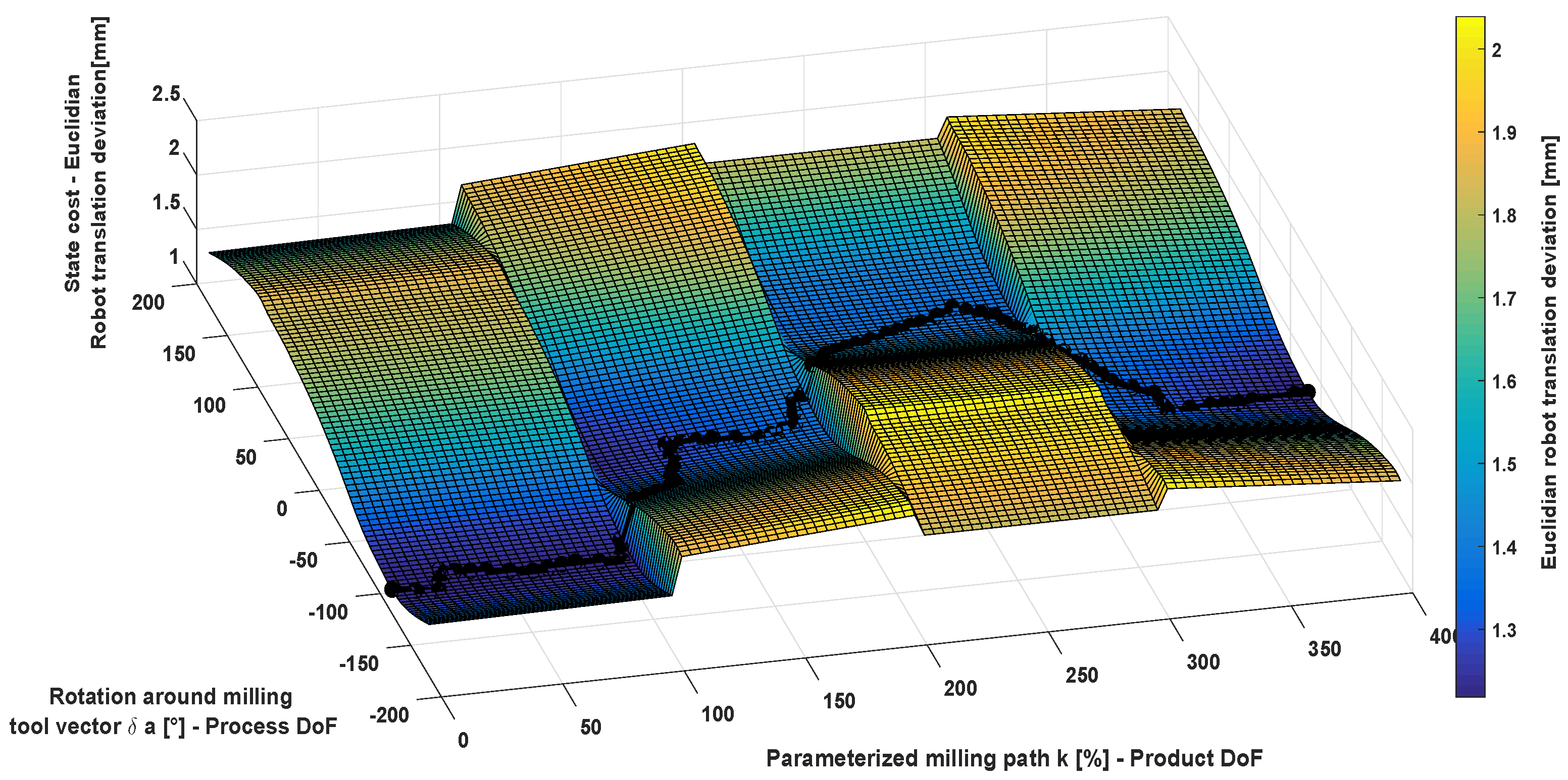
This research contributes with a methodology for interpreting a milling process into a motion problem in which the robot redundancy due to the degree of freedom of the rotation around the milling tool is used for computing an optimal path, using state of the art sample-based motion planning algorithms. The product has been further modeled from its STL file for transforming its constraints into a degree of freedom, which is used in the motion planning phase. Moreover, a semantic description of the milling parameters has been introduced in order to determine the degrees of freedom of the process. Furthermore, the state cost for optimizing stiffness is defined by having as inputs the product and process models and by using the compliance, wrench mapping and the forward and inverse kinematic robot models. The introduction of a simplified space has been also proposed for improving computing performance while using probabilistic planning methods. The automatic procedure for configuring a T-RRT motion planner for optimizing robot stiffness for the milling process has been also introduced.

The presented methodology for the automatic and optimal motion planning problem for the robotic milling motion problem optimizing stiffness has been successfully implemented using state of the art motion planning libraries and tested in simulation. The simulation demonstrates that with the use of the state of the art sample-based motion planning algorithm, transition-based RRT planner, the mechanical work motion cost and the proposed automatic interpretation of the milling process is suitable for being used in CAM environments for optimizing industrial robot motions. Moreover, the approach has demonstrated that the milling process could be methodologically structured and further modeled into the widely-used product, process and resource model, which still has not been used for the planning of robot motions in manufacturing processes. The methodology contributes to the intuitiveness of robot programming and the configurability of robot systems.

Further work requires an exact calibration of robot systems or the compensation using real-time external measuring systems to be able to evaluate in real scenarios the improvements in real machining of the stiffness optimized motion planning. If robot-dependent errors are present, the change in orientations results in undesired deviations, which have not been addressed in this research. Moreover, the methodology and concept could be used in CAM systems integrating validity check functions for approaching, for instance, automatic collision or singularity avoidance. The approach could be also extended to any other machining or manufacturing processes, such as deburring or laser cutting.

References

1. IFR Statistical Department. World Robotics 2014 Industrial Robots; VDMA Robotics + Automation: Frankfurt, Germany, 2014. [Google Scholar]
2. Minhas, S.U.H.; Lehmann, C.; Städter, J.P.; Berger, U. Reconfigurable Strategies for Manufacturing Setups to confront Mass Customization Challenges. In Proceedings of the 21st International Conference on Production Research, Wurttemberg, Germany, 31 July–4 August 2011.
3. Karim, A.; Verl, A. Challenges and obstacles in robot-machining ISR 2013. In Proceedings of the 44th Internationel Symposium on Robotics (IEEE ISR 2013), Seoul, Korea, 24–26 October 2013; pp. 1–4.
4. Slavkovic, N.; Milutinovic, D.; Glavonjic, M. A method for off-line compensation of cutting force-induced errors in robotic machining by tool path modification. Int. J. Adv. Manuf. Technol. 2014, 70, 2083–2096. [Google Scholar] [CrossRef]
5. Iglesias, I.; Sebastián, M.A.; Ares, J.E. Overview of the State of Robotic Machining: Current Situation and Future Potential. Proced. Eng. 2015, 132, 911–917. [Google Scholar] [CrossRef]
6. Schneider, U.; Diaz Posada, J.R.; Drust, M.; Verl, A. Position control of an industrial robot using an optical measurement system for machining purposes. In Advanced Manufacturing Technology XXVII, Proceedings of the 11th International Conference on Manufacturing Research 2013, Incorporating the 28th National Conference on Manufacturing Research 2013, Cranfield, UK, 19 September 2013; pp. 307–312.
7. Schneider, U.; Drust, M.; Ansaloni, M.; Lehmann, C.; Pelliciari, M.; Leali, F.; Gunnink, J.W.; Verl, A. Improving robotic machining accuracy through experimental error investigation and modular compensation. Int. J. Adv. Manuf. Technol. 2016, 85, 3–15. [Google Scholar] [CrossRef] [Green Version]
8. Diaz Posada, J.R.; Schneider, U.; Pidan, S.; Geravand, M.; Stelzer, P.; Verl, A. High accurate robotic drilling with external sensor and compliance model-based compensation. In Proceedings of the 2016 IEEE International Conference on Robotics and Automation (ICRA), Stockholm, Sweden, 16–21 May 2016; pp. 3901–3907.
9. Schneider, U.; Diaz Posada, J.R.; Verl, A. Automatic pose optimization for robotic processes. In Proceedings of the 2015 IEEE International Conference on Robotics and Automation (ICRA), Seattle, WA, USA, 26–30 May 2015; pp. 2054–2059.
10. Lehmann, C.; Halbauer, M.; Euhus, D.; Overbeck, D. Milling with industrial robots: Strategies to reduce and compensate process force induced accuracy influences. In Proceedings of the 17th IEEE International Conference on Emerging Technologies & Factory Automation (ETFA 2012), Krakow, Poland, 17–21 September 2012; Volume 2, pp. 1075–1078.
11. Tyapin, I.; Kaldestad, K.B.; Hovland, G. Off-line path correction of robotic face milling using static tool force and robot stiffness. In Proceedings of the 2015 IEEE/RSJ International Conference on Intelligent Robots and Systems (IROS), Hamburg, Germany, 28 September–2 October 2015; pp. 5506–5511.
12. Abele, E.; Von Stryk, O.; Friedmann, M.; Hemker, T. Prediction of the tool displacement for robot milling applications using coupled models of an industrial robot and removal simulation. In Proceedings of the CIRP 2nd International Conference Process Machine Interactions, Vancouver, BC, Canada, 10–11 June 2010.
13. Abele, E.; Bauer, J.; Rothenbücher, S.; Stelzer, M.; Von Stryk, O. Prediction of the Tool Displacement by Coupled Models of the Compliant Industrial Robot and the Milling Process. In Proceedings of the International Conference on Process Machine Interactions, Hannover, Germany, 3–4 September 2008.
14. Bauer, J. Methoden der Offline-Bahnkorrektur für die spanende Bearbeitung mit Industrierobotern; Schriftenreihe des PTW: Innovation Fertigungstechnik; Epubli-Verlag: Berlin, Germany, 2011. [Google Scholar]
15. Haage, M.; Halbauer, M.; Lehmann, C.; Staedter, J.P. Increasing Robotic Machining Accuracy Using Offline Compensation Based on Joint-Motion Simulation. In Proceedings of the 41st International Symposium on Robotics (ISR/Robotik 2014), Munich, Germany, 24 June 2014; pp. 1–8.
16. Dumas, C.; Caro, S.; Cherif, M.; Garnier, S.; Furet, B. A methodology for joint stiffness identification of serial robots. In Proceedings of the 2010 IEEE/RSJ International Conference on Intelligent Robots and Systems (IROS), Taipei, Taiwan, 18–22 October 2010; pp. 464–469.
17. Klimchik, A.; Wu, Y.; Dumas, C.; Caro, S.; Furet, B.; Pashkevich, A. Identification of geometrical and elastostatic parameters of heavy industrial robots. In Proceedings of the 2013 IEEE International Conference on Robotics and Automation (ICRA), Karlsruhe, Germany, 6–10 May 2013.
18. Abele, E.; Weigold, M.; Rothenbücher, S. Modeling and Identification of an Industrial Robot for Machining Applications. CIRP Ann. Manuf. Technol. 2007, 56, 387–390. [Google Scholar] [CrossRef]
19. Pan, Z.; Zhang, H. Robotic Machining from Programming to Process Control. In Proceedings of the 2008 7th World Congress on Intelligent Control and Automation (WCICA 2008), Chongqing, China, 25–27 June 2008; pp. 553–558.
20. Pan, Z.; Zhang, H. Robotic machining from programming to process control: A complete solution by force control. Ind. Robot 2008, 35, 400–409. [Google Scholar] [CrossRef]
21. Wang, J.; Zhang, H.; Fuhlbrigge, T. Improving machining accuracy with robot deformation compensation. In Proceedings of the 2009 IEEE/RSJ International Conference on Intelligent Robots and Systems, St. Louis, MO, USA, 10–15 October 2009; pp. 3826–3831.
22. Liu, Y.; Cheng, T.; Zuo, L. Adaptive Control Constraint of Machining Processes. Int. J. Adv. Manuf. Technol. 2001, 17, 720–726. [Google Scholar] [CrossRef]
23. Sörnmo, O.; Olofsson, B.; Schneider, U.; Robertsson, A.; Johansson, R. Increasing the Milling Accuracy for Industrial Robots Using a Piezo-Actuated High-Dynamic Micro Manipulator. In Proceedings of the 2012 IEEE/ASME International Conference on Advanced Intelligent Mechatronics (AIM), Kaohsiung, Taiwan, 11–14 July 2012; pp. 104–110.
24. Schneider, U.; Momeni-K, M.; Ansaloni, M.; Verl, A. Stiffness modeling of industrial robots for deformation compensation in machining. In Proceedings of the 2014 IEEE/RSJ International Conference on Intelligent Robots and Systems, Chicago, IL, USA, 14–18 September 2014; pp. 4464–4469.
25. Schneider, U.; Ansaloni, M.; Drust, M.; Leali, F.; Verl, A. Experimental Investigation of Sources of Error in Robot Machining. In Proceedings of International Workshop, WRSM 2013, Porto, Portugal, 26–28 June 2013; pp. 14–26.
26. Dumas, C. Development of Methods for Metal and Composite Parts Trimming with a Robot. Ph.D. Thesis, Université de Nantes, Nantes, France, 2011. [Google Scholar]
27. Schneider, U.; Diaz Posada, J.R.; Drust, M.; Verl, A.; van der Zwaag, J. Combining holistic programming with kinematic parameter optimization for robot machining. In Proceeding of the 41st International Symposium on Robotics (ISR/Robotik 2014), 2–3 June 2014; pp. 524–530.
28. Matsuoka, S.; Shimizu, K.; Yamazaki, N.; Oki, Y. High-speed end milling of an articulated robot and its characteristics. J. Mater. Process. Technol. 1999, 95, 83–89. [Google Scholar] [CrossRef]
29. Budak, E.; Tekeli, A. Maximizing Chatter Free Material Removal Rate in Milling through Optimal Selection of Axial and Radial Depth of Cut Pairs. CIRP Ann. Manuf. Technol. 2005, 54, 353–356. [Google Scholar] [CrossRef]
30. Elbanhawi, M.; Simic, M. Sampling-Based Robot Motion Planning: A Review. IEEE Access 2014, 2, 56–77. [Google Scholar] [CrossRef]
31. LaValle, S.M. Motion Planning: The Essentials. IEEE Robot. Autom. Soc. Mag. 2011, 18, 79–89. [Google Scholar] [CrossRef]
32. Karaman, S.; Frazzoli, E. Sampling-based Algorithms for Optimal Motion Planning. Int. J. Rob. Res. 2011, 30, 846–894. [Google Scholar] [CrossRef]
33. Tsianos, K.I.; Şucan, I.A.; Kavraki, L.E. Sampling-Based Robot Motion Planning: Towards Realistic Applications. Comput. Sci. Rev. 2007, 1, 2–11. [Google Scholar] [CrossRef]
34. Ioan, A.Ş.; Mark, M.; Lydia, E.K. The Open Motion Planning Library. IEEE Robot. Autom. Mag. 2012, 19, 72–82. [Google Scholar]
35. Diaz Posada, J.R.; Dietz, T.; Ockert, P.; Kuss, A.; Hägele, M.; Verl, A. Automatic Optimal Motion Generation for Robotic Manufacturing Processes: Optimal Collision Avoidance in Robotic Welding. In Proceedings of the 2016 12th Conference on Automation Science and Engineering (CASE), Fort Worth, TX, USA, 21–24 August 2016; pp. 154–161.
36. Diaz Posada, J.R.; Kumar, S.; Kuss, A.; Schneider, U.; Drust, M.; Dietz, T.; Verl, A. Automatic Programming and Control for Robotic Deburring. In Proceedings of the ISR 2016: 47st International Symposium on Robotics, Munich, Germany, 21–22 June 2016; pp. 1–8.
37. Kuss, A.; Drust, M.; Verl, A. Detection of workpiece shape deviations for tool path adaptation in robotic deburring systems. In Proceedings of the 49th CIRP CMS Conference on Manufacturing Systems: Factories of the Future in the Digital Environment, Stuttgart, Germany, 25–27 May 2016.
38. Sang, S.C.; Tae, H.Y.; Sang, D.N. XML-based neutral file and PLM integrator for PPR information exchange between heterogeneous PLM systems. Int. J. Comput. Integr. Manuf. 2010, 23, 216–228. [Google Scholar]
39. Drath, R.; Lüder, A.; Peschke, J.; Hundt, L. AutomationML—The glue for seamless automation engineering. In Proceedings of the International Conference on Emerging Technologies and Factory Automation (ETFA), Hamburg, Germany, 15–18 September 2008; pp. 616–623.
40. Gomeringer, R. Tabellenbuch Metall, 46., neu bearb. und erweitere Auflage; Verlag Europa Lehrmittel: Haan-Gruiten, Germany, 2014. [Google Scholar]
41. Jaillet, L.; Cortés, J.; Siméon, T. Sampling-based path planning on configuration-space costmaps. IEEE J. Robot. Autom. 2016, 26, 635–646. [Google Scholar] [CrossRef] [Green Version]
42. Jaillet, L.; Cortés, J.; Siméon, T. Transition-based RRT for path planning in continuous cost spaces. In Proceedings of the International Conference on Intelligent Robots and Systems (IROS), Nice, France, 22–26 September 2008; pp. 2145–2150.
Figure 1. Architecture for the automatic offline motion generation optimizing stiffness for robotic milling (DoF: Degrees of Freedom).
Machines 05 00003 g001
Figure 2. Spaces for the optimal motion generation in robotic milling.
Machines 05 00003 g002
Figure 3. (a) Robot end-effector with the milling tool; (b) robot end-effector with the sensor.
Machines 05 00003 g003
Figure 4. (a) Real and (b) simulated robot machining system.
Machines 05 00003 g004
Figure 5. Illustration of the milling paths on the product and process model and its notations for two edges.
Machines 05 00003 g005
Figure 6. Joint compliance models and their nonlinear descriptions around the z-axes of all six joints.
Machines 05 00003 g006
Figure 7. State cost computation.
Machines 05 00003 g007
Figure 8. Workpiece model and task definition with corners A, B, C and D. Red and green vectors represent the x and y direction of the product frame as described in Section 4.1.
Machines 05 00003 g008
Figure 9. Sequence of robot movements for a four-edge machining task without optimization following the product convention.
Machines 05 00003 g009
Figure 10. State cost elevation map illustration of the motion planning problem for optimizing stiffness.
Machines 05 00003 g010
Figure 11. RMP C-space for the four paths with its state cost (Euclidean robot translation deviations) and a computed optimal path using the T-RRT algorithm.
Machines 05 00003 g011
Figure 12. Sequence of robot movements for a four-edge machining task with stiffness optimization after planning with the T-RRT algorithm.
Machines 05 00003 g012
Figure 13. RMP C-space for the four paths with its state cost (Euclidean robot translation deviations) and a computed optimal path using the T-RRT algorithm.
Machines 05 00003 g013
Figure 14. Translation deviations on x, y, z for the found solution.
Machines 05 00003 g014
Figure 15. (a) Machined workpiece with automatic generated program from the planner with corners A, B, C and D; (b) machined workpiece without optimization following the product convention.
Machines 05 00003 g015
Figure 16. (a) Measured workpiece with automatic generated program from the planner with corners A, B, C and D; (b) measured workpiece without optimization following the product convention.
Machines 05 00003 g016
Figure 17. Depth deviations for compensated and uncompensated mill.
Machines 05 00003 g017