Virtual Reference Feedback Tuning of Model-Free Control Algorithms for Servo Systems


1
Department of Automation and Applied Informatics, Politehnica University of Timisoara, Bd. V. Parvan 2, 300223 Timisoara, Romania
2
School of Electrical Engineering and Computer Science, University of Ottawa, 800 King Edward, Ottawa, ON K1N 6N5, Canada
*
Author to whom correspondence should be addressed.
Machines 2017, 5(4), 25; https://doi.org/10.3390/machines5040025
Submission received: 30 September 2017
/
Revised: 20 October 2017
/
Accepted: 22 October 2017
/
Published: 24 October 2017
Abstract
:This paper proposes the combination of two data-driven techniques, namely virtual reference feedback tuning (VRFT) and model-Free Control (MFC) in terms of the VRFT of MFC algorithms dedicated to servo systems. VRFT ensures the automatic optimal computation of the parameters of three MFC algorithms represented by intelligent proportional (iP), intelligent proportional-integral (iPI), and intelligent proportional-integral-derivative (iPID) controllers. The combination of MFC and VRFT leads to a novel mixed MFC-VRFT approach. The approach is validated by experimental results related to the angular speed control of modular servo system laboratory equipment. The performance of the control systems with the MFC algorithms (iP, iPI, and iPID controllers) tuned by the mixed MFC-VRFT approach is compared with that of control systems with MFC algorithms tuned by a metaheuristics gravitational search algorithm (GSA) optimizer, and of control systems with I, PI and PID controllers optimally tuned by VRFT and GSA in the same optimization problem.
1. Introduction
The feature of data-driven model-free control (MFC) [1] is that it uses only the input/output (I/O) data in order to control unknown processes. MFC is also known in the literature as model-free tuning, as it approximates the process model with a so called ultra-local model, and a rapidly adaptable estimator is used in the process approximation. The control system (CS) stability is guaranteed in MFC if certain constraints are fulfilled. The control algorithms specific to MFC, i.e., the MFC algorithms, are usually referred to as intelligent controllers and the most popular ones are built around proportional (P), proportional-integral (PI), or proportional-integral-derivative (PID) controllers, and are called intelligent proportional (iP), intelligent PI (iPI), and intelligent PID (iPID) controllers. The MFC algorithms have been successfully applied to various processes, such as thermal processes [2], glycemia of type-1 diabetes [3], oscillation damping [4], wheeled autonomous vehicles [5], microalgae cultivation [6], experimental greenhouses [7], surface mounted permanent magnet synchronous motor drive systems [8], and twin rotor aerodynamic systems (TRASs) [9,10]. Recent applications of MFC are reported in [11,12,13]. Other model-free tuning techniques similar to MFC are active disturbance rejection control [14,15,16] and model-free adaptive control (MFAC) [17,18,19].
Virtual reference feedback tuning (VRFT) [20] is another data-driven technique that uses the I/O-collected data of the initial open-loop process, and automatically computes the parameters of linear or nonlinear controllers. The main disadvantage of VRFT is that it does not directly guarantee the closed-loop CS stability. The control algorithms specific to VRFT, i.e., the VRFT algorithms, have been applied recently to TRASs [9,10], two-tank systems [21], quadrotors [22], unmanned gyroplanes [23], non-minimum phase systems [24], robotics [25], and power systems [26].
VRFT has been combined with other data-driven techniques, such as MFC [11], iterative feedback tuning [27], MFAC [28], and reinforcement Q-learning [29]. According to [11] both MFC and VRFT complement each other through their features and they can exhibit improved CS performance by merging them in the so-called mixed MFC-VRFT approach [11].
One major shortcoming of MFC algorithms is that in all previously reported applications the parameters have been chosen empirically and not automatically. The problem is challenging if no process model is available, and it is mitigated here by using VRFT to compute MFC algorithms’ parameters.
Building upon the previous discrete-time implementations of MFC reported in [1,2,3,4,5,6,7,8,9,10,11,12,13] and the mixed MFC-VRFT approach applied to TRASs in [10], this paper proposes a thorough experimental investigation of the new approach, spanning several MFC structures and comparisons with other model-based and model-free tuned controller structures. The main advantages of the proposed approach with respect to the state-of-the-art are:
- -
- It is a widely applicable one-shot data-driven tuning technique that ensures the experiment-based optimal tuning of MFC algorithms.
- -
- -
- It can be easily generalized to other model-free control techniques.
This paper applies the MFC-VRFT approach to a nonlinear modular servo system (MSS) laboratory equipment and compares the performance of CSs with MFC algorithms (iP, iPI, and iPID controllers) tuned by the mixed MFC-VRFT approach with that of control CSs with MFC algorithms tuned by a metaheuristics gravitational search algorithm (GSA) optimizer, of CSs with I, PI, and PID controllers optimally tuned by VRFT, and CSs with I, PI, and PID controllers tuned by GSA.
The main contributions of this paper with the current literature in the field [1,2,3,4,5,6,7,8,9,10,11,12,13] are:
- -
- The mixed MFC-VRFT approach is applied here to an MSS and is experimentally validated by real-time results.
- -
- Three different MFC structures are tuned in this paper using the new approach in order to investigate how the controller structure complexity influences the CS performance.
- -
- The VRFT-based iP, iPI, and iPID controllers are compared against three other model-based and model-free tuned controllers to support the further use of the new model-free tuning approach.
The fair controller comparison is ensured by using the same optimization problem to optimally tune the parameters of both MFC algorithms and linear controllers. Three experimental case studies have been considered, (1), (2), and (3):
- (1)
- The performance of a CS with an iP controller optimally tuned by VRFT is compared with that of a CS with a model-based optimally tuned iP controller. Then the performance of the CSs with iP controllers is compared with that of a CS with an I controller, which is optimally tuned both in a model-based setting and using VRFT (i.e., in a data-driven model-free setting).
- (2)
- The same comparisons and controller tunings are carried out as in the experimental case study (1) but two iPI controllers and two PI controllers are involved.
- (3)
- The experimental case study (1) is applied, but two iPID controllers and two PID controllers are involved.
2. MFC, VRFT, and Mixed MFC-VRFT Approaches
2.1. Overview of MFC
The discrete-time first-order ultra-local model of the unknown single input-single output process is [1]:
where is the controlled output in the case of iP, iPI, and iPID controllers, respectively, with the notation ; is the control signal, ; are the results through the I/O-estimated values and account for the unmodeled dynamics and unknown disturbances, with the notation ; is the discrete time argument; and is a constant chosen by the CS designer such that and have the same order of magnitude.
The control laws specific to iP, iPI, and iPID controllers are [1]:
where are the estimates of , and is the reference input to the feedback CS regarded as a desired trajectory to be tracked. By abuse of notation, are called the P, integral (I), and derivative (D) gains of the iP, iPI, and iPID controllers as they are easily computable in terms of their classical counterparts that appear in the recurrent equations in the error term , such as those in the right-hand side of Equation (2). indicates the tracking error, and, by case, the subscripts iP, iPI, and iPID will be added to and :
is computed from the I/O data and Equation (1) using:
where the subscripts can be iP, iPI, and iPID can be added to , , and depending on the MFC algorithm. A noise-corrupted can compromise the precision of the estimate . Adding a lowpass filter on the measured output will remedy this problem and will also extend the process I/O dynamics, whose bandwidth will decrease. The extended process dynamics are not an issue since unmodeled dynamics are accounted for within the estimated uncertainty . Subsequently, the closed-loop bandwidth will decrease and the CS performance requirements from to have to be re-matched with the dynamics of the extended process.
The difference between and is expressed as:
where is considered a negligible random disturbance in the controller design and tuning [9,10], .
Substituting the iP, iPI, and iPID control laws given in Equation (2) in the model of Equation (1) leads to the dynamics equations of the closed-loop CSs with iP, iPI, and iPID controllers:
The CS structure with MFC algorithms, namely iP, iPI, and iPID controllers, is illustrated in Figure 1.
The substitution of defined in Equation (5) into Equation (6) and in Equation (3) results in the dynamics equation of the tracking error for the CSs with iP, iPI, and iPID controllers:
2.2. Overview on Nonlinear VRFT
The goal of VRFT is to automatically tune the parameters of a linear or nonlinear controller such that the closed-loop CS tracks a reference model [30,31]. With this respect, only the I/O data collected after an open-loop experiment is used as follows: first, a rich frequency spectrum signal must be applied as input on the open-loop process; second, the designer must determine a linear or nonlinear reference model that should specify the behavior of the closed-loop CS.
The performance index used in VRFT is the model reference objective function [31]:
where is the number of samples, is the output of the nonlinear process modeled by the recurrent equation:
where is an unknown nonlinear function, and are the unknown orders of the fixed process structure, is the nonlinear controller output, the nonlinear form of the controller output is is the nonlinear controller parameterized by vector , and the detailed form of the nonlinear controller used in VRFT is:
with and are the known orders of the nonlinear controller parameterized by the vector .
The control (or feedback) error of the closed-loop CS is:
where is the reference input applied to the closed-loop CS. The output of the nonlinear reference model is:
where the reference model is assumed to be invertible and the orders of output and reference input are and .
The unknown linear/nonlinear process is assumed to be I/O stable. The virtual reference input is and it is computed assuming that the output trajectories of the closed-loop CS and the reference model are similar. The virtual control error is next calculated as
According to [31], if is filtered through a richly-parameterized nonlinear controller with parameter vector , the resulting signal should be similar to the open-loop control signal . The controller parameter is determined in terms of minimizing the objective function:
Unlike in the classical linear [20] and nonlinear [30] VRFT where and can be made approximately equal in the vicinity of their minimizing arguments with the use of a prefilter, [31] suggests that, without using the prefilter, and can be minimized by the same argument in the case of a richly parameterized controller.
The design approach of the VRFT structure consists of the following steps:
Step 1.1. Set the initial rich spectrum frequency signal that must be applied as input on the open-loop process and then collect the I/O data after an open-loop experiment.
Step 1.2. Set a linear or nonlinear reference model that should specify the behavior of the closed-loop CS and leads to the virtual reference vector , such that the output trajectories of the closed-loop CS and the reference model are similar.
Step 1.3. Determine the parameter vector by minimizing the objective function in (13).
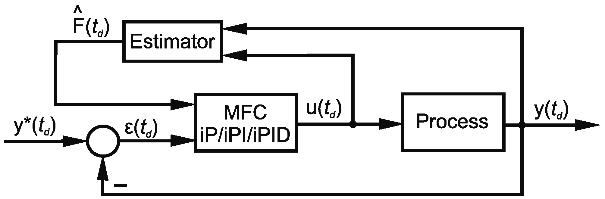
The CS structure controlled with VRFT is presented in Figure 2.
2.3. Mixed MFC-VRFT Approach
This sub-section presents how the VRFT approach is used to automatically compute the parameters of the MFC iP, iPI, and iPID controllers. Unlike [10], where VRFT solely tunes an iP controller, here VRFT also tunes the iPI and iPID controllers, to investigate the increased controller structure complexity over the CS performance.
The equation specific to the MFC law using Equation (4) is:
where is the notation of the block of the MFC law that processes past samples of the feedback error (in similar fashion to P, PI, or PID controllers), and its detailed form is:
where are introduced in Equation (2). Substituting the estimate of in , the detailed control law becomes:
Adding and subtracting the output value and the one step behind sample of the desired trajectory in Equation (16) and then using Equations (3) and (15), the expressions of the control laws specific to the iP, iPI, and iPID controllers are:
The control laws given in Equation (17) are also expressed in the nonlinear forms:
where is linear affine function of its arguments, being parameterized by , , and regarded as tunable vector parameters (with indicating matrix transposition) and are regarded as the non-tunable but known vector parameters and can be treated as either time-varying parameters or exogenous disturbances. The linear affine form of is a particular case of a nonlinear controller structure with integral character. It fits the form of Equation (10), motivating the VRFT.
The VRFT of MFC algorithms is carried out by the mixed MFC-VRFT approach, and the merge of MFC and VRFT is briefly described as follows. The reference input specific to MFC and the virtual reference input specific to VRFT are assumed to be equivalent. The virtual error specific to VRFT and the tracking error specific to MFC are assumed to be equivalent using the fact that is a part of the nonlinear controller equation given in Equation (10), where, depending by the scenario, the parameter vector with the general notation , , can be expressed as , or . The detailed forms of the objective function (13) using these expressions of are:
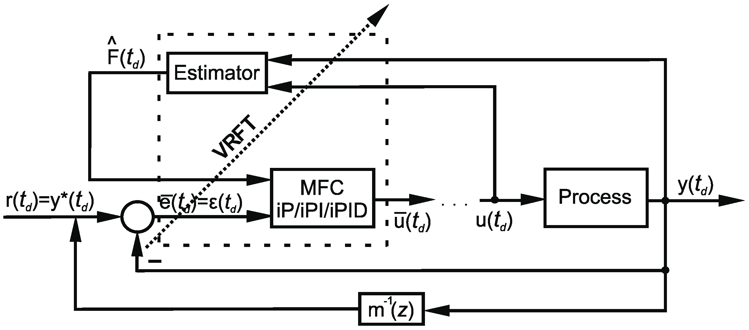
The CS structure with mixed MFC-VRFT algorithms is presented in Figure 3. The MFC algorithms tuned by VRFT in terms of minimizing the first, second and third objective functions in Equation (19) are referred to as VRFT-iP, VRFT-iPI, and VRFT-iPID controllers, respectively.
In summary, the designer must select a linear or nonlinear reference model that specifies the behavior of the closed-loop CS. The I/O data are next collected from the process in a dedicated open-loop experiment. An iP, iPI, or iPID controller structure is selected and the parameter is chosen by the user, then the other tunable parameters are automatically determined by the GSA-based minimization of the objective function in Equation (13). The obtained parameters are used in the closed-loop CSs to track the reference model.
The design approach of the MFC-VRFT structure consists of the following steps:
Step 2.1. Set the design parameter such that and have the same order of magnitude.
Step 2.2. Set the initial rich spectrum frequency signal that must be applied as input on the open-loop process and then collect the I/O data after an open-loop experiment.
Step 2.3. Set a linear or nonlinear reference model that should specify the behavior of the closed-loop CS and leads to the virtual reference vector , such that the output trajectories of the closed-loop CS and the reference model are similar.
Step 2.4. Determine the parameter vector by minimizing the objective function in Equation (13).
3. Experimental Results and Discussion
3.1. The Modular Servo System Equipment
The VRFT-iP, VRFT-iPI, and VRFT-iPID controllers tuned by the mixed MFC-VRFT approach presented in Section 2 are validated on single input-single output MSS laboratory equipment in order to control its velocity. The MSS is illustrated in Figure 4.
The state-space model that describes the nonlinear MSS laboratory equipment and the MSS process parameters are given in [32,33]. The equipment is able to collect discrete-time I/O data from the process in real-time. Therefore, the mixed MFC-VRFT approach will be applied to control this nonlinear process.
3.2. Experimental Validation
Three experimental case studies, (1), (2) and (3), have been considered. Each case study consists of four experimental control scenarios where: (1) the performance of the model-free VRFT-iP and VRFT-I controllers is compared with that of model-based tuned iP and I controllers; (2) the performance of the model-free VRFT-iPI and VRFT-PI controllers is compared with that of model-based tuned iPI and PI controllers; and (3) the performance of the model-free VRFT-iPID and VRFT-PID controllers is compared with that of model-based tuned iPID and PID controllers.
In all experimental case studies, the sampling time has been set to , the number of samples to , and the reference input to a combination of sine, step and ramp signals:
the parameter to has been set in step 2.1, and the discrete transfer function of the linear reference model in all experimental case studies has been set to according to steps 1.2 and 2.3 after applying steps 1.1 and 2.2, respectively:
The performance of CSs with controllers tuned by the mixed MFC-VRFT approach is conditioned by both the choice of the reference model [10,28], and the choice of the initial rich spectrum frequency signal that is applied as input to the open-loop process [31].
The optimization problem defined for the sake of fair comparisons of the performance of VRFT-iP, VRFT-iPI, and VRFT-iPID controllers, VRFT-I, VRFT-PI, and VRFT-PID controllers, and I, PI, and PID controllers, is:
where the vector variable (the parameter vector) depends on the selected experimental case study as follows: in experimental case study (1), in experimental case study (2), and in experimental case study (3) applying step 2.4. The reference model tracking error in (22) is defined as where and are the CS output and the output of the reference model specific to VRFT, respectively, when both the CS and are driven by .
The tunable parameters of VRFT-iP, VRFT-iPI, and VRFT-iPID controllers are automatically determined by minimizing the objective function in Equation (13) using GSA, with the GSA parameters and implementations given in [34,35], and the tunable parameters computed using only the I/O data collected from the nonlinear MSS of the initial open-loop experiment. On the other hand, the parameters of the iP, iPI and iPID controllers and those of the I, PI, and PID controllers are determined by solving the optimization problem in (22) in a model-based setting using the nonlinear MSS process. The problem in Equation (22) is solved via GSA, with the objective function evaluated by the simulation of the CS behavior using the reference input illustrated as follows. The parameters of the VRFT-I, VRFT-PI, and VRFT-PID controllers are computed by minimizing the objective function in Equation (13) through a linear least-squares regression. Therefore, the parameters of VRFT-iP, VRFT-iPI, VRFT-iPID, VRFT-I, VRFT-PI, and VRFT-PID controllers are tuned in a model-free VRFT-based setting applying step 1.3.
Experimental case study (1) consists of four experimental scenarios, where the MSS laboratory equipment is controlled using the optimally-tuned parameters of two model-free VRFT-iP and VRFT-I controllers, and two model-based iP and I controllers. The parameter of the VRFT-iP controller is , the parameter of the iP controller is , the parameter of the model-free VRFT-I controller is , and the model-based I controller parameter is .
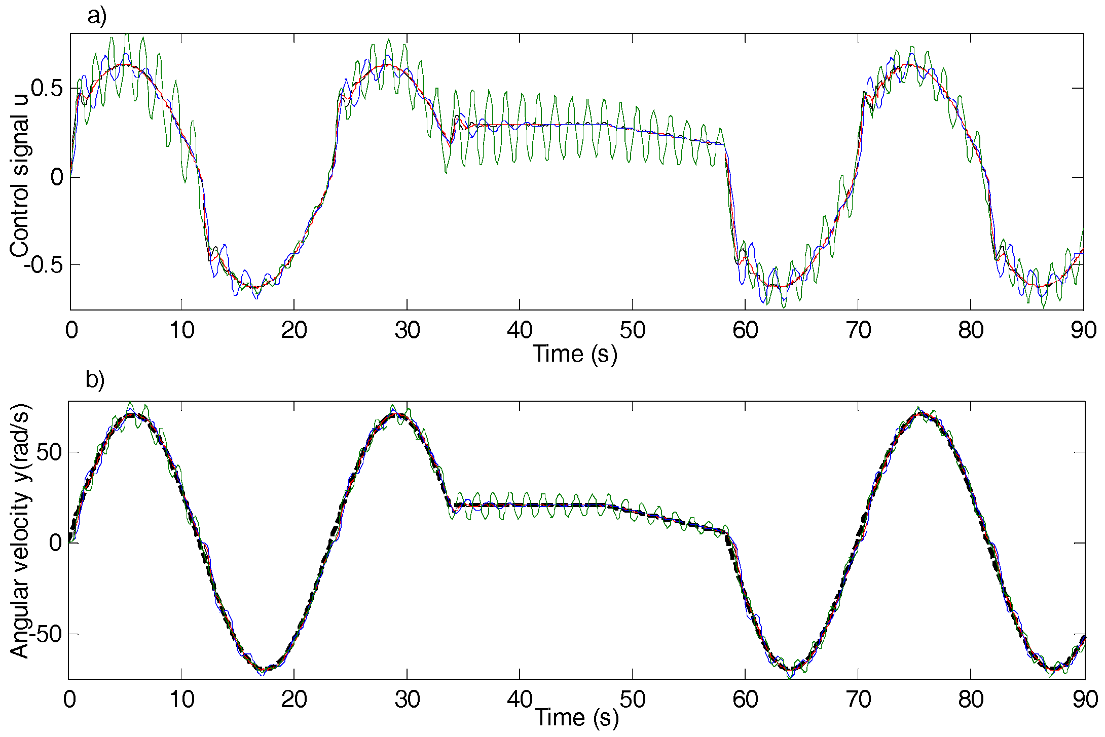
The obtained results have been averaged ten times in order to eliminate the effects of random disturbances. The average and the variance of in the experimental case study (1) are presented in Table 1. Figure 5 illustrates the control signal and the controlled output (the angular velocity) of the CSs with VRFT-iP, iP, VRFT-I and I controllers.
Experimental case study (2) also consists of four experimental scenarios, where the MSS laboratory equipment is controlled using the optimally tuned parameters of VRFT-iPI, iPI, VRFT-PI and PI controllers. The VRFT-iPI controller parameters are , the parameters of the iPI controller are , the parameters of the model-free VRFT-PI controller are , and the parameters of the model-based PI controller are .
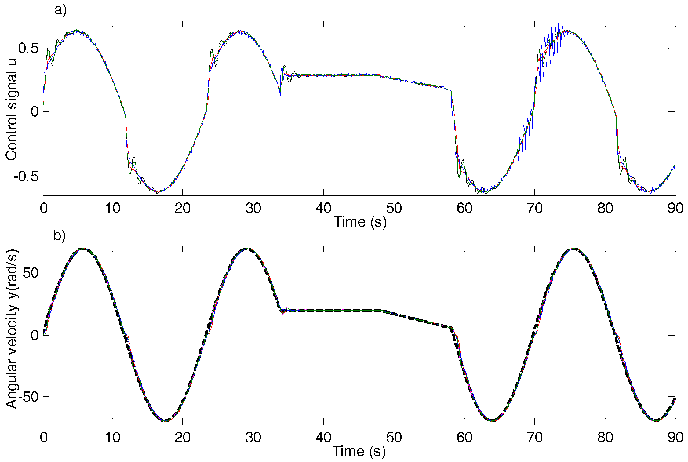
As in the previous case study, the results in the experimental case study (2) have been averaged ten times. Table 2 gives the average and the variance of in experimental case study (2). The control signal and the controlled output of the CSs with VRFT- iPI, iPI, VRFT-PI and PI controllers are presented in Figure 6.
Experimental case study (3) also sums four experimental scenarios, where the MSS laboratory equipment is controlled using the optimally tuned parameters of VRFT- iPID, iPID, and VRFT-PID controllers, and a model-based PID controller. The model-free VRFT-iPID controller parameters are , the iPID controller parameters are , the model-free VRFT-PID controller parameters are obtained as , and the model-based PID controller parameters are obtained as .
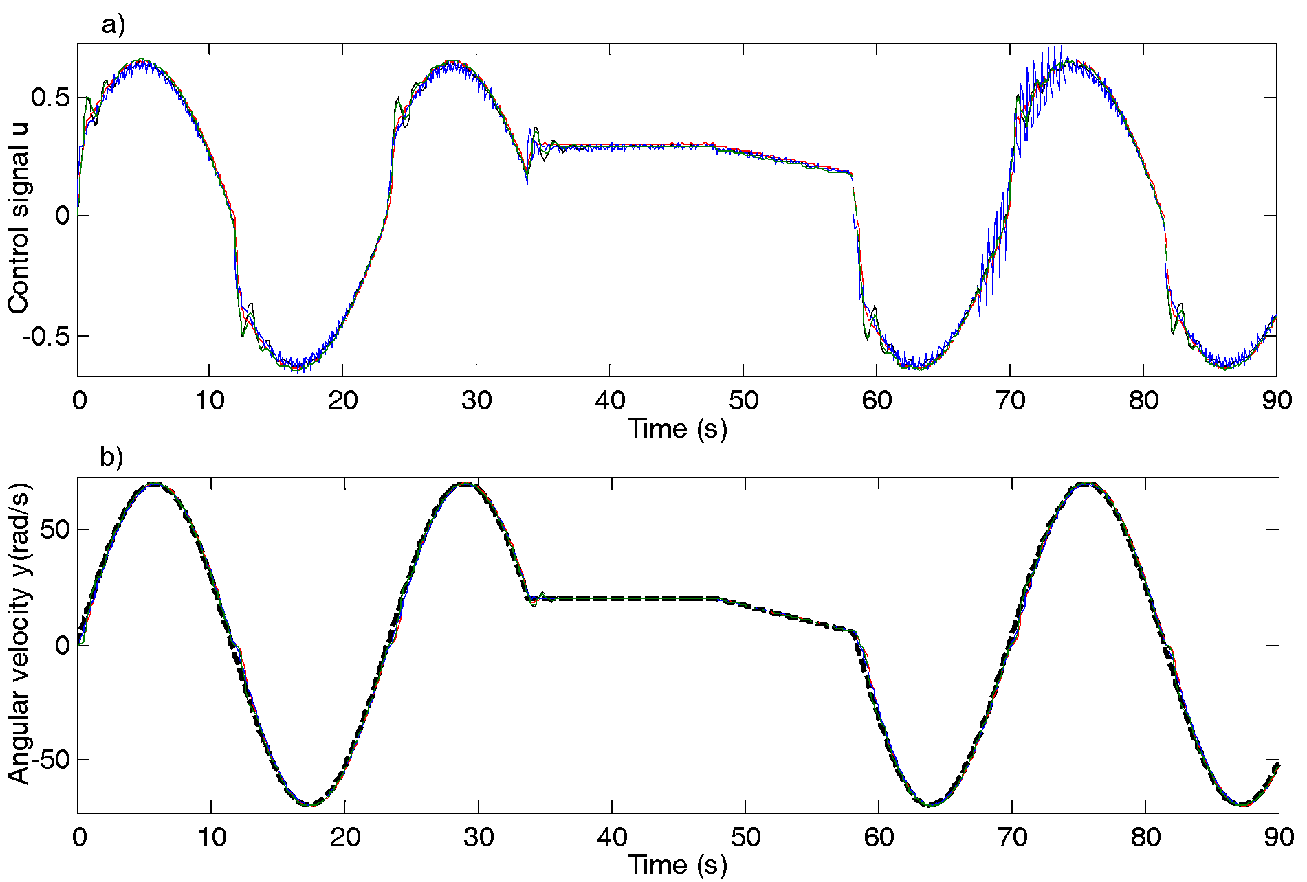
The obtained results given in Table 3 and Figure 7 for experimental case study (3) have also been averaged ten times. The average and the variance of are presented in Table 3. The control signal and the controlled output of the CSs with VRFT-iPID, iPID, VRFT-PID and PID controllers are shown in Figure 7.
The resulted characteristic polynomials of the VRFT-iP, iP, VRFT-iPI, iPI, VRFT-iPID, and iPID controllers together with the roots of the characteristic polynomials resulted from (7) that guarantee the MFC CS stability are presented in Table 4.
3.3. Discussion of Experimental Results
The results obtained in experimental case study (1) show that that the CSs with VRFT-iP and iP controllers exhibit similar performance with the iP controller producing an insignificant advantage. Inserting the controller abbreviations as subscripts in the objective function, Table 1 indicates that . The responses given in Figure 5 illustrate the same, namely, the controlled outputs the CSs with VRFT-iP and iP controllers almost overlap with the reference trajectory signal. Unlike the model-free controllers, the CSs with I controllers tuned via model-free VRFT or GSA exhibit low performance, resulting in some small oscillations at the output, , whereas this controller has a single parameter compared with the iP controller.
The results obtained in experimental case study (2) reveal that VRFT-iPI controller show lower performing than the iPI one, with small differences, namely . This is a somehow normal result, whereas the parameters of the iPI controller have been obtained using the reference trajectory and the mathematical model of the MSS, while the parameters of the VRFT-iPI controller were computed using only the I/O data from the initial open-loop experiment. In this experimental case study, the CS with model-based optimized linear PI controller has better performance than the CS with nonlinear model-free controller, reflected in the objective function ratio, . Unlike the PI controller, the performance of the CS with VRFT-PI controller is somewhere between those of the CSs with VRFT-iPI and iPI controllers as shown in Table 2 and Figure 6. Figure 6 illustrates that all four controlled outputs overlap the reference trajectory.
The results given in Table 3 and Figure 7 for experimental case study (3) outline that the CS with iPID controller tracks better the reference trajectory than the CS with VRFT-iPID controller, i.e., . This is an expected result as the controlled output of the CS with iPID controller overlaps the reference trajectory. The comparison of the best performance of the model-free CSs, namely, the CS with iPID controller, with that of the CS with model-based PID controller, points out that the controlled output of the CS with model-based PID controller exhibits better compared to that of the CS with iPID controller, reflected in . The performance of the CS with VRFT-PID controller is slightly better than that of the CS with VRFT-iPID controller, , but not than that of the CSs with iPID and PID controllers obtained in a model-based setting. Figure 7 illustrates that the differences are almost imperceptible, whereas the controlled outputs almost overlap.
The analysis of the performance of CSs with MFC algorithms tuned by VRFT shows that the best results are obtained for VRFT-iP, followed by VRFT-iPID and VRFT-iPI, and the comparison of the objective function values is .
The comparison of the performance of CSs with MFC algorithms tuned by GSA highlights that the differences between the objective function values for iP, iPI, and iPID controllers are insignificant, as illustrated by . Concluding, the comparison of MFC algorithms tuned by model-free VRFT and model-based GSA proves that no serious improvement is achieved if the intelligent MFC adaptive structure complexity expressed in number of parameters is increased.
The comparison of the performances of CSs with linear I, PI, and PID controllers tuned by VRFT shows that the VRFT-PI and the VRFT-PID controllers perform eight times better than the VRFT-I controller and the objective function comparison is .
The comparison of CSs with linear I, PI and PID controllers tuned in a model-based setting reveals that the I controller has lower performance than the PI and PID ones. The CSs with PI and PID controllers perform ten times better than the CS with I controller, namely, .
The experimental results presented in case studies (1), (2), and (3) indicate that, on one hand, better reference model tracking performance is achieved if the model-based tuning of iP, iPI, and iPID controllers is carried out versus the model-free MFC-VRFT approach, although the differences between model-free VRFT tuning and model-based optimal tuning (using GSA) of MFC algorithms are not high. This is considered normal because using the process model knowledge is expected to give superior performance.
On the other hand, the model-based optimal tuning results show that the classical linear PI and PID controllers outperform the iPI and iPID controllers, respectively, except the I versus the iP controller. In the case of I and iP controllers it is in fact normal that the latter is better as it actually has an integral component in the first expression in Equation (17), although it is only called iP. As such, even if it has only one tunable parameter, the iP controller more accurately resembles a pure integral controller. Thus, the complexity of MFC algorithms is not really justified in the iPI and iPID cases. According to the obtained results, in the model-free case, better performance is achieved using the VRFT-iP controller versus the VRFT-iPI, VRFT-iPID, iPID, VRFT-I, VRFT-PI, and VRFT-PID controllers, although the VRFT-iP controller has only one tunable parameter. As specified in the previous section, the MFC algorithms have an additional parameter, , which, in this case, was not subjected to tuning, but it has been set by the designer, indicating a further shortcoming of MFC algorithms.
Since no major differences exist between model-based and model-free tuning in this application, it is more advantageous to tune the controller parameters using model-free VRFT. Our new mixed MFC-VRFT approach saves time as it automatically tunes the parameters of the MFC algorithms.
Arguably, the VRFT approach translates the selection of MFC parameters into the selection of reference model parameters, which may be considered just a problem reformulation. However, it is always preferable to prescribe performance in terms of the easily-interpretable indices of reference model responses, such as response time and overshoot. Nevertheless, this required performance has to be matched with the process dynamics.
However, the 11 comparisons included will lead to different conclusions if other nonlinear processes as those illustrative given in [36,37,38,39,40,41,42] will be controlled. Several other objective functions can be considered [43,44,45,46,47,48,49].
GSA has been used to solve the optimization problems in this paper because of the inspiration from Newton’s law of gravity and law of motion. This specifically gives the strength of GSA in the exploration that belongs to the search process of optimization algorithms. This also makes the difference and superiority with respect to other metaheuristics optimizers, including particle swarm optimization, simulated annealing, genetic programming, and genetic algorithms, which are advantageous in the exploitation.
4. Conclusions
This paper has proposed a novel mixed MFC-VRFT approach. This approach has been accompanied by the implementation and application of a set of controllers, i.e., VRFT-iP, VRFT-iPI, and VRFT-iPID. These controllers have been compared experimentally with iP, iPI, iPID, VRFT-I, VRFT-PI, VRFT-PID, and model-based optimal I, PI, and PID controllers in order to control the angular velocity of a nonlinear MSS laboratory equipment containing. Three case studies, each one consisting of four experimental scenarios, have been defined for the fair comparison of all controllers.
The discussion of the experimental results highlights that if the MFC-VRFT approach suggested in the paper is applied to similar nonlinear servo systems, it is recommended to use a model-free VRFT-iP controller.
Future research will be dedicated to improving the performance of CSs with MFC algorithms and comparing it with other data-driven techniques, such as model-free adaptive control, active disturbance rejection control, iterative feedback tuning, or reinforcement Q-learning. The analysis of the superiority of model-based tuning if poor process models are used will be treated as well.
Acknowledgments
This work was supported by grants from the partnerships in priority areas—the PN II program of the Romanian Ministry of Research and Innovation—the Executive Agency for Higher Education, Research, Development and Innovation Funding (UEFISCDI), project numbers PN-II-PT-PCCA-2013-4-0544 and PN-II-PT-PCCA-2013-4-0070, by a grant from the Romanian National Authority for Scientific Research (CNCS)–UEFISCDI, project number PN-II-RU-TE-2014-4-0207, and by a grant from NSERC of Canada.
Author Contributions
Raul-Cristian Roman wrote the paper, performed the experiments, and analyzed the algorithms; Mircea-Bogdan Radac prepared the theoretical results in Section 2.3 and automated the experiments; Radu-Emil Precup revised the mathematical formulations and ensured the hardware and software support; Emil M. Petriu revised the paper and ensured the systematic comparison and validation. All authors have read and approved the final paper.
Conflicts of Interest
The authors declare no conflict of interest.
References
- Fliess, M.; Join, C. Model-free control. Int. J. Control 2013, 86, 2228–2252. [Google Scholar] [CrossRef] [Green Version]
- Carrillo, F.J.; Rotella, F. Some contributions to estimation for mode-free control. In Proceedings of the 17th IFAC Symposium on System Identification, Beijing, China, 19–21 October 2015; pp. 150–155. [Google Scholar]
- Ridha, T.M.; Moog, C.H. Model free control for type-1 diabetes: A fasting-phase study. In Proceedings of the 9th IFAC Symposium on Biological and Medical Systems, Berlin, Germany, 31 August–2 September 2015; pp. 76–81. [Google Scholar]
- Jama, M.A.; Noura, H.; Wahyudie, A.; Assi, A. Enhancing the performance of heaving wave energy converters using model-free control approach. Renew. Energy 2015, 83, 931–941. [Google Scholar] [CrossRef]
- D’Andrea-Novel, B.; Menhour, L.; Fliess, M.; Mounier, H. Some remarks on wheeled autonomous vehicles and the evolution of their control design. In Proceedings of the 9th IFAC Symposium on Intelligent Autonomous Vehicles, Leipzig, Germany, 29 June–1 July 2016; pp. 1–6. [Google Scholar]
- Tebbani, S.; Titica, M.; Join, C.; Fliess, M.; Dumur, D. Model-based versus model-free control designs for improving microalgae growth in a closed photobioreactor: Some preliminary comparisons. In Proceedings of the 24th Mediterranean Conference on Control and Automation, Athens, Greece, 21–24 June 2016; pp. 1–6. [Google Scholar]
- Lafont, F.; Balmat, J.-F.; Pessel, N.; Fliess, M. A model-free control strategy for an experimental greenhouse with an application to fault accommodation. Comput. Electron. Agric. 2015, 110, 139–149. [Google Scholar] [CrossRef]
- Zhou, Y.; Li, H.-M.; Yao, H.-Y. Model-free control of surface mounted PMSM drive system. In Proceedings of the 2016 IEEE International Conference on Industrial Technology, Taipei, Taiwan, 14–17 March 2016; pp. 175–180. [Google Scholar]
- Roman, R.-C.; Radac, M.-B.; Precup, R.-E. Multi-input-multi-output system experimental validation of model-free control and virtual reference feedback tuning techniques. IET Control Theory Appl. 2016, 10, 1395–1403. [Google Scholar] [CrossRef]
- Roman, R.-C.; Radac, M.-B.; Precup, R.-E. Mixed MFC-VRFT approach for multivariable aerodynamic system position control. In Proceedings of the 2016 IEEE International Conference on Systems, Man, and Cybernetics, Budapest, Hungary, 9–12 October 2016; pp. 2615–2620. [Google Scholar]
- Wang, H.-P.; Ye, X.-F.; Tian, Y.; Zheng, G.; Christov, N. Model-free-based terminal SMC of quadrotor attitude and position. IEEE Trans. Aerosp. Electron. Syst. 2016, 52, 2519–2528. [Google Scholar] [CrossRef]
- Precup, R.-E.; Radac, M.-B.; Roman, R.-C.; Petriu, E.M. Model-free sliding mode control of nonlinear systems: Algorithms and experiments. Inf. Sci. 2017, 381, 176–192. [Google Scholar] [CrossRef]
- Abouaïssa, H.; Fliess, M.; Join, C. On ramp metering: Towards a better understanding of ALINEA via model-free control. Int. J. Control 2017, 90, 1018–1026. [Google Scholar] [CrossRef] [Green Version]
- Han, J.Q. From PID to active disturbance rejection control. IEEE Trans. Ind. Electron. 2009, 56, 900–906. [Google Scholar] [CrossRef]
- Xia, Y.Q.; Pu, F.; Li, S.F.; Gao, Y. Lateral path tracking control of autonomous land vehicle based on ADRC and differential flatness. IEEE Trans. Ind. Electron. 2016, 63, 3091–3099. [Google Scholar] [CrossRef]
- Herbst, G. Practical active disturbance rejection control: Bumpless transfer, rate limitation, and incremental algorithm. IEEE Trans. Ind. Electron. 2016, 63, 1754–1762. [Google Scholar] [CrossRef]
- Hou, Z.S.; Jin, S. A novel data-driven control approach for a class of discrete-time nonlinear systems. IEEE Trans. Control Syst. Technol. 2011, 19, 1549–1558. [Google Scholar] [CrossRef]
- Hou, Z.S.; Zhu, Y.M. Controller-dynamic-linearization-based model free adaptive control for discrete-time nonlinear systems. IEEE Trans. Ind. Inform. 2013, 9, 2301–2309. [Google Scholar] [CrossRef]
- Pang, Z.-H.; Liu, G.-P.; Zhou, D.H.; Sun, D.H. Data-based predictive control for networked nonlinear systems with network-induced delay and packet dropout. IEEE Trans. Ind. Electron. 2016, 63, 1249–1257. [Google Scholar] [CrossRef]
- Campi, M.C.; Lecchini, A.; Savaresi, S.M. Virtual reference feedback tuning: A direct method for the design of feedback controllers. Automatica 2002, 38, 1337–1346. [Google Scholar] [CrossRef]
- Campestrini, L.; Eckhard, D.; Chía, L.A.; Boeira, E. Unbiased MIMO VRFT with application to process control. J. Proc. Control 2016, 39, 35–49. [Google Scholar] [CrossRef]
- Invernizzi, D.; Panizza, P.; Riccardi, F.; Formentin, S.; Lovera, M. Data-driven attitude control law of a variable-pitch quadrotor: A comparison study. IFAC PapersOnLine 2016, 49, 236–241. [Google Scholar] [CrossRef]
- Wang, Y.; Tang, X.-J. Attitude controller optimization for unmanned gyroplane using online virtual reference feedback control. In Proceedings of the 35th Chinese Control Conference, Chengdu, China, 27–29 July 2016; pp. 10754–10758. [Google Scholar]
- Gonçalves da Silva, G.R.; Campestrini, L.; Bazanella, A.S. Multivariable VRFT: An approach for systems with non-minimum phase transmission zeros. In Proceedings of the 2016 IEEE Conference on Control Applications, Buenos Aires, Argentina, 19–22 September 2016; pp. 1324–1329. [Google Scholar]
- Yamamoto, N.; Yubai, K.; Yashiro, D.; Komada, S. Direct design method of force controller based on input/output data. In Proceedings of the 2016 International Conference on Advanced Mechatronics Systems, Melbourne, Australia, 30 November–3 December 2016; pp. 126–131. [Google Scholar]
- Jeng, J.-C.; Yeh, C.-H. Coordinated control design for a PEMFC power system using adaptive VRFT method. J. Taiwan Inst. Chem. Eng. 2017, 73, 102–111. [Google Scholar] [CrossRef]
- Radac, M.-B.; Grad, R.-B.; Precup, R.-E.; Petriu, E.M.; Preitl, S.; Dragos, C.-A. Mixed virtual reference feedback tuning-iterative feedback tuning: Method and laboratory assessment. In Proceedings of the 2011 IEEE International Symposium on Industrial Electronics, Gdansk, Poland, 27–30 June 2011; pp. 649–654. [Google Scholar]
- Roman, R.-C.; Radac, M.-B.; Precup, R.-E.; Petriu, E.M. Data-driven model-free adaptive control tuned by virtual reference feedback tuning. Acta Polytech. Hung. 2016, 13, 83–96. [Google Scholar]
- Radac, M.-B.; Precup, R.-E.; Roman, R.-C. Model-free control performance improvement using virtual reference feedback tuning and reinforcement Q-learning. Int. J. Syst. Sci. 2017, 48, 1071–1083. [Google Scholar] [CrossRef]
- Campi, M.C.; Savaresi, S.M. Direct nonlinear control design: The Virtual Reference Feedback Tuning (VRFT) approach. IEEE Trans. Autom. Control 2006, 65, 14–27. [Google Scholar] [CrossRef]
- Yan, P.; Liu, D.; Wang, D.; Ma, H. Data-driven controller design for general MIMO nonlinear systems via virtual reference feedback tuning and neural networks. Neurocomputing 2016, 171, 815–825. [Google Scholar] [CrossRef]
- Inteco Ltd. Modular Servo System, User’s Manual; Inteco Ltd.: Krakow, Poland, 2006. [Google Scholar]
- Precup, R.-E.; David, R.-C.; Petriu, E.M. Grey wolf optimizer algorithm-based tuning of fuzzy control systems with reduced parametric sensitivity. IEEE Trans. Ind. Electron. 2017, 64, 527–534. [Google Scholar] [CrossRef]
- Precup, R.-E.; Angelov, P.; Costa, B.S.J.; Sayed-Mouchaweh, M. An overview on fault diagnosis and nature-inspired optimal control of industrial process applications. Comput. Ind. 2015, 74, 75–94. [Google Scholar] [CrossRef]
- Precup, R.-E.; Sabau, M.-C.; Petriu, E.M. Nature-inspired optimal tuning of input membership functions of Takagi-Sugeno-Kang fuzzy models for anti-lock braking systems. Appl. Soft Comput. 2015, 27, 575–589. [Google Scholar] [CrossRef]
- Del Toro, R.M.; Schmittdiel, M.C.; Haber-Guerra, R.-E.; Haber-Haber, R. System identification of the high performance drilling process for network-based control. In Proceedings of the 21st Biennial Conference on Mechanical Vibration and Noise, Las Vegas, NV, USA, 4–7 September 2007; pp. 827–834. [Google Scholar]
- Bošnak, M.; Matko, D.; Blažič, S. Quadrocopter hovering using position-estimation information from inertial sensors and a high-delay video system. J. Intell. Robot. Syst. 2012, 67, 43–60. [Google Scholar] [CrossRef]
- Wijayasekara, D.; Linda, O.; Manic, M.; Rieger, C. FN-DFE: Fuzzy-Neural Data Fusion Engine for enhanced resilient state-awareness of hybrid energy systems. IEEE Trans. Cybern. 2014, 44, 2065–2075. [Google Scholar] [CrossRef] [PubMed]
- Noroozi, N.; Khayatian, A.; Ahmadizadeh, S.; Karimi, H.R. On integral input-to-state stability for a feedback interconnection of parameterised discrete-time systems. Int. J. Syst. Sci. 2016, 47, 1598–1614. [Google Scholar] [CrossRef]
- Gharbi, A.; Benrejeb, M.; Borne, P. A taboo search optimization of the control law of nonlinear systems with bounded uncertainties. Int. J. Comput. Communic. Control 2016, 11, 224–232. [Google Scholar] [CrossRef]
- Yin, S.; Shi, P.; Yang, H.Y. Adaptive fuzzy control of strict-feedback nonlinear time-delay systems with unmodeled dynamics. IEEE Trans. Cybern. 2016, 46, 1926–1938. [Google Scholar] [CrossRef] [PubMed]
- Wang, L.J.; Li, H.Y.; Zhou, Q.; Lu, R.Q. Adaptive fuzzy control for nonstrict feedback systems with unmodeled dynamics and fuzzy dead zone via output feedback. IEEE Trans. Cybern. 2017, 47, 2400–2412. [Google Scholar] [CrossRef] [PubMed]
- Filip, F.G. Decision support and control for large-scale complex systems. Ann. Rev. Control 2008, 32, 61–70. [Google Scholar] [CrossRef]
- Vaščák, J. Adaptation of fuzzy cognitive maps by migration algorithms. Kybernetes 2012, 41, 429–443. [Google Scholar] [CrossRef]
- Maithripala, D.H.S.; Dayawansa, W.P.; Berg, J.M. Intrinsic observer-based stabilization for simple mechanical systems on Lie groups. SIAM J. Control Optim. 2015, 44, 1691–1711. [Google Scholar] [CrossRef]
- Solos, I.P.; Tassopoulos, I.X.; Beligiannis, G.N. Optimizing shift scheduling for tank trucks using an effective stochastic variable neighbourhood approach. Int. J. Artif. Intell. 2016, 14, 1–26. [Google Scholar]
- Ducic, N.; Cojbašic, Ž.; Radiša, R.; Slavkovic, R.; Milicevic, I. CAD/CAM design and genetic optimization of feeders for sand casting process. Facta Univ. Ser. Mech. Eng. 2016, 14, 147–158. [Google Scholar]
- Ali, M.Z.; Awad, N.H.; Duwairi, R.M. Multi-objective differential evolution algorithm with a new improved mutation strategy. Int. J. Artif. Intell. 2016, 14, 23–41. [Google Scholar]
- Cabrera-Guerrero, P.; Moltedo-Perfetti, A.; Cabrera, E.; Paredes, F. Comparing two heuristic local search algorithms for a complex routing problem. Stud. Inform. Control 2016, 25, 411–420. [Google Scholar] [CrossRef]
Figure 1.
The CS structure with iP, iPI, and iPID controllers.

Figure 2.
The CS structure controlled with VRFT.
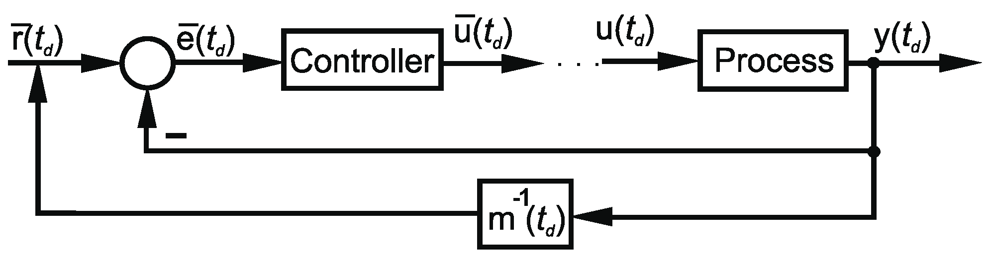
Figure 3.
The CS structure with mixed MFC-VRFT algorithms.

Figure 4.
The MSS.
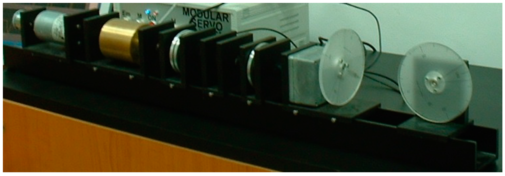
Figure 5.
Experimental results of case study (1): control signal of CS with VRFT-iP (black), CS with iP (red), CS with VRFT-I (green), and CS with I (blue) controllers in (a); reference trajectory (solid black dashed), controlled output of CS with VRFT-iP (black), CS with iP (red), CS with VRFT-I (green), and CS with I (blue) controllers in (b).

Figure 6.
Experimental results of case study (2): control signal of CS with VRFT-iPI (black), CS with iPI (red), CS with VRFT-PI (green), and CS with PI (blue) controllers in (a); reference trajectory (solid black dashed), controlled output of CS with VRFT-iPI (black), CS with iPI (red), CS with VRFT-PI (green), and CS with PI (blue) controllers in (b).

Figure 7.
Experimental results of case study (3): control signal of CS with VRFT-iPID (black), CS with iPID (red), CS with VRFT-PID (green), and CS with PID (blue) controllers in (a); reference trajectory (solid black dashed), controlled output of CS with VRFT-iPID (black), CS with iPID (red), CS with VRFT-PID (green), and CS with PID (blue) controllers in (b).


Table 1.
Objective function values in the experimental case study (1).
| Scenario | Average of | Variance of |
|---|---|---|
| VRFT-iP | 1.8832 | 0.0057 |
| iP | 1.8101 | 0.0042 |
| VRFT-I | 16.5884 | 2.8952 |
| I | 8.0407 | 0.1565 |
Table 2.
Objective function values in experimental case study (2).
| Scenario | Average of | Variance of |
|---|---|---|
| VRFT-iPI | 2.4645 | 0.0151 |
| iPI | 1.5565 | 0.0033 |
| VRFT-PI | 2.0542 | 0.0071 |
| PI | 0.7675 | 0.0007 |
Table 3.
Objective function values in experimental case study (3).
| Scenario | Average of | Variance of |
|---|---|---|
| VRFT-iPID | 2.2834 | 0.0062 |
| iPID | 1.4742 | 0.0102 |
| VRFT-PID | 2.0134 | 0.0107 |
| PID | 0.7636 | 0.0009 |
Table 4.
The characteristic polynomials and the roots resulted from Equation (7).
| Scenario | Characteristic Polynomials | Roots of the Characteristic Polynomials |
|---|---|---|
| VRFT-iP | ||
| iP | ||
| VRFT-iPI | ||
| iPI | ||
| VRFT-iPID | ||
| iPID |
© 2017 by the authors. Licensee MDPI, Basel, Switzerland. This article is an open access article distributed under the terms and conditions of the Creative Commons Attribution (CC BY) license (http://creativecommons.org/licenses/by/4.0/).
Share and Cite
MDPI and ACS Style
Roman, R.-C.; Radac, M.-B.; Precup, R.-E.; Petriu, E.M. Virtual Reference Feedback Tuning of Model-Free Control Algorithms for Servo Systems. Machines 2017, 5, 25. https://doi.org/10.3390/machines5040025
AMA Style
Roman R-C, Radac M-B, Precup R-E, Petriu EM. Virtual Reference Feedback Tuning of Model-Free Control Algorithms for Servo Systems. Machines. 2017; 5(4):25. https://doi.org/10.3390/machines5040025
Chicago/Turabian StyleRoman, Raul-Cristian, Mircea-Bogdan Radac, Radu-Emil Precup, and Emil M. Petriu. 2017. "Virtual Reference Feedback Tuning of Model-Free Control Algorithms for Servo Systems" Machines 5, no. 4: 25. https://doi.org/10.3390/machines5040025
Note that from the first issue of 2016, this journal uses article numbers instead of page numbers. See further details here.