System Identification Algorithm for Computing the Modal Parameters of Linear Mechanical Systems


Department of Industrial Engineering, University of Salerno, Via Giovanni Paolo II 132, 84084 Fisciano, Italy
*
Author to whom correspondence should be addressed.
Machines 2018, 6(2), 12; https://doi.org/10.3390/machines6020012
Submission received: 1 March 2018
/
Revised: 22 March 2018
/
Accepted: 23 March 2018
/
Published: 26 March 2018
(This article belongs to the Special Issue Advanced Control Systems and Optimization Techniques)
Abstract
:The goal of this investigation is to construct a computational procedure for identifying the modal parameters of linear mechanical systems. The methodology employed in the paper is based on the Eigensystem Realization Algorithm implemented in conjunction with the Observer/Kalman Filter Identification method (ERA/OKID). This method represents an effective and efficient system identification numerical procedure based on the time domain. The algorithm developed in this work is tested by means of numerical experiments on a full-car vehicle model. To this end, the modal parameters necessary for the design of active and semi-active suspension systems are obtained for the vehicle system considered as an illustrative example. In order to analyze the performance of the methodology developed in this investigation, the system identification numerical procedure was tested considering two case studies, namely a full state measurement and an incomplete state measurement. As expected, the numerical results found for the identified dynamical model showed a good agreement with the modal parameters of the mechanical system model. Furthermore, numerical results demonstrated that the proposed method has good performance considering a scenario in which the signal-to-noise ratio of the input and output measurements is relatively high. The method developed in this paper can be effectively used for solving important engineering problems such as the design of control systems for road vehicles.
1. Introduction
In abstract terms, a mathematical model of a dynamical system is a specific pattern that establishes relationships between the physical input and output quantities that can also be observed experimentally. A mathematical model of a dynamical system, therefore, allows for predicting the system dynamic behavior in response to a given set of external excitations [1]. The complexity of a dynamical model reflects the model dimension, its general flexibility and the capacity of representing the phenomena of interest in terms of mathematical laws [2,3,4,5]. The complexity of a given dynamical model is strongly correlated with the mathematical structure of the model and to the information content present in the observed dataset used in the model development. In this context, the estimation process is an iterative process in which the mathematical structure of a dynamical model is devised and, once a suitable mathematical model is constructed for capturing the physics of the system of interest, one can identify the unknown parameters in the model by using an experimental dataset [6,7,8,9]. This process is guided by the intuition of the analyst and is based on the useful information embedded in the dataset available from the experimental campaign [10,11,12,13,14,15,16]. In the validation process, on the other hand, the analyst verifies that the selected dynamical model and the identified model parameters are able to reproduce the input-output datasets that are different from those used for constructing the system model by means of the system identification methods. The main advantage of having an analytical model of a mechanical system is represented by the possibility of performing numerical experiments by using dynamic simulations, which are inexpensive, safe and can be repeated for reproducing a large number of different realistic scenarios [17,18,19]. However, the accuracy and reliability of the numerical results computed through dynamic simulations completely depend on the quality of the mathematical model of the physical system identified by using the observed dataset [20,21,22].
This investigation is grounded in the mathematical tools of the scientific discipline called system identification. Originally developed in the field of control theory, system identification has become an independent field of scientific research that is focused on the determination of a mathematical model for a physical system by using experimental data [23,24,25]. In order to achieve this goal, the analyst should combine the information arising from experimental data with the background knowledge on the functioning of a particular dynamical system. The mathematical techniques used in the field of the system identification serve a threefold objective, namely: they can be employed for identifying a set of unknown parameters of a nonlinear mathematical model by using an experimental dataset; they can be used for the determination of the model order corresponding to a given system; and they allow for obtaining finite-dimensional linear models of a general mechanical system starting from an interrelated sequence of input-output data [26,27]. The methods of system identification can be applied to deterministic systems, as well as to stochastic processes [28,29]. Furthermore, several effective system identification methods have been developed in the literature such as, for example, adaptive algorithms, least square methods, gradient-based procedures and multi-innovation identification methodologies [30,31,32,33,34,35]. In engineering applications, the methods of system identification are principally used for performing the experimental modal analysis, which represents the principal topic of interest of this investigation. To this end, two general approaches can be employed, namely the time-domain analysis and the frequency-domain analysis [36]. In the time-domain analysis, the input-output dataset obtained in an experimental campaign is directly provided to the system identification numerical procedures based on the time domain. On the other hand, in the frequency domain analysis, the experimental data are filtered and used by means of a Fourier transform, and subsequently, they are used in a system identification numerical procedure based on the frequency domain. In both cases, the analyst is interested in the calculation of the number of normal modes and natural frequencies necessary for constructing a reliable dynamic model of a given mechanical system without directly deriving the system equations of motion [37,38,39,40].
In mechanical engineering applications, various studies focused on the active and passive control problem of machines and structures based on the mathematical techniques developed in the field of system identification and optimal control can be found [41,42,43,44]. The optimal control problem is particularly challenging in the case of rigid and flexible multibody systems, which represent mechanical systems formed by continuum bodies, kinematic joints, force fields and control actuators [45,46,47,48,49,50]. Another important application of the system identification scientific discipline is the refinement of a finite element model through dynamic testing for the design of vibration control systems based on open-loop and closed-loop control schemes [51,52,53,54]. The methodologies of time domain analysis employed in the general area of applied system identification are of interest for this investigation because the state-space models obtained through these numerical procedures can be readily used for developing effective control actions employing well-established and robust algorithms, such as, for example, the pole placement method, the linear-quadratic regulator technique and the H-infinity method, as well as more advanced nonlinear control approaches [55,56,57,58,59,60,61]. In the case of the parametric identification problem, one needs to construct analytical expressions in terms of the desired parameters and correlate them with experimental data in order to identify the parameters of interest [62,63]. For this purpose, simple least-square methods, as well as more advanced gradient-based optimization techniques relying on the adjoint method can be used for minimizing the error between the time responses observed in experimental measurements and the time evolutions predicted by the mathematical model based on the unknown parameters [64,65,66,67,68,69]. On the other hand, in the case of the model identification problem in the time domain, one needs to find a linear dynamical model directly that embodies the best fit for an input and output dataset measured for a given mechanical system. The model identification problem is based on analytical techniques and numerical linear algebra methods that are of interest for this work and, therefore, are discussed in this paper.
This manuscript is subdivided as follows. In Section 2, the mathematical background related to the system identification numerical procedure developed in this investigation is provided. In Section 3, a full-car mechanical model of a standard road vehicle is analyzed and used as a demonstrative example for the system identification numerical procedure considered in this work. In Section 4, the summary of the paper, the conclusions of these investigations and a discussion about the future directions of research are reported.
2. System Identification Algorithm
This section describes the background material necessary for the analytical development and the computer implementation of the system identification numerical procedure employed in this investigation for obtaining the modal parameters of a mechanical system characterized by a linear mathematical structure.
2.1. Representation of the Dynamical Model in the Space of States
In this subsection, the key aspects of the mathematical description of a mechanical system considering a representation in the space of states are illustrated. For this purpose, the dynamic equations of a mechanical system having a linear mathematical structure are considered. The equations of motion form a coupled set of second-order linear ordinary differential equations, where is the number of the generalized coordinates used in the mathematical model that form an independent set of time-varying parameters. In particular, assume that , and represent the mass, damping and stiffness matrices, respectively, of a mechanical system described by a linear dynamical model. The dynamic equations can be written in matrix form given by:
where the variable t is the continuous time, while is the generalized displacement vector, is the generalized velocity vector, is the generalized acceleration vector and is an external force that is known as an explicit function of time. One can record the time response of the mechanical system of interest considering an output vector denoted with , which is formed by m measurements. Thus, the output vector is a function of time that is described by a set of output equations given by:
where , and are output influence matrices associated with the generalized accelerations, velocities and displacements, respectively. The influence matrices associated with the output vector define the relation between the configuration vectors and the output measurements available in practical applications that are contained in the measurement vector. One can denote with the state vector of the mechanical system defined as follows:
The external generalized forces acting on the mechanical system are defined by the r input quantities, which are grouped in the input vector that is denoted with . One can, therefore, use the state vector , as well as the generalized force vector for rewriting the differential set of dynamic equations and the algebraic measurement equations as follows:
where denotes the state matrix represented in the continuous time domain, denotes the state influence matrix represented in the continuous time domain, is referred to as the measurement influence matrix and is called the direct transmission matrix. One can explicitly compute these state-space matrices starting from the system mechanical model represented in the configuration space in the following way:
where is a constant Boolean matrix that characterizes the structure of the external generalized forces as linear functions of the inputs. The Boolean matrix associated with the input vector defines the following matrix equation:
The set of Equation (4) constitutes a state-space model of a mechanical system characterized by a linear dynamics derived considering a continuous-time representation. Moreover, one can construct the discrete-time counterpart of the continuous-time state space model of a dynamical system associated with Equation (4), leading to the following set of equations:
where the variable k denotes the discrete time, is the state matrix expressed in the discrete time domain and is the state influence matrix represented in the discrete time domain. The transformation in the space of states from the continuous-time model of the mechanical system to the discrete-time model is necessary because, in practical applications, the input and output data are acquired in a discrete fashion. Consequently, the discrete-time model of the mechanical system of interest given by Equation (7) represents the basic set of equations necessary for the development of a class of system identification numerical procedures based on the time domain that are suitable for handling general mechanical models of linear dynamical systems. In particular, starting from the continuous-time matrices and , one can construct the corresponding discrete-time matrices and by performing a time sampling of the state-space model. By doing so, one can write:
where denotes the constant time step used in the discretization process for creating an equally-spaced time grid. The matrices and that appear in the measurement equations, on the other hand, are not affected by the time discretization because the measurement equations are algebraic equations.
2.2. Definition of the Markov Parameter Set
In this subsection, the Markov parameter set associated with a mechanical system is introduced. To this end, the set of Equation (7) that forms the state-space representation of a linear dynamical system based on a discrete-time description is considered. For simplicity, assume that the set of initial conditions is homogeneous, namely . Thus, by recursively solving the state-space Equation (7) and considering the entire time history of the input vector , one obtains:
In order to compute the response of the mechanical system to an impulse excitation corresponding to a given entry of the input vector of the input variables, one can consider separately the influence on the time response of an impulsive excitation applied to each entry of the input vector and exploit the principle of superposition of effects that characterize each linear dynamical system. By doing so, one can assemble the analytical results into a set of impulse-response matrices having dimensions m by r known as system Markov parameters and given by:
Since the structural matrices that define the discrete-time dynamical model in the state-space as reported in Equation (7) are incorporated in the set of Markov parameters, these parameters can be used for identifying a mathematical model of a linear dynamical system obtained from a set of input-output experimental data. Employing the set of Markov parameters, one can rewrite the measurement equations as follows:
The set of Equation (11) represents an input-output mathematical relationship associated with the state-space model of the mechanical system based on the discrete time domain in which the contribution to the output vector at time step k is obtained from the time history of the input vector weighted by the sequence of the system Markov parameters given by Equation (10).
2.3. Representation of the Observer Model in the Space of States
In this subsection, the development of a state-space model associated with a state estimator used for predicting the dynamic behavior of a mechanical system is discussed. The state-space description of the dynamical system is based on the definition of the state vector , which allows for obtaining the relation between the input and output vectors and associated with the mechanical system. In practical applications, the state vector is not directly accessible from experimental measurements, and therefore, the introduction of a state observer denoted with the rectangular matrix becomes necessary. By introducing the state observer in the state-space model of a mechanical system based on the discrete time domain, one obtains:
where is an estimated or observed discrete-time state vector and is an estimated or observed discrete-time measurement vector. The resulting state matrix and influence matrix and are modified by the introduction of the state estimator represented by the observer matrix as follows:
The set of Equation (12) defined in the discrete time domain forms an observer-based state-space model of the linear mechanical system of interest. In Equation (12), the observer matrix should be designed in order to change the eigenvalues of the state matrix and lead to an asymptotically stable dynamical system characterized by the observer state matrix . For a sufficiently large time step k, if the estimated output vector tends to the actual measurement vector obtained from experimental measurements, then the estimated state should approach the real state , which is not directly measurable. Furthermore, the discrete-time observer state-space model given by Equation (12) is also useful to cope with the uncertainties in the mathematical model that describes the mechanical system, for handling the noise disturbances which affect the input and output measurements and in the case of unknown initial conditions.
2.4. Definition of the Markov Parameter Set Associated with the Sate Observer
In this subsection, the Markov parameter set associated with an observer-based state-space model of a mechanical system is introduced. The set of the observer Markov parameters can be calculated in the discrete time domain by recursively solving the observer state-space model given by Equation (12) leading to the following set of equations:
where the constant matrices that appear in this sequential set are referred to as the Markov parameters of the observed system. In general, the set of the observer Markov parameters can be rewritten as:
The recursive solution of the discrete-time observer state-space model given by Equation (12) based on a zero set of initial conditions leads to the following equations:
Furthermore, by using the definition of the observer Markov parameter given by Equation (14), one can rewrite the input-output sequence description associated with a linear dynamical system as follows:
In this equation, the output vector estimated by using the observed model tends to the actual measured output for a large time step k provided that the estimation error closely approaches zero. Therefore, one can assume that, for a sufficiently large number denoted with p, the observer Markov parameters can be truncated for a sufficiently large time step k such that . Therefore, the sequence of observer Markov parameters represents a finite and compact set of rectangular matrices, which can be effectively used for computing the sequence of system Markov parameters starting from input-output measurements of the vectors and .
2.5. Computational Algorithm for the Markov Parameter Set
In this subsection, a computational algorithm for the calculation of the set of Markov parameters associated with the mechanical system of interest is presented. For this purpose, consider the input-output sequence description given by Equation (11). Assuming a sequential set of l different discrete time steps k from to , one can rewrite the input-output sequence description given by Equation (11) using a matrix notation as follows:
where:
In Equation (18), the matrix denoted with is an matrix formed by the measured output vectors, the matrix denoted with is a matrix of dimensions , which contains the sequence of unknown Markov parameters, and the matrix denoted with is a matrix composed of known input measurements. Therefore, Equation (18) represents the correlation between the input and output sequences of time histories described by Equation (11). Since for a sufficiently large p, it is possible to replace the input-output description given by Equation (11) with the observer input-output relationship given by Equation (17) with a good approximation, one can approximate the input-output description given by Equation (18) employing the following matrix equation:
where:
Therefore, a good approximation for the numerical solution of the set of Markov parameters associated with the observed mechanical system that appear in Equation (20) can be found in the following way:
where the matrix indicates the Moore–Penrose pseudoinverse matrix of the matrix . Subsequently, the Markov parameters can be calculated by using the following recursive equations:
This set of recursive equations can be effectively used for calculating the set of Markov parameters from the set of Markov parameters related to the observed system identified employing input and output experimental measurements.
2.6. Definition of the Markov Parameter Set Associated with the Observer Gain
In this subsection, the definition of an additional set of Markov parameters called observer gain Markov parameters is provided. This additional set of Markov parameters is defined in a recursive fashion employing the following equations:
The set of observer gain Markov parameters denoted with can be obtained from the identified set of Markov parameters associated with the observed state-space model by means of the following equations:
One can consider a combination of the system Markov parameters with the observer gain Markov parameters given by the following matrix:
The combined set of Markov parameters encapsulated in the matrix can be effectively employed for identifying the discrete-time state-space model characterized by the structural matrices , , and associated with a given mechanical system. This approach offers several advantages. For instance, an optimal rectangular matrix associated with the state estimator is obtained directly by using the system identification numerical procedure. Furthermore, the use of the state estimator allows for reducing the number of Markov parameters necessary for the subsequent computer implementation of this system identification numerical procedure.
2.7. State-Space System Identification Numerical Procedure
In this subsection, the system identification numerical procedure developed in the paper is discussed. The proposed numerical procedure is based on the use of the Eigensystem Realization Algorithm (ERA) in conjunction with the Observer/Kalman Filter Identification (OKID) method [70]. The ERA/OKID procedure is a system identification method based on the time domain that is capable of computing the discrete-time set of the system and the observer gain matrices employing the identified set of Markov parameters included in the matrix . This algorithm can be effectively employed for performing the experimental modal analysis of linear mechanical systems such as the full-car vehicle model of interest for this investigation. For this purpose, the first step of the proposed system identification numerical procedure is the determination of the combination of the system and observer gain Markov parameters discussed in the previous subsection of the paper. Subsequently, the next step of the identification procedure is focused on the construction of the generalized Hankel matrix defined as:
For instance, in the case of the first time step, one has . Thus, it is possible to write:
where and are integer numbers. By decomposing the generalized Hankel matrix denoted with employing the Singular Value Decomposition (SVD), one obtains the following matrix factorization:
where the matrices and are formed by orthonormal column vectors, while is a non-zero rectangular matrix that is given by:
where:
where represent the identified singular values of the generalized matrix indicated with . Furthermore, denoting with and the rectangular matrices composed of the first columns of the matrices and , one can write the matrix and the pseudoinverse matrix as:
By examining the magnitudes of the singular value , one can estimate the order of the model of the mechanical system under examination. To this end, one can keep in the identified dynamical model the normal modes associated with relatively high magnitudes and discard the singular values corresponding to relatively low magnitudes. On the other hand, assuming a given model order of the linear mechanical system under examination, one needs to assemble another generalized Hankel matrix denoted with necessary for the calculation of the discrete-time structural matrices that identifies the dynamical model of the mechanical system. Therefore, one can define the generalized matrix given by:
At this final stage, one can mathematically formulate in the discrete time domain a mechanical model represented in the state-space obtained by using the proposed system identification numerical procedure that is mathematically expressed by the following equations:
where , , and respectively represent the identified structural matrices represented in the space of states that are associated with the identified model in the discrete time domain, denotes the identified direct transmission matrix that is directly obtained in the previous step of the system identification numerical procedure where the computation of the Markov parameter set is carried out and represents the identified observer gain matrix. The matrices and indicate constant Boolean matrices that are defined as follows:
Finally, the modal factorization of the identified state matrix can be readily computed as follows:
where indicates the identified eigenvalue matrix and denotes the identified eigenvector matrix both represented in the discrete time domain. By converting the identified discrete-time state-space model to the identified continuous-time state-space model, the modal decomposition of the identified system state matrix leads to the identification of the diagonal matrix of dimension by containing the system eigenvalues, which can be used for obtaining the system natural frequencies, as well as the damping ratios of the mechanical system.
3. Demonstrative Example
In this section, a full-car mechanical model of a road vehicle is considered as a demonstrative example for the implementation of the system identification numerical procedure developed in this investigation. The computational method elaborated in this work is applied to the system identification problem of the vertical dynamics of a standard road vehicle. By doing so, the proposed method represents also a useful mathematical tool for identifying the modal parameters necessary for the optimal design of active and semi-active suspension systems. In order to demonstrate this fact, consider the mechanical system showed in Figure 1.
In the mechanical model of the full-car system represented in Figure 1, the following numerical data illustrated in the same figure are assumed:
The full-car vehicle model of the mechanical system considered as a case study has degrees of freedom. In particular, three degrees of freedom are related to the motion of the chassis, and four degrees of freedom describe the configuration of the wheels. In order to represent the vertical dynamics of a standard road vehicle, one can assume the following vector of generalized coordinates:
where denotes the generalized coordinate vector associated with the three degrees of freedom of the vehicle chassis, denotes the generalized coordinate vector associated with the four degrees of freedom of the vehicle wheels, is the vertical displacement of the vehicle centroid, represents the vehicle roll angular displacement, denotes the vehicle pitch angular displacement, while , , and identify the vertical displacement of the four wheels of the vehicle. Using the analytical methods of Lagrangian mechanics, the system equations of motion can be written in a compact matrix form given by:
where , and are respectively the system generalized mass, damping and stiffness matrices. For the full-car vehicle system, the system structural matrices are defined as follows:
where:
The entries of the mass, damping and stiffness matrices , and of the full-car vehicle model are respectively defined as follows:
Moreover, the matrices , , and , which define the dynamical model of the mechanical system represented in the space of the states can be obtained employing Equation (5). By using the numerical data mentioned before, one can obtain the following set of eigenvalues of the matrix of the full-car vehicle model referred to the continuous-time state-space model:
where and the eigenvalue vector has complex conjugate entries since the full-car vehicle system is a damped mechanical system described by a vector of generalized coordinates; therefore, the dimension of the system state vector is .
3.1. Case Study A
In this subsection, the first case study, referred to as Case Study A, is discussed. In this case study, it is assumed that the whole set of the system degrees of freedom is perturbed by an external source of energy, and the corresponding time responses are recorded. In order to consider a realistic scenario, it is assumed that only the measurements of the system generalized accelerations are available. Thus, suppose that one is capable of measuring the accelerations corresponding to all the system degrees of freedom. Furthermore, assume that the forces applied on the mechanical system can be recorded, as well. In this case, the matrices and are respectively given by:
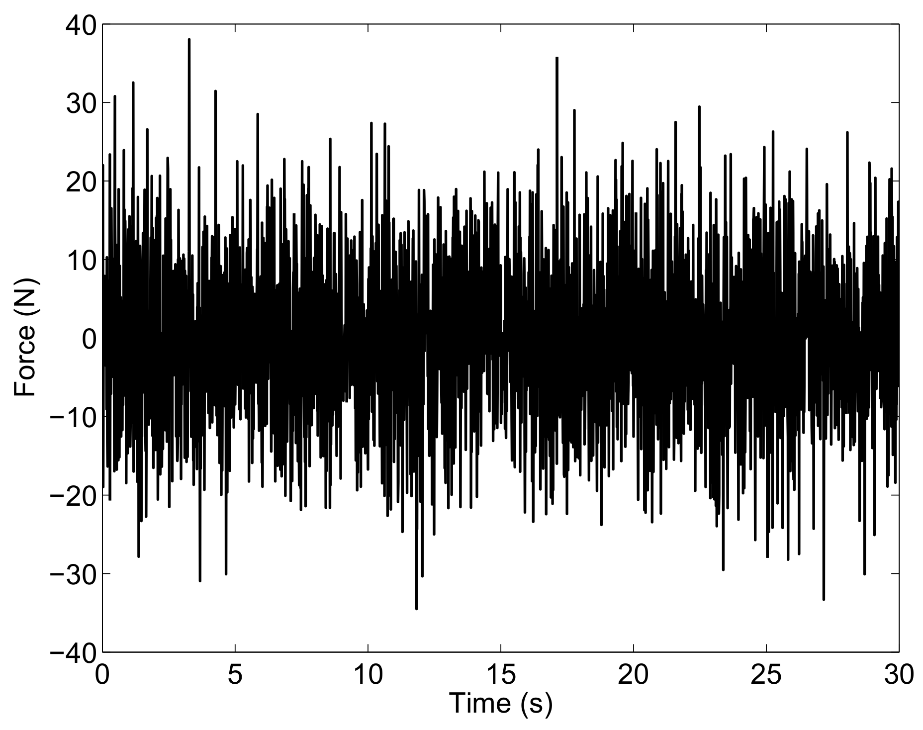
In this numerical example, a time interval of interest equal to (s) is considered, and it is assumed that the input perturbations can be modeled by white noises. The force acting on the vertical degree of freedom of the full-car system is shown in Figure 2 as an example.
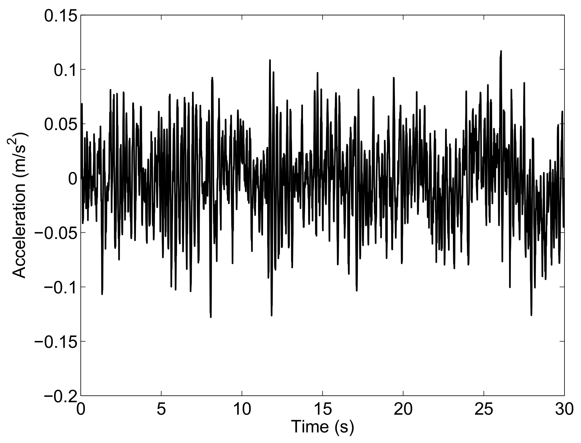
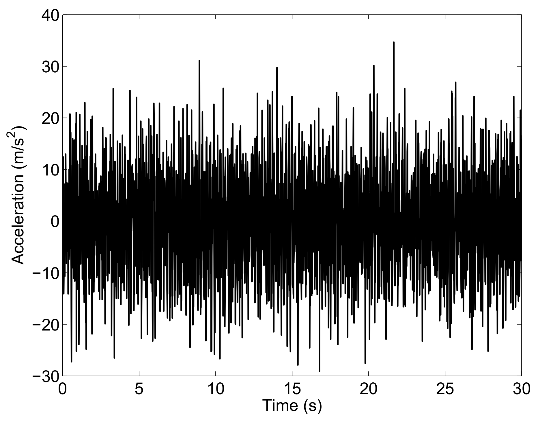
By means of a dynamical simulation carried out in the time domain, one can obtain the generalized displacements, velocities and accelerations of the full-car system corresponding to the external excitations. The vertical acceleration of the chassis of the vehicle is shown in Figure 3 as an example.
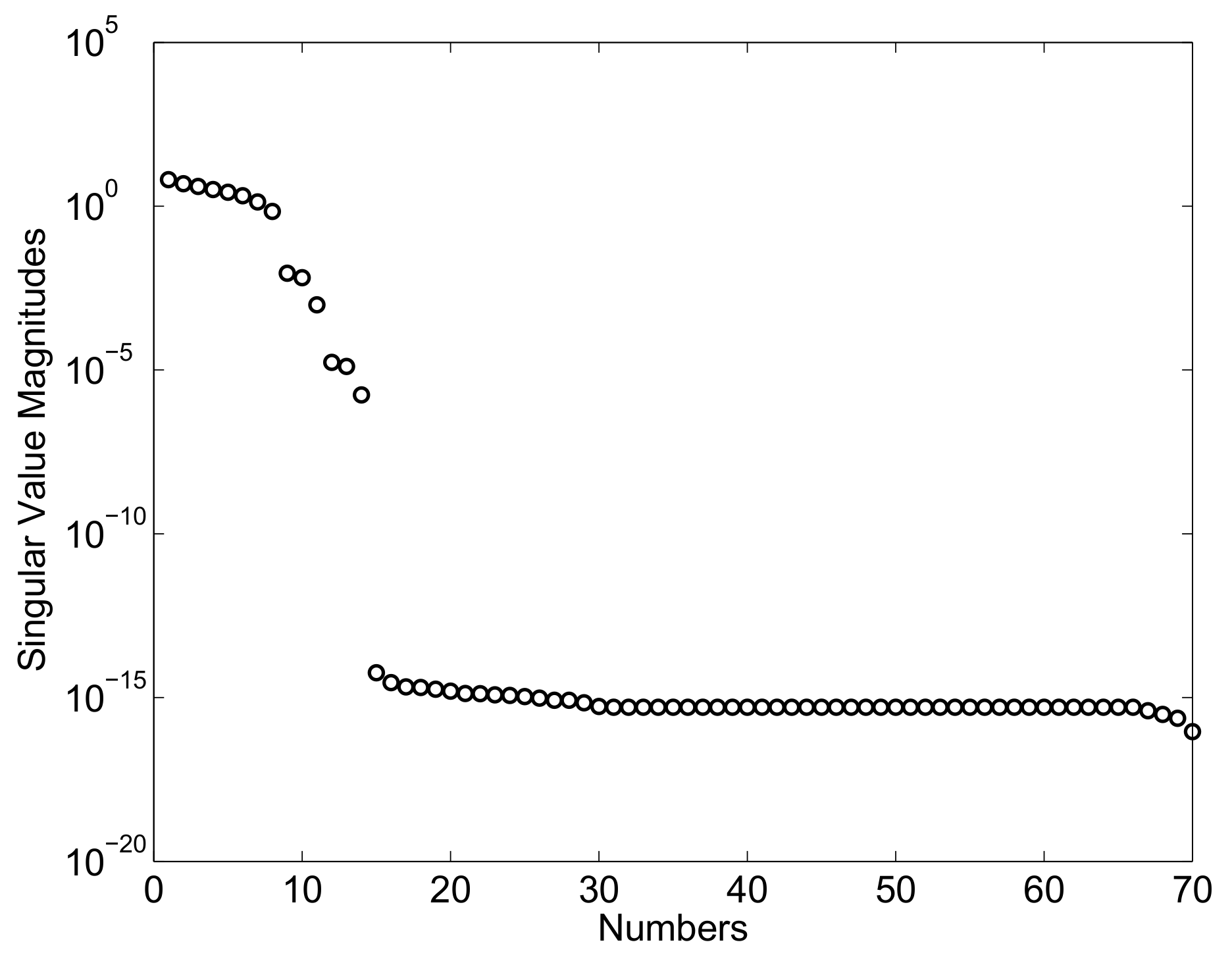
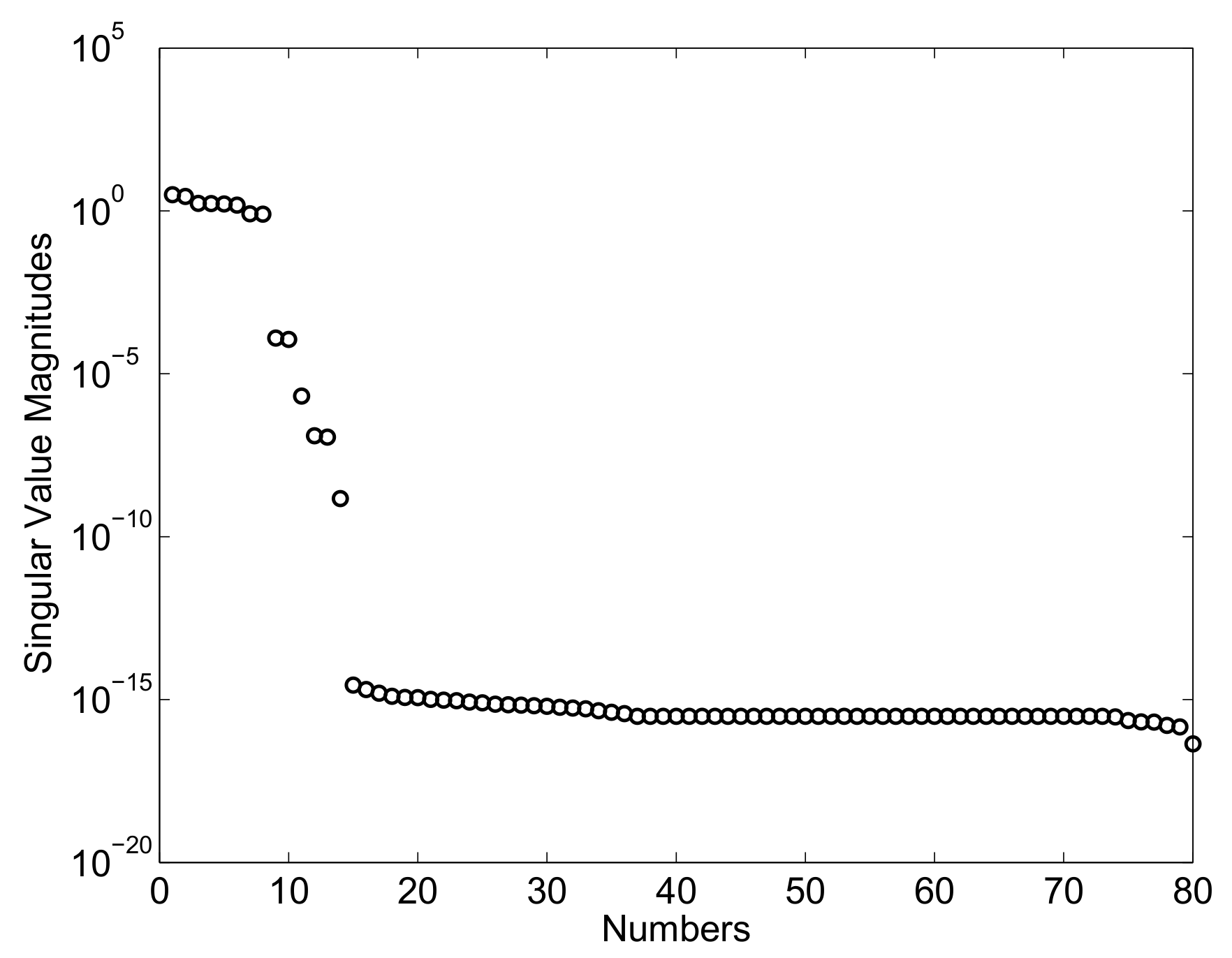
In this numerical example, noise-free data are considered. The use of the system identification procedure applied to the output and input measurements allows for identifying the set of Markov parameters associated with the state-space observed system given by . Subsequently, one can determine the Markov parameters associated with the actual state-space mechanical system indicated with and the Markov parameters associated with the observer gain denoted with . Employing the set of identified Markov parameters, one can assemble the generalized Hankel matrices and required for identifying the state-space model. The generalized matrix obtained in Case Study A features a set of singular values shown in Figure 4.
In this case, a sharp fall in singular values take places in correspondence with the identified model order of the system state-matrix, as shown in Figure 4. By using the identified singular values, a system state-space model can be determined following the identification system procedure discussed in the paper. The identified state-matrix corresponding to the first case study has the following set of eigenvalues:
3.2. Case Study B
In this subsection, the second case study, referred to as Case Study B, is discussed. In this second case study, only four system degrees of freedom corresponding to the vertical motion of the wheels are excited by a set of external perturbations, and the corresponding time responses are recorded. Thus, suppose that one is only capable of measuring the accelerations of the four wheels. Furthermore, assume that only the forces exerted on the vehicle wheels are available as experimental input measurements. In this case, the matrices and are given by:
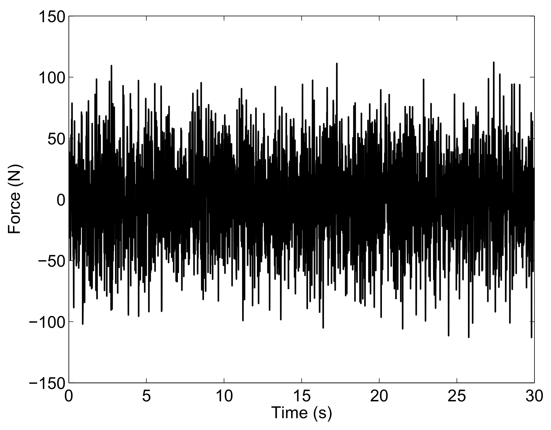
Consider a time span for the dynamic simulations equal to (s), and the external input forces are assumed to be white noises as in the preceding case. The external force applied on the first wheel of the full-car system is shown in the Figure 5 as an example.
The acceleration of the first wheel corresponding to the external excitations of the full-car system is shown in Figure 6 as an example.
In this case, a small amount of artificial noise is used for altering the measured inputs and outputs so that the proposed system identification numerical procedure can be tested in the presence of uncontrollable disturbances. The Hankel matrix singular values obtained in Case Study B are shown in Figure 7.
In this case, the transition from the relatively large singular values associated with the normal modes of the full-car vehicle system to the relatively small singular values representing spurious modes induced by the artificial noise is smoother when compared to the previous case study, as shown in Figure 7. The identified state-matrix corresponding to the second case study has the following set of eigenvalues:
4. Summary, Conclusions and Future Directions of Research
The areas of interest for the research of the authors are the dynamics of rigid and flexible multibody systems, the numerical methods of applied system identification and the theory of nonlinear control [71,72,73,74,75,76,77,78,79,80]. Consequently, the research work of the authors is finalized to the development of new methods for performing accurate analytic modeling, effective numerical parameter identification procedures employing experimental data and nonlinear control optimization algorithms for dynamic models of multibody mechanical systems [81,82,83,84,85,86,87,88,89,90]. In this work, on the other hand, a system identification numerical procedure for identifying the parameters of linear mechanical systems was developed. The system identification numerical procedure is based on a computational approach called the Eigensystem Realization Algorithm (ERA) combined with a numerical algorithm named the Observer/Kalman Filter Identification (OKID) method. In order to illustrate the effectiveness of the numerical procedure developed in this work, the proposed method was used for obtaining the modal parameters of a full-car vehicle model, which represents a standard road vehicle model used for the design of active and semi-active suspension systems. Therefore, the analysis proposed in this investigation can be considered as the first step in the design of a control system for road vehicles. The numerical results found by means of numerical experiments showed a good agreement with the actual modal parameters of the full-car vehicle model even when the input-output measurements are affected by an external source of disturbances. Future investigations will be devoted to performing a systematic comparison of the system identification algorithm developed in this work with other numerical procedures available in the literature.
Author Contributions
This research paper was principally developed by the first author (Carmine Maria Pappalardo). The detailed review carried out by the second author (Domenico Guida) considerably improved the quality of the work.
Conflicts of Interest
The authors declare no conflict of interest.
References
- Udwadia, F.E.; Kalaba, R.E. Analytical Dynamics: A New Approach; Cambridge University Press: New York, NY, USA, 2007. [Google Scholar]
- Villecco, F.; Pellegrino, A. Entropic Measure of Epistemic Uncertainties in Multibody System Models by Axiomatic Design. Entropy 2017, 19, 291. [Google Scholar] [CrossRef]
- Gao, Y.; Villecco, F.; Li, M.; Song, W. Multi-Scale Permutation Entropy Based on Improved LMD and HMM for Rolling Bearing Diagnosis. Entropy 2017, 19, 176. [Google Scholar] [CrossRef]
- Villecco, F.; Pellegrino, A. Evaluation of Uncertainties in the Design Process of Complex Mechanical Systems. Entropy 2017, 19, 475. [Google Scholar] [CrossRef]
- Pappalardo, M.; Villecco, F. Max-Ent in fast belief fusion. In Proceedings of the International Conference Differential Geometry, Dynamical Systems, Bucharest, Romania, 5–7 October 2007; Geometry Balkan Press, University Politehnica Bucharest: Bucharest, Romania, 2008; pp. 154–162. [Google Scholar]
- Formato, A.; Ianniello, D.; Villecco, F.; Lenza, T.L.L.; Guida, D. Design Optimization of the Plough Working Surface by Computerized Mathematical Model. Emir. J. Food Agric. 2017, 29, 36–44. [Google Scholar] [CrossRef]
- Sena, P.; D’Amore, M.; Pappalardo, M.; Pellegrino, A.; Fiorentino, A.; Villecco, F. Studying the Influence of Cognitive Load on Driver’s Performances by a Fuzzy Analysis of Lane Keeping in a Drive Simulation. IFAC Proc. Vol. 2013, 46, 151–156. [Google Scholar] [CrossRef]
- Sena, P.; Attianese, P.; Pappalardo, M.; Villecco, F. FIDELITY: Fuzzy Inferential Diagnostic Engine for on-LIne supporT to phYsicians. In Proceedings of the 4th International Conference on the Development of Biomedical Engineering, Ho Chi Minh City, Vietnam, 8–10 January 2012; pp. 396–400. [Google Scholar]
- Sena, P.; Attianese, P.; Carbone, F.; Pellegrino, A.; Pinto, A.; Villecco, F. A Fuzzy Model to Interpret Data of Drive Performances from Patients with Sleep Deprivation. Comput. Math. Methods Med. 2012, 2012, 868410. [Google Scholar] [CrossRef] [PubMed]
- Zhang, Y.; Li, Z.; Gao, J.; Hong, J.; Villecco, F.; Li, Y. A method for designing assembly tolerance networks of mechanical assemblies. Math. Probl. Eng. 2012, 2012, 513958. [Google Scholar] [CrossRef]
- Sansone, F.; Picerno, P.; Mencherini, T.; Villecco, F.; D’Ursi, A.M.; Aquino, R.P.; Lauro, M.R. Flavonoid Microparticles by Spray-Drying: Influence of Enhancers of the Dissolution Rate on Properties and Stability. J. Food Eng. 2001, 103, 188–196. [Google Scholar] [CrossRef]
- Pellegrino, A.; Villecco, F. Design Optimization of a Natural Gas Substation with Intensification of the Energy Cycle. Math. Probl. Eng. 2010, 2010, 294102. [Google Scholar] [CrossRef]
- Zhai, Y.; Liu, L.; Lu, W.; Li, Y.; Yang, S.; Villecco, F. The Application of Disturbance Observer to Propulsion Control of Sub-mini Underwater Robot. In Proceedings of the ICCSA 2010 International Conference on Computational Science and Its Applications, Fukuoka, Japan, 23–26 March 2010; pp. 590–598. [Google Scholar]
- Ghomshei, M.; Villecco, F.; Porkhial, S.; Pappalardo, M. Complexity in Energy Policy: A Fuzzy Logic Methodology. In Proceedings of the 6th International Conference on Fuzzy Systems and Knowledge Discovery, Tianjin, China, 14–16 August 2009; IEEE: Los Alamitos, CA, USA, 2009; Volume 7, pp. 128–131. [Google Scholar]
- Ghomshei, M.; Villecco, F. Energy Metrics and Sustainability. In Proceedings of the International Conference on Computational Science and Its Applications, Seoul, Korea, 29 June–2 July 2009; pp. 693–698. [Google Scholar]
- Cattani, C.; Mercorelli, P.; Villecco, F.; Harbusch, K. A theoretical multiscale analysis of electrical field for fuel cells stack structures. In International Conference on Computational Science and Its Applications; Springer: Berlin, Heidelberg, 2006; pp. 857–864. [Google Scholar]
- De Simone, M.C.; Rivera, Z.B.; Guida, D. Finite Element Analysis on Squeal-Noise in Railway Applications. FME Trans. 2018, 46, 93–100. [Google Scholar]
- De Simone, M.C.; Guida, D. Identification and Control of a Unmanned Ground Vehicle By using Arduino. UPB Sci. Bull. Ser. D 2018, 80, 141–154. [Google Scholar]
- De Simone, M.C.; Guida, D. Modal Coupling in Presence of Dry Friction. Machines 2018, 6, 8. [Google Scholar] [CrossRef]
- Pappalardo, C.M.; Guida, D. System Identification and Experimental Modal Analysis of a Frame Structure. Eng. Lett. 2018, 26, 56–68. [Google Scholar]
- Guida, D.; Nilvetti, F.; Pappalardo, C.M. Instability Induced by Dry Friction. Int. J. Mech. 2009, 3, 44–51. [Google Scholar]
- Guida, D.; Nilvetti, F.; Pappalardo, C.M. Dry Friction Influence on Cart Pendulum Dynamics. Int. J. Mech. 2009, 3, 31–38. [Google Scholar]
- Ljung, L. System Identification; John Wiley and Sons: Hoboken, NJ, USA, 1999. [Google Scholar]
- Ljung, L. Perspectives on System Identification. Ann. Rev. Contr. 2010, 34, 1–12. [Google Scholar] [CrossRef]
- Forssell, U.; Ljung, L. Closed-Loop Identification Revisited. Automatica 1999, 35, 1215–1241. [Google Scholar] [CrossRef]
- Reynders, E. System Identification Methods for (Operational) Modal Analysis: Review and Comparison. Arch. Comp. Methods Eng. 2012, 19, 51–124. [Google Scholar] [CrossRef]
- Hong, X.; Mitchell, R.J.; Chen, S.; Harris, C.J.; Li, K.; Irwin, G.W. Model Selection Approaches for Non-linear System Identification: A Review. Int. J. Syst. Sci. 2008, 39, 925–946. [Google Scholar] [CrossRef]
- Peeters, B.; De Roeck, G. Stochastic System Identification for Operational Modal Analysis: A Review. J. Dyn. Syst. Meas. Control 2001, 123, 1–9. [Google Scholar] [CrossRef]
- Sands, T.; Kenny, T. Experimental Piezoelectric System Identification. J. Mech. Eng. Autom. 2017, 7, 179–195. [Google Scholar]
- Sands, T. Nonlinear-Adaptive Mathematical System Identification. Computation 2017, 5, 47. [Google Scholar] [CrossRef]
- Sands, T. Space System Identification Algorithms. J. Space Explor. 2017, 6, 138. [Google Scholar]
- Alenany, A.; Mercere, G.; Ramos, J.A. Subspace Identification of 2-D CRSD Roesser Models with Deterministic-Stochastic Inputs: A State Computation Approach. IEEE Trans. Control Syst. Technol. 2017, 25, 1108–1115. [Google Scholar] [CrossRef]
- Ramos, J.A.; Mercere, G. Subspace Algorithms for Identifying Separable-in-denominator 2D Systems with Deterministic–stochastic Inputs. Int. J. Control 2016, 89, 2584–2610. [Google Scholar] [CrossRef]
- Prot, O.; Mercere, G.; Ramos, J. A Null-space-based Technique for the Estimation of Linear-time Invariant Structured State-Space Representations. IFAC Proc. Vol. 2012, 45, 191–196. [Google Scholar] [CrossRef]
- Mercere, G.; Prot, O.; Ramos, J.A. Identification of Parameterized Gray-box State-space Systems: From a Black-box Linear Time-invariant Representation to a Structured One. IEEE Trans. Autom. Control 2014, 59, 2873–2885. [Google Scholar] [CrossRef]
- Nelles, O. Nonlinear System Identification: From Classical Approaches to Neural Networks and Fuzzy Models; Springer Science and Business Media: Berlin, Germany, 2013. [Google Scholar]
- De Simone, M.C.; Russo, S.; Rivera, Z.B.; Guida, D. Multibody model of a UAV in presence of wind fields. In Proceedings of the ICCAIRO 2017—International Conference on Control, Artificial Intelligence, Robotics and Optimization, Prague, Czech Republic, 20–22 May 2017. [Google Scholar]
- De Simone, M.C.; Guida, D. Dry Friction Influence on Structure Dynamics. In Proceedings of the COMPDYN 2015—5th ECCOMAS Thematic Conference on Computational Methods in Structural Dynamics and Earthquake Engineering, Crete, Greece, 25–27 May 2015; pp. 4483–4491. [Google Scholar]
- Guida, D.; Nilvetti, F.; Pappalardo, C.M. Parameter Identification of a Two Degrees of Freedom Mechanical System. Int. J. Mech. 2009, 3, 23–30. [Google Scholar]
- Guida, D.; Pappalardo, C.M. Sommerfeld and Mass Parameter Identification of Lubricated Journal Bearing. WSEAS Trans. Appl. Theor. Mech. 2009, 4, 205–214. [Google Scholar]
- Strano, S.; Terzo, M. Actuator Dynamics Compensation for Real-time Hybrid Simulation: An Adaptive Approach by means of a Nonlinear Estimator. Nonlinear Dyn. 2016, 85, 2353–2368. [Google Scholar] [CrossRef]
- Strano, S.; Terzo, M. Accurate State Estimation for a Hydraulic Actuator via a SDRE Nonlinear Filter. Mech. Syst. Signal Process. 2016, 75, 576–588. [Google Scholar] [CrossRef]
- Russo, R.; Strano, S.; Terzo, M. Enhancement of Vehicle Dynamics via an Innovative Magnetorheological Fluid Limited Slip Differential. Mech. Syst. Signal Process. 2016, 70, 1193–1208. [Google Scholar] [CrossRef]
- Strano, S.; Terzo, M. A SDRE-based Tracking Control for a Hydraulic Actuation System. Mech. Syst. Signal Process. 2015, 60, 715–726. [Google Scholar] [CrossRef]
- Marques, F.; Souto, A.P.; Flores, P. On the Constraints Violation in Forward Dynamics of Multibody Systems. Multibody Syst. Dyn. 2017, 39, 385–419. [Google Scholar] [CrossRef]
- Liu, C.; Tian, Q.; Hu, H.; Garcia-Vallejo, D. Simple Formulations of Imposing Moments and Evaluating Joint Reaction Forces for Rigid-flexible Multibody Systems. Nonlinear Dyn. 2012, 69, 127–147. [Google Scholar] [CrossRef]
- Tian, Q.; Chen, L.P.; Zhang, Y.Q.; Yang, J. An Efficient Hybrid Method for Multibody Dynamics Simulation based on Absolute Nodal Coordinate Formulation. J. Comput. Nonlinear Dyn. 2009, 4, 021009. [Google Scholar] [CrossRef]
- Cammarata, A.; Calio, I.; Greco, A.; Lacagnina, M.; Fichera, G. Dynamic Stiffness Model of Spherical Parallel Robots. Sound Vib. 2016, 384, 312–324. [Google Scholar] [CrossRef]
- Cammarata, A. Unified Formulation for the Stiffness Analysis of Spatial Mechanisms. Mech. Mach. Theory 2016, 105, 272–284. [Google Scholar] [CrossRef]
- Cammarata, A.; Angeles, J.; Sinatra, R. The Dynamics of Parallel Schonflies Motion Generators: The Case of a Two-limb System. Proc. Inst. Mech. Eng. Part I J. Syst. Control Eng. 2009, 223, 29–52. [Google Scholar] [CrossRef]
- Lan, P.; Shabana, A.A. Rational Finite Elements and Flexible Body Dynamics. J. Vib. Acoust. 2010, 132, 041007. [Google Scholar] [CrossRef]
- Hu, W.; Tian, Q.; Hu, H. Dynamic Simulation of Liquid-filled Flexible Multibody Systems via Absolute Nodal Coordinate Formulation and SPH Method. Nonlinear Dyn. 2014, 75, 653–671. [Google Scholar] [CrossRef]
- Liu, C.; Tian, Q.; Hu, H. Dynamics of a Large Scale Rigid–flexible Multibody System Composed of Composite Laminated Plates. Multibody Syst. Dyn. 2011, 26, 283–305. [Google Scholar] [CrossRef]
- Patel, M.; Orzechowski, G.; Tian, Q.; Shabana, A.A. A New Multibody System Approach for Tire Modeling using ANCF Finite Elements. Proc. Inst. Mech. Eng. Part K J. Multibody Dyn. 2016, 230, 69–84. [Google Scholar] [CrossRef]
- Udwadia, F.E.; Wanichanon, T. On General Nonlinear Constrained Mechanical Systems. Numer. Algebra Control Optim. 2013, 3, 425–443. [Google Scholar] [CrossRef]
- Schutte, A.; Udwadia, F. New Approach to the Modeling of Complex Multibody Dynamical Systems. J. Appl. Mech. 2011, 78, 021018. [Google Scholar] [CrossRef]
- Roman, R.C.; Radac, M.B.; Precup, R.E.; Petriu, E.M. Virtual Reference Feedback Tuning of Model-Free Control Algorithms for Servo Systems. Machines 2017, 5, 25. [Google Scholar] [CrossRef]
- Precup, R.E.; David, R.C.; Szedlak-Stinean, A.I.; Petriu, E.M.; Dragan, F. An Easily Understandable Grey Wolf Optimizer and Its Application to Fuzzy Controller Tuning. Algorithms 2017, 10, 68. [Google Scholar] [CrossRef]
- Radac, M.B.; Precup, R.E. Data-Driven Model-Free Slip Control of Anti-Lock Braking Systems using Reinforcement Q-Learning. Neurocomputing 2018, 275, 317–329. [Google Scholar] [CrossRef]
- Radac, M.B.; Precup, R.E.; Roman, R.C. Data-Driven Model Reference Control of MIMO Vertical Tank Systems with Model-Free VRFT and Q-Learning. ISA Trans. 2018, 73, 22–30. [Google Scholar] [CrossRef] [PubMed]
- Pozna, C.; Precup, R.E. On a Translated Frame-Based Approach to Geometric Modeling of Robots. Robot. Autom. Syst. 2017, 91, 49–58. [Google Scholar] [CrossRef]
- Sharifzadeh, M.; Farnam, A.; Senatore, A.; Timpone, F.; Akbari, A. Delay-Dependent Criteria for Robust Dynamic Stability Control of Articulated Vehicles. In Proceedings of the International Conference on Robotics in Alpe-Adria Danube Region, Turin, Italy, 21–23 June 2017; pp. 424–432. [Google Scholar]
- Sharifzadeh, M.; Timpone, F.; Farnam, A.; Senatore, A.; Akbari, A. Tyre-road Adherence Conditions Estimation for Intelligent Vehicle Safety Applications. In Advances in Italian Mechanism Science, Mechanisms and Machine Science; Springer: Cham, Switzerlane, 2017; Volume 47, pp. 389–398. [Google Scholar]
- Pennestrí, E.; Valentini, P.P.; De Falco, D. An Application of the Udwadia-Kalaba Dynamic Formulation to Flexible Multibody Systems. J. Frankl. Inst. 2010, 347, 173–194. [Google Scholar] [CrossRef]
- De Falco, D.; Pennestrí, E.; Vita, L. Investigation of the Influence of Pseudoinverse Matrix Calculations on Multibody Dynamics Simulations by means of the Udwadia-Kalaba Formulation. J. Aerosp. Eng. 2009, 22, 365–372. [Google Scholar] [CrossRef]
- Nachbagauer, K.; Oberpeilsteiner, S.; Sherif, K.; Steiner, W. The Use of the Adjoint Method for Solving Typical Optimization Problems in Multibody Dynamics. J. Comput. Nonlinear Dyn. 2015, 10, 061011. [Google Scholar] [CrossRef]
- Oberpeilsteiner, S.; Lauss, T.; Nachbagauer, K.; Steiner, W. Optimal Input Design for Multibody Systems by using an Extended Adjoint Approach. Multibody Syst. Dyn. 2017, 40, 43–54. [Google Scholar] [CrossRef] [PubMed]
- Pappalardo, C.M.; Guida, D. Adjoint-based Optimization Procedure for Active Vibration Control of Nonlinear Mechanical Systems. J. Dyn. Syst. Meas. Control 2017, 139, 081010. [Google Scholar] [CrossRef]
- Pappalardo, C.M.; Guida, D. Control of Nonlinear Vibrations using the Adjoint Method. Meccanica 2017, 52, 2503–2526. [Google Scholar] [CrossRef]
- Juang, J.N.; Phan, M.Q. Identification and Control of Mechanical Systems; Cambridge University Press: New York, NY, USA, 2001. [Google Scholar]
- Quatrano, A.; De Simone, M.C.; Rivera, Z.B.; Guida, D. Development and implementation of a control system for a retrofitted CNC machine by using Arduino. FME Trans. 2017, 45, 565–571. [Google Scholar] [CrossRef]
- Concilio, A.; De Simone, M.C.; Rivera, Z.B.; Guida, D. A new semi-active suspension system for racing vehicles. FME Trans. 2017, 45, 578–584. [Google Scholar] [CrossRef]
- Ruggiero, A.; De Simone, M.C.; Russo, D.; Guida, D. Sound Pressure Measurement of Orchestral Instruments in the Concert Hall of a Public School. Int. J. Circuits Syst. Signal Process. 2016, 10, 75–81. [Google Scholar]
- Kulkarni, S.; Pappalardo, C.M.; Shabana, A.A. Pantograph/Catenary Contact Formulations. J. Vib. Acoust. 2017, 139, 011010. [Google Scholar] [CrossRef]
- Guida, D.; Pappalardo, C.M. Control Design of an Active Suspension System for a Quarter-Car Model with Hysteresis. J. Vib. Eng. Technol. 2015, 3, 277–299. [Google Scholar]
- Guida, D.; Pappalardo, C.M. A New Control Algorithm for Active Suspension Systems Featuring Hysteresis. FME Trans. 2013, 41, 285–290. [Google Scholar]
- Pappalardo, C.M.; Guida, D. On the Use of Two-dimensional Euler Parameters for the Dynamic Simulation of Planar Rigid Multibody Systems. Arch. Appl. Mech. 2017, 87, 1647–1665. [Google Scholar] [CrossRef]
- Pappalardo, C.M.; Wang, T.; Shabana, A.A. On the Formulation of the Planar ANCF Triangular Finite Elements. Nonlinear Dyn. 2017, 89, 1019–1045. [Google Scholar] [CrossRef]
- Pappalardo, C.M.; Wang, T.; Shabana, A.A. Development of ANCF Tetrahedral Finite Elements for the Nonlinear Dynamics of Flexible Structures. Nonlinear Dyn. 2017, 89, 2905–2932. [Google Scholar] [CrossRef]
- Pappalardo, C.M.; Guida, D. On the Lagrange Multipliers of the Intrinsic Constraint Equations of Rigid Multibody Mechanical Systems. Arch. Appl. Mech. 2017, 1–33. [Google Scholar] [CrossRef]
- De Simone, M.C.; Guida, D. On the Development of a Low Cost Device for Retrofitting Tracked Vehicles for Autonomous Navigation. In Proceedings of the AIMETA 2017—XXIII Conference of The Italian Association of Theoretical and Applied Mechanics, Salerno, Italy, 4–7 September 2017. [Google Scholar]
- Ruggiero, A.; Affatato, S.; Merola, M.; De Simone, M.C. FEM Analysis of Metal on UHMWPE Total Hip Prosthesis During Normal Walking Cycle. In Proceedings of the AIMETA 2017—XXIII Conference of The Italian Association of Theoretical and Applied Mechanics, Salerno, Italy, 4–7 September 2017. [Google Scholar]
- Pappalardo, C.M.; Yu, Z.; Zhang, X.; Shabana, A.A. Rational ANCF Thin Plate Finite Element. J. Comput. Nonlinear Dyn. 2016, 11, 051009. [Google Scholar] [CrossRef]
- Pappalardo, C.M.; Zhang, Z.; Shabana, A.A. Use of Independent Volume Parameters in the Development of New Large Displacement ANCF Triangular Plate/Shell Elements. Nonlinear Dyn. 2018, 1–32. [Google Scholar] [CrossRef]
- Pappalardo, C.M.; Patel, M.D.; Tinsley, B.; Shabana, A.A. Contact Force Control in Multibody Pantograph/Catenary Systems. Proc. Inst. Mech. Eng. Part K J. Multibody Dyn. 2016, 230, 307–328. [Google Scholar] [CrossRef]
- Guida, D.; Pappalardo, C.M. Forward and Inverse Dynamics of Nonholonomic Mechanical Systems. Meccanica 2014, 49, 1547–1559. [Google Scholar] [CrossRef]
- Pappalardo, C.M.; Wallin, M.; Shabana, A.A. A New ANCF/CRBF Fully Parametrized Plate Finite Element. J. Comput. Nonlinear Dyn. 2017, 12, 031008. [Google Scholar] [CrossRef]
- Pappalardo, C.M. A Natural Absolute Coordinate Formulation for the Kinematic and Dynamic Analysis of Rigid Multibody Systems. Nonlinear Dyn. 2015, 81, 1841–1869. [Google Scholar] [CrossRef]
- Pappalardo, C.M.; Guida, D. Dynamic Analysis of Planar Rigid Multibody Systems modeled using Natural Absolute Coordinates. Appl. Comput. Mech. 2018, in press. [Google Scholar]
- Pappalardo, C.M. Modelling Rigid Multibody Systems using Natural Absolute Coordinates. J. Mech. Eng. Ind. Des. 2014, 3, 24–38. [Google Scholar]
Figure 1.
Full-car model.
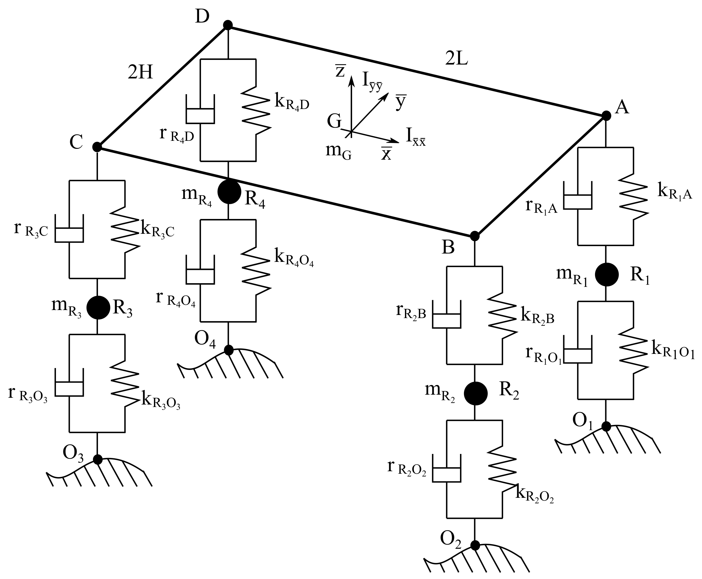
Figure 2.
Vertical input force on the chassis: Case Study A.

Figure 3.
Vertical output acceleration of the chassis: Case Study A.

Figure 4.
Singular value magnitudes: Case Study A.

Figure 5.
Vertical input force on the first wheel: Case Study B.

Figure 6.
Vertical output acceleration of the first wheel: Case Study B.

Figure 7.
Singular value magnitudes: Case Study B.
© 2018 by the authors. Licensee MDPI, Basel, Switzerland. This article is an open access article distributed under the terms and conditions of the Creative Commons Attribution (CC BY) license (http://creativecommons.org/licenses/by/4.0/).
Share and Cite
MDPI and ACS Style
Pappalardo, C.M.; Guida, D. System Identification Algorithm for Computing the Modal Parameters of Linear Mechanical Systems. Machines 2018, 6, 12. https://doi.org/10.3390/machines6020012
AMA Style
Pappalardo CM, Guida D. System Identification Algorithm for Computing the Modal Parameters of Linear Mechanical Systems. Machines. 2018; 6(2):12. https://doi.org/10.3390/machines6020012
Chicago/Turabian StylePappalardo, Carmine Maria, and Domenico Guida. 2018. "System Identification Algorithm for Computing the Modal Parameters of Linear Mechanical Systems" Machines 6, no. 2: 12. https://doi.org/10.3390/machines6020012
Note that from the first issue of 2016, this journal uses article numbers instead of page numbers. See further details here.