Use of the Adjoint Method for Controlling the Mechanical Vibrations of Nonlinear Systems


Department of Industrial Engineering, University of Salerno, Via Giovanni Paolo II, 132, 84084 Fisciano, Italy
*
Author to whom correspondence should be addressed.
Machines 2018, 6(2), 19; https://doi.org/10.3390/machines6020019
Submission received: 28 March 2018
/
Revised: 25 April 2018
/
Accepted: 2 May 2018
/
Published: 4 May 2018
(This article belongs to the Special Issue Advanced Control Systems and Optimization Techniques)
Abstract
:In this work, the analytical derivation and the computer implementation of the adjoint method are described. The adjoint method can be effectively used for solving the optimal control problem associated with a large class of nonlinear mechanical systems. As discussed in this investigation, the adjoint method represents a broad computational framework, rather than a single numerical algorithm, in which the control problem for nonlinear dynamical systems can be effectively formulated and implemented employing a set of advanced analytical methods as well as an array of well-established numerical procedures. A detailed theoretical derivation and a comprehensive description of the numerical algorithm suitable for the computer implementation of the methodology used for performing the adjoint analysis are provided in the paper. For this purpose, two important cases are analyzed in this work, namely the design of a feedforward control scheme and the development of a feedback control architecture. In this investigation, the control problem relative to the mechanical vibrations of a nonlinear oscillator characterized by a generalized Van der Pol damping model is considered in order to illustrate the effectiveness of the computational algorithm based on the adjoint method by means of numerical experiments.
1. Introduction
This paper is focused on the development of an adjoint-based analytical and computational framework for the optimal design of open-loop and closed-loop control laws suitable for controlling nonlinear mechanical systems. In this section, background material, a concise literature review, the formulation of the problem of interest for this study, the scope and the contributions of this investigation, and the organization of the manuscript are provided.
1.1. Background and Significance
In different areas of structural and mechanical engineering, the study of the mechanical behavior of dynamical systems having a nonlinear nature represents an important field of research [1,2]. As discussed in detail in the scientific literature, this problem is relevant especially in the case of complex engineering systems in which the final design solution represents an engineering approximation subjected to a certain degree of uncertainty [3,4,5,6,7,8,9,10,11,12,13,14,15,16,17]. In order to develop effective control actions for controlling the dynamic evolution of a general nonlinear mechanical system, appropriate formulation procedures and computational strategies are needed. Therefore, the first step necessary for the development of a new control strategy for a given mechanical system is to construct a reliable dynamic model of the system itself that is able to correctly capture its intrinsic nonlinear physics. Afterward, the design problem concerning the development of a control strategy for the nonlinear mechanical system under consideration can be addressed using several approaches and methodologies available in the literature. For example, the classical control methods are based on the linearization of the dynamic equations of the mechanical system under examination. Such methods lead to a loss of information on the complex nonlinear dynamic behavior and work properly only when the time response of the mechanical system at hand evolves around a fixed point of the state space or in the proximity of a prescribed trajectory. However, this is not the case of several mechanical systems employed in engineering applications in which a fully nonlinear dynamic behavior is found and, therefore, more complex control strategies are required.
1.2. Literature Review
In engineering applications, the analysis and the synthesis of machines and structures subjected to nonlinear vibrations represent an important topic of research. Several different energy sources can induce undesired mechanical vibrations of a given structural system, which, in turn, can be dangerous for the system integrity and can lead to a progressive deterioration of the system performance. Consequently, in numerous industrial applications, the vibration control problem represents a fundamental issue. In order to solve this important problem, different analytical approaches, computational methods, and experimental solutions have been extensively developed and tested in recent years. For instance, the methods based on the State-Dependent Riccati Equation (SDRE), the feedback linearization method, the sliding mode control approach, and nonlinear control methods based on the control-Lyapunov function represent effective control strategies suitable for solving the vibration control problem associated with a nonlinear mechanical system [18,19,20,21,22,23,24,25,26,27,28,29]. Moreover, the vibration control problem is particularly challenging in the case of rigid-flexible multibody mechanical systems. A multibody system is a special type of mechanical system characterized by a set of rigid bodies, deformable components, kinematic joints, force elements, force fields, electromechanical sensors, and control actuators [30,31,32,33,34,35,36,37]. Among the others, mechanisms and machines, flexible robotic manipulators, ground vehicles, aerospace structures, and biomechanical systems are examples of rigid-flexible multibody mechanical systems [38,39,40,41,42,43]. In order to solve the vibration control problem associated with a multibody mechanical system, the correct analytical formulation and the consistent numerical solution of the equations of motion represent a fundamental step of primary importance that is a current topic of research [44,45,46,47,48,49,50,51]. To this end, several multibody formulation approaches based on the finite element method have been recently developed for modelling flexible continuum bodies that undergo large reference displacements and large deformations [52,53,54,55,56,57,58,59]. In particular, the simple algorithms based on the linearization of the dynamic equations are not suitable for controlling the nonlinear behavior of a flexible multibody mechanical system and more advanced control approaches and numerical procedures are required [60,61,62,63,64,65].
1.3. Formulation of the Problem of Interest for this Study
In order to face the challenges associated with the nonlinear control problem, the adjoint method was originally devised in the field of computational fluid dynamics [66,67]. The adjoint method represents a wide computational procedure, rather than a single method, in which the control problem of nonlinear mechanical systems is analyzed by using the optimal control theory and an approximate solution of the resulting set of differential-algebraic equations can be obtained employing a broad variety of numerical procedures [68,69]. For this purpose, the discrete-time solution of the continuous-time adjoint equations can be achieved by the formulation of a set of archetypical sub-problems that can be treated with some mathematical techniques already developed and optimized in the field of numerical analysis [70]. For example, the adjoint method for solving the nonlinear optimal control problem has been applied in different engineering areas such as structural design and shape optimization, structural mechanics, electromagnetics, fluid kinetics, and the stabilization of business cycles of finance agents [71,72,73,74]. Since this process is not unique and, therefore, several valid options are available, there is the need for defining in a clear perspective the structure of the adjoint method in order to facilitate the development of a more general computational framework in which the adjoint equations can be effectively formulated and solved.
1.4. Scope and Contributions of this Investigation
The research presented in this work represents an attempt to address the important nonlinear control problem by developing a general computational procedure based on the adjoint method. For this purpose, this investigation is focused on a general adjoint-based approach that can be tested in a virtual environment by means of dynamical simulations and can be subsequently implemented in a control system based on the feedforward and feedback control paradigms. Thus, the purpose of this paper is to use the analytical background to formulate the adjoint equations and, at the same time, to propose a viable path that can be followed step-by-step for the numerical solutions of the adjoint equations employing a reliable set of pre-established computational algorithms. On the other hand, in order to demonstrate the effectiveness and the feasibility of the adjoint-based approach for obtaining nonlinear control laws suitable for solving the optimal control problem for a general class of mechanical systems, the vibration control problem of a nonlinear oscillator is considered in this investigation as an illustrative example. As will be shown in future investigations, the nonlinear control method developed in this paper can be extended to the class of multibody mechanical systems by formulating and solving the adjoint equations for a differential-algebraic set of dynamic equations.
This paper is part of a wider research plan that deals with the use of analytical methods and numerical techniques for solving the optimal control problem associated with the dynamic behavior of nonlinear mechanical systems. In such regard, the adjoint equations are analytically formulated in this work considering a general case of a nonlinear dynamical system. Afterward, an iterative procedure for performing the nonlinear optimization of the desired control laws is developed in this investigation. In the computational procedure elaborated in this study, the fourth-order explicit Adams–Bashforth method is used for numerically solving the direct dynamic problem as well as the inverse adjoint problem; the conjugate gradient method based on the Fletcher–Reeves numerical scheme is employed in the formulation of the line search strategy for computing the minimum of the cost functional; the golden section algorithm is implemented for bracketing the search interval of the minimum and for computing the line parameter corresponding to the minimum of the cost function. As demonstrated by using the numerical results obtained in the paper, the approach developed in this investigation allows for deriving effective open-loop and closed-loop control actions.
1.5. Organization of the Manuscript
The structure of this manuscript can be summarized as follows. In Section 2, the analytical derivation of the adjoint equations and their application to the optimal control problem are discussed. In particular, the optimal design of control actions based the open-loop and closed-loop strategies are analyzed in this section. In Section 3, the computational steps necessary for obtaining an optimal numerical solution of the adjoint equations are illustrated in the case of a simple demonstrative example. For this purpose, the problem of the vibration reduction of a nonlinear oscillator is considered in the paper for demonstrating the computer implementation of the adjoint-based approach. In Section 4, the summary of this investigation, the conclusions drawn in this paper, and some indications on the future directions of research are provided.
2. Mathematical Background
In this section, background material on the analytical formulation of the adjoint equations is reported. Subsequently, the principal steps for numerically solving the adjoint equations by means of a general solution framework are described. In order to achieve this goal, two general cases are considered. The first case is the design of an optimal open-loop controller, while the second case is the design of an optimal closed-loop controller.
2.1. Adjoint Equations for Constructing an Optimal Open-Loop Controller
In this subsection, the adjoint equations for the optimal construction of a feedforward control action are discussed. A feedforward control action is an open-loop control law characterized by a set of explicit functions of time [75,76]. In the case of the design of an optimal open-loop controller, consider a system of n differential equations featuring a nonlinear structure that mathematically describes a dynamical system:
where t is the continuous time variable, is a vector of dimension n that defines the system state, is a vector of dimension n denoting the initial conditions, is a vector of dimension n representing the system state function, is a vector of dimension that stands for the open-loop control action, and is a vector of dimension representing the external inputs that are uncontrollable. In the case of the derivation of an optimal open-loop controller, one can assume a cost functional defined as:
where T is a specified time horizon, is called terminal cost function, and is referred to as the current cost function [77]. In the case of the design of an optimal open-loop controller, one can introduce an augmented cost functional employing the mathematical expressions of the system state-space equations of motion (1) and the cost functional (2) by means of an adjoining process as follows:
where identifies the adjoint state vector. On the other hand, consider the Hamiltonian function defined as:
It can be proved that an optimal feedforward control action can be obtained in correspondence of an unconstrained minimum of the Hamiltonian function [78]. To this end, one can write:
The augmented cost functional (3) can be rewritten employing the integration by parts process as:
The variation of the augmented cost functional (6) yields:
One can considerably simplify the mathematical form of the first variation of the augmented cost functional (7) by introducing the following definitions:
where is the state matrix of dimensions obtained by linearizing the system state function around the current system state , is the input influence matrix of dimensions obtained by linearizing the system state function around the current open-loop control action vector , is the perturbation vector having dimension n of the terminal cost function h referred to the system state , is the perturbation vector having dimension n of the current cost function g referred to the system state , and is the perturbation vector having dimension of the current cost function g referred to the open-loop control action vector . Therefore, the first variation of the augmented cost functional can be rewritten as:
Assuming that the system initial state is fixed and considering a given time horizon T, the nonlinear set of equations that identify an optimal feedforward controller can be derived as follows:
2.2. Adjoint Equations for Constructing an Optimal Closed-Loop Controller
In this subsection, the adjoint equations for the optimal derivation of a feedback control action are illustrated. A feedback control action is a closed-loop control law characterized by an explicit function of the system state [80,81]. In the case of the design of an optimal closed-loop controller, consider a system of n differential equations having a nonlinear structure, which mathematically represents a mechanical system:
where t is the continuous time variable, is a vector of dimension n that indicates the system state, is a vector of dimension n denoting the initial conditions, is a vector of dimension n representing the system state function, is a vector of dimension that describes the closed-loop control action defined in terms of a set of constant control parameters grouped in the parameter vector having dimension , and is a vector of dimension representing the external inputs that are uncontrollable. In the case of the construction of an optimal closed-loop controller, one can consider a cost functional denoted with and defined as:
where T is a given time interval, is referred to as the terminal cost function, and is called the current cost function [82]. In the case of the design of an optimal closed-loop controller, one can define an augmented cost functional using the analytical forms of the system equations of motion (11) and the cost functional (12) considering an adjoining process as follows:
where identifies the adjoint state vector. On the other hand, consider the Hamiltonian function given by:
One can demonstrate that an optimal set of control parameters associated with the feedback controller corresponds to an unconstrained minimum of the Hamiltonian function [83]. For this purpose, one can define:
The augmented cost functional (13) can be reformulated using the integration by parts rule as:
The variation of the augmented cost functional (16) produces:
One can substantially simplify the analytical form of the first variation of the augmented cost functional (17) by introducing the following definitions:
where is the state matrix of dimensions obtained by linearizing the system state function around the current system state , is the input influence matrix of dimensions obtained by linearizing the system state function around the current closed-loop control parameter vector , is the perturbation vector having dimension n of the terminal cost function h referred to the system state , is the perturbation vector having dimension n of the current cost function g referred to the system state , and is the perturbation vector of dimension of the current cost function g referred to the closed-loop control parameter vector . Thus, the first variation of the augmented cost functional can be rewritten as follows:
Considering a given vector of initial conditions and assuming a fixed time interval T, the nonlinear set of equations that defines an optimal feedback controller can be obtained as follows:
The resulting set of integro-differential-algebraic equations given by Equation (20) constitutes the adjoint equations and forms an integro-differential-algebraic nonlinear two-point boundary value problem representing the necessary conditions associated with an optimal feedback control action [84].
2.3. Iterative Adjoint-Based Computational Optimization Algorithm
In this subsection, the principal computational steps of the computer implementation of the adjoint equations are described. To this end, a numerical method for the derivation of an optimal open-loop controller as well as the construction of an optimal closed-loop control action are considered. In both the adjoint-based control optimization procedure and the adjoint-based parameter optimization procedure, a line search approach is used for searching for the minimum of the cost functional that corresponds to an optimal control law. For this purpose, in the case of the research of an optimal feedforward control action, the following structure of the control input can be assumed for implementing the iterative line search algorithm:
where is the optimal control force vector at the iteration k, identifies the direction of the research of the minimum, and is a dimensionless parameter to be determined by means of a minimization process. On the other hand, in the case of the research of an optimal feedback controller, one can write in a similar way:
where is the optimal control parameter vector at the iteration k. There are several useful strategies available in the literature for selecting an optimal direction of research in the iterative minimization algorithm [85]. For instance, considering the conjugate gradient method, one can assume the following direction vector:
where the parameter can be found using the following formula based on the Fletcher–Reeves method:
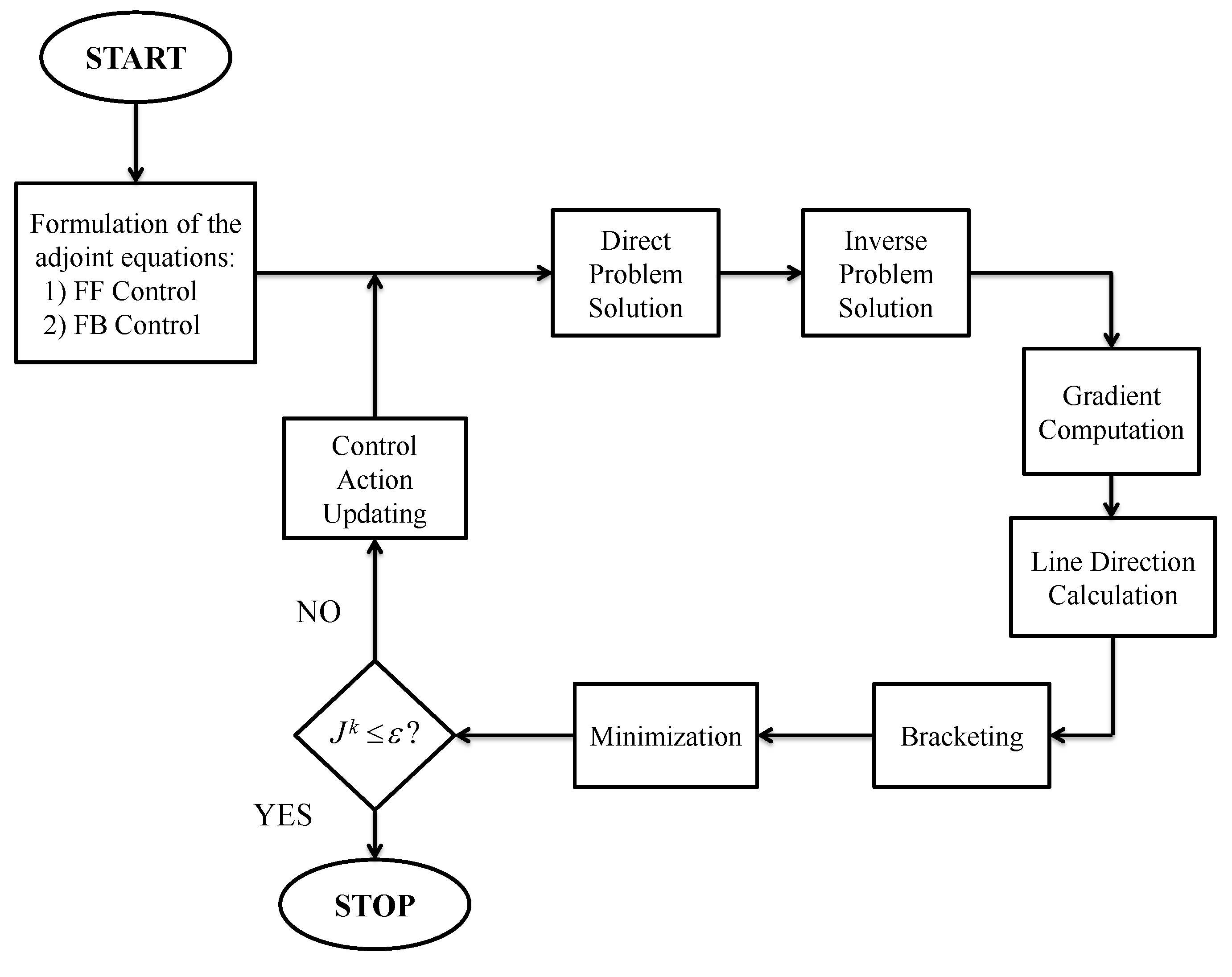
where denotes the gradient vector of the cost functional, which can be obtained from the third equation of the systems (10) and (20), respectively, for an optimal feedforward and an optimal feedback control scheme. The dimensionless parameter , on the other hand, can be calculated using a standard minimization procedure for one-dimensional functions preceded by a process of bracketing of the interval in which a local minimum is collocated. In order to obtain the gradient of the cost functional at a given step k of the iterative procedure, one needs to solve the system equations of motion and, subsequently, the system adjoint equations that represent the first two equations of the systems (10) and (20). These two computational steps are respectively called solutions of the direct problem and solution of the inverse problem. The complete process continues iteratively until a tolerance is reached for the variation of the minimum of the cost functional obtained numerically. A schematic representation of the iterative computational procedure used for solving the adjoint equations is represented in Figure 1.
In Figure 1, denotes the tolerance set for the iterative minimization of the cost function . The computational procedure described in this subsection can be used for the computer implementation the adjoint method, which leads to a numerical solution for an optimal open-loop controller and an optimal closed-loop controller. In particular, the flowchart illustrated in Figure 1 describes the principal steps necessary for the computer implementation of the adjoint approach. It is important to note that all the computational steps of the adjoint-based iterative procedure can be implemented employing standard numerical methods. For this purpose, the solution of both the direct and inverse problems can be performed using the explicit and/or implicit Runge–Kutta algorithms as well as the explicit and/or implicit linear multistep schemes. Several numerical methods are also suitable for obtaining the line direction used in the search algorithm such as, for example, the simple steepest descent approach as well as the more advanced conjugate gradient algorithms and the quasi-Newton methods. Furthermore, both the bracketing of the minimum and the minimization of the cost function can be carried out employing the Fibonacci search approach, the golden section search algorithm, and the Brent search method. In this paper, on the other hand, the fourth-order explicit Adams–Bashforth method was used for solving both the direct and the inverse problems, the conjugate gradient method based on the Fletcher–Reeves algorithm was employed for computing the gradient-based search direction at each iteration of the minimization procedure, and the golden section approach was implemented for accomplishing both the bracketing of the minimum and the minimization of the cost function. As illustrated in the numerical result section of this investigation, the approach developed in this paper produces feedforward and feedback control laws that are efficient and effective.
3. Numerical Results and Discussion
In this section, a demonstrative example is used for testing the effectiveness of the analytical methods developed in this paper employing dynamical simulations. This section is also used for illustrating the main steps of the numerical implementation of the adjoint-based approach. To this end, the performance of the adjoint equations for the design of optimal feedforward and feedback controllers are analyzed below.
3.1. Description of the Demonstrative Example
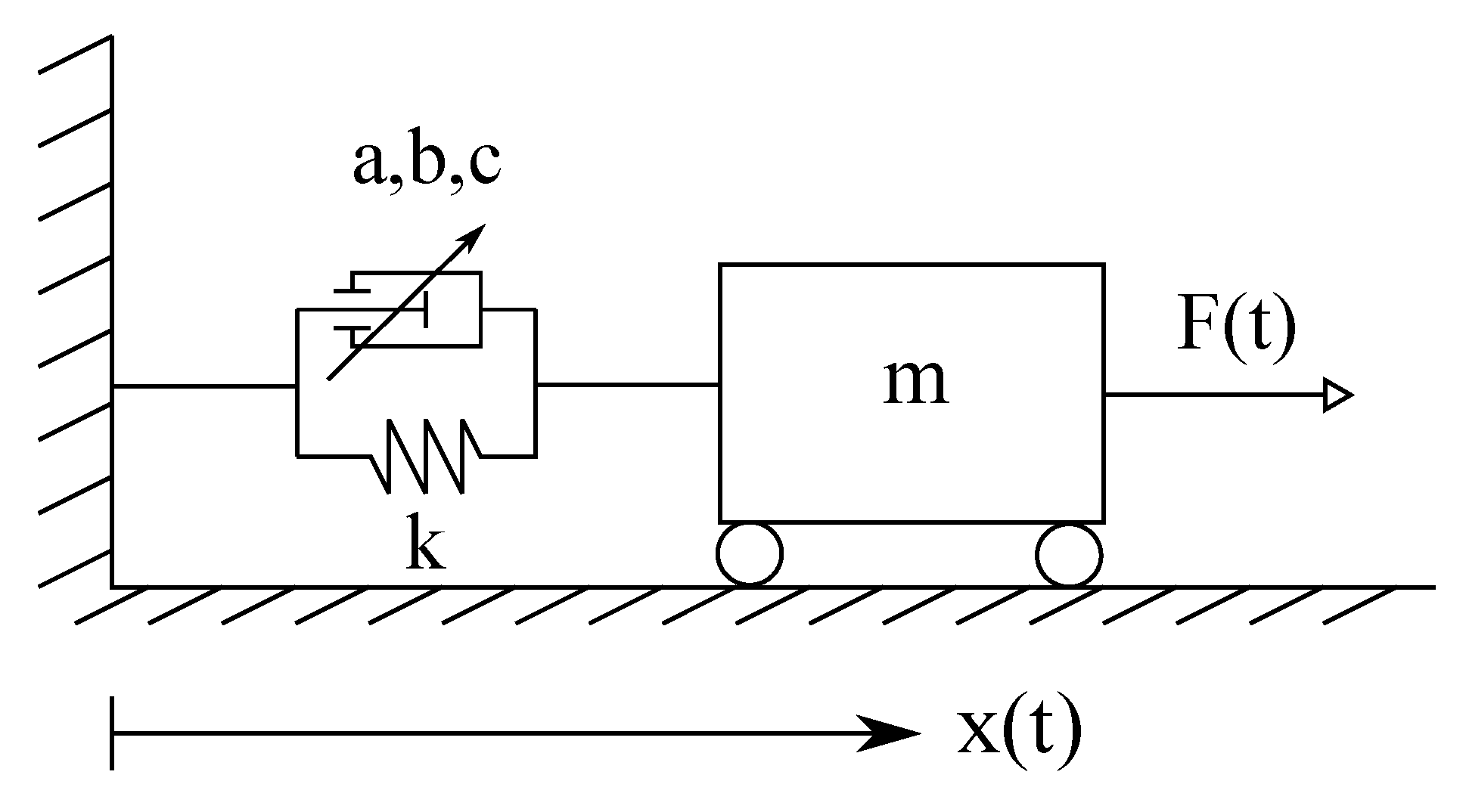
In this subsection, the demonstrative example considered as a case study is described. To this end, consider the mechanical system represented in Figure 2.
The mechanical system considered as a demonstrative example is a nonlinear oscillator with one degree of freedom indicated with , where x represents the displacement of the point mass. In Figure 2, m is the mass of the mechanical system, k represents the stiffness of the linear spring, whereas a, b, and c denote the constant coefficients of the nonlinear damper. The mechanical oscillator is connected to a nonlinear dashpot device based on the generalized Van der Pol damping model [86]. The force generated by the nonlinear damper is denoted with and is given by:
The nonlinear device shown in Figure 2 is based on the generalized Van der Pol damping model described by the force law given in Equation (25). Therefore, this component alternatively provides and drains mechanical energy from the nonlinear oscillator leading to a limit cycle in the system dynamical behavior. By using the analytical methods of classical mechanics, the nonlinear equation of motion of the mechanical oscillator can be readily written as follows:
where is the inertia force, represents the elastic force, and denotes a control force associated with a control actuator collocated on the mechanical oscillator. In this way, one can explicitly rewrite the system equation of motion as:
In particular, two general cases are considered, namely a feedforward controller described by the control action and a feedback controller described by the control action . In the case of a pure open-loop controller, the control action is an arbitrary function of time. In the case of a pure closed-loop controller, on the other hand, a simple linear structure is assumed for the control action given by:
where and are constant parameters defining the linear structure of the feedback controller, which can be groped in a two-dimensional parameter vector as follows:
Therefore, the feedback controller considered in this demonstrative example is based on the proportional-derivative control scheme. In the dynamical simulations, the following set of initial conditions is assumed for the nonlinear oscillator:
where represents the initial displacement of the particle and identifies the initial velocity of the point mass. In particular, a nonzero initial displacement and a zero initial velocity are selected for the nonlinear oscillator in order to set the initial configuration of the nonlinear system outside the region of the limit cycle that appear in the state-space diagram. Consequently, when there is no control action applied to the dynamical system, its spontaneous evolution is towards the limit cycle. The numerical data employed for performing the dynamical simulations are reported in Table 1.
Furthermore, in the numerical solution of the dynamic equation that describes the motion of the nonlinear oscillator, the dynamical simulations are performed considering a time interval equal to and a time step equal to . The numerical integration scheme employed for the numerical solution of the dynamic equation is the well-known fourth-order Adams–Bashforth method that represents a classical multistep explicit numerical integration algorithm.
3.2. Development of an Open-Loop Optimal Controller
In this subsection, the development of an optimal controller based on a feedforward control strategy is carried out for the nonlinear oscillator used as a demonstrative example employing the adjoint-based control optimization method. To this end, one can define a state vector for the mechanical oscillator given by:
By doing so, in the case of the design of an optimal open-loop controller, the equations of motion and the initial conditions can be represented in the state-space as follows:
where denotes the system state function and identifies the vector of initial conditions that are respectively defined in the case of an open-loop control action as follows:
In the case of an open-loop control architecture, the sensitivity matrices and can be readily calculated by evaluating the Jacobian matrices of the system state function as follows:
where and denote respectively the state matrix and the input influence matrix obtained by linearizing the system state function around the current system state and the current open-loop control force . The open-loop controller is a feedforward control scheme. The goal of the feedforward control action is to reduce the magnitude of the mechanical vibrations of the nonlinear oscillator without using an excessive amount of external energy associated with the control actuator. For this purpose, the terminal cost function h and the current cost function g can be simply constructed employing the following quadratic forms:
where , , and are diagonal matrices that define the weights of the terminal cost function h and the structure of the current cost function g. The numerical data used for the entries of the weight matrices necessary for the design of the optimal feedforward controller are , , and . Considering the analytical definitions of the terminal cost function h and of the current cost function g, one can readily determine the sensitivity vectors , , and associated with the feedforward controller as follows:
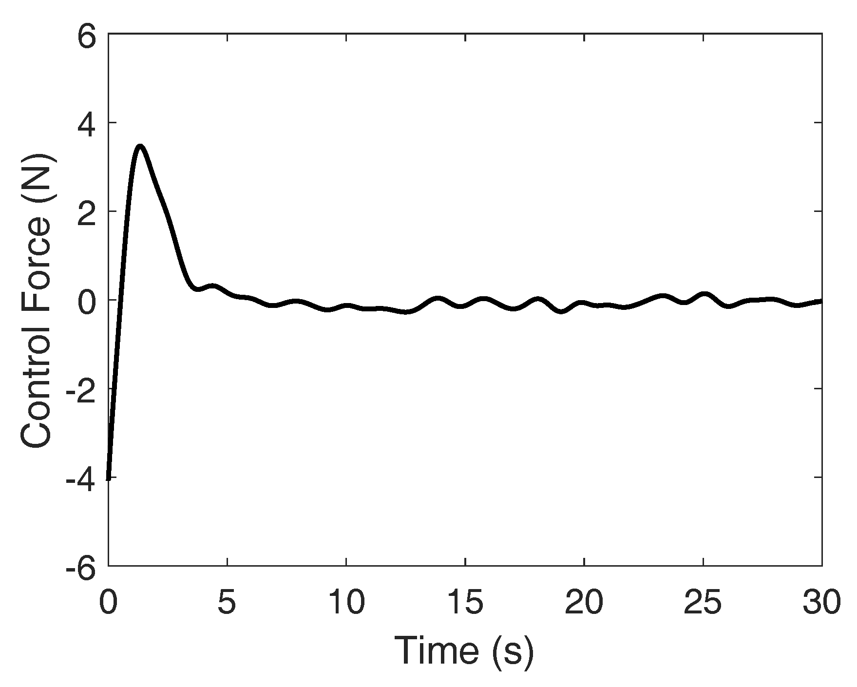
where is the perturbation vector of the terminal cost function h referred to the system state , is the perturbation vector of the current cost function g referred to the system state , and is the perturbation vector of the current cost function g referred to the open-loop control vector . Employing the sensitivity matrices and vectors defined before, the adjoint equations for the optimal design of a feedforward controller are analytically implemented and numerically solved by using a computer program developed in MATLAB (R2013a version). The initial guess for the feedforward control action used in the control optimization algorithm based on the adjoint approach is . Figure 3 shows the time law of the optimal feedforward control force resulting from the iterative numerical solution of the adjoint equations.
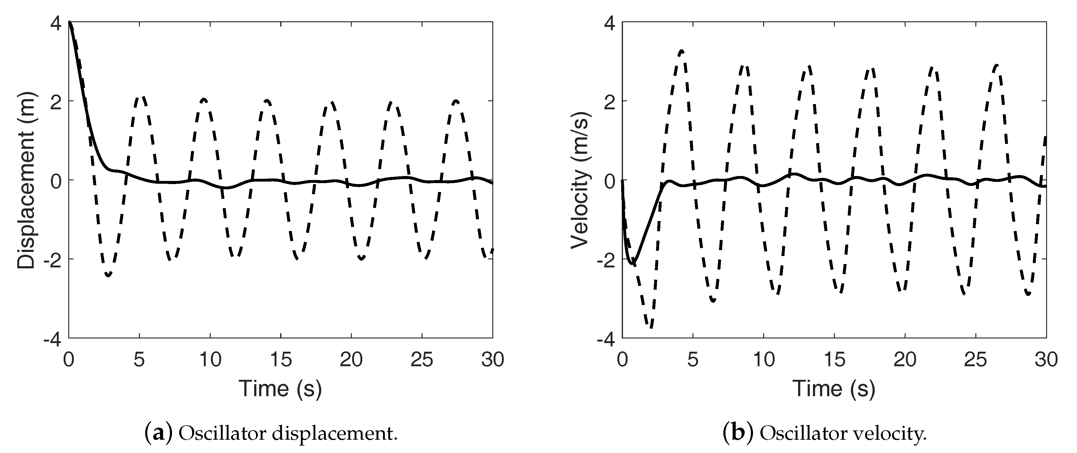
Figure 4a,b respectively show the displacement and velocity time histories relative to the mechanical oscillator used for testing the performance of the feedforward control action.
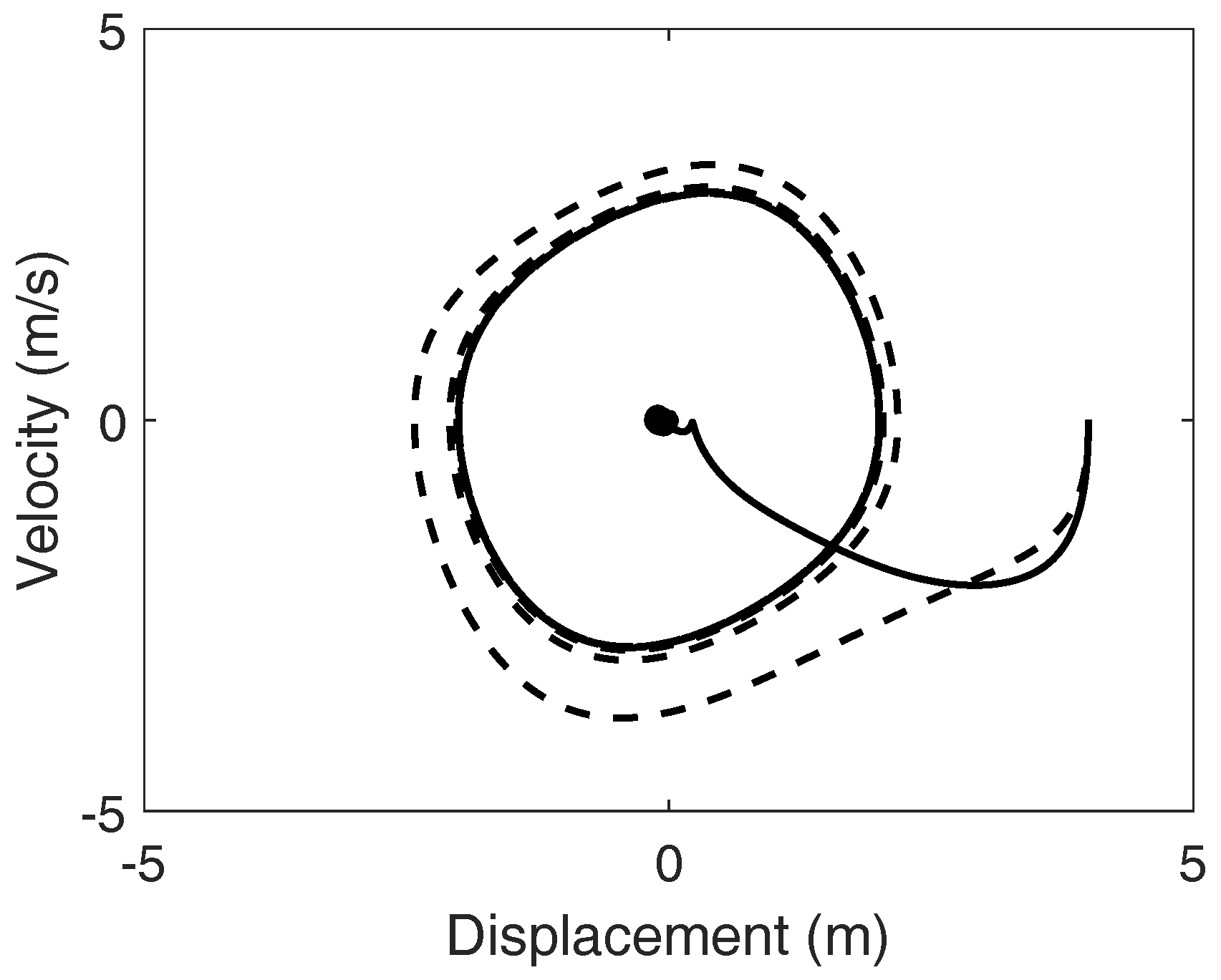
In Figure 4a,b, the dashed lines represent the time responses of the nonlinear oscillator when the control action is absent, whereas the solid lines represent the time responses of the mechanical oscillator when the optimal feedforward controller is active. The state-space representation of the dynamic evolution of the mechanical oscillator subjected to the action of the open-loop controller is shown in Figure 5.
In Figure 5, the dashed line represents the time response of the nonlinear oscillator when the open-loop control action is absent, whereas the solid line represents the time response of the mechanical oscillator when the optimal open-loop controller is active. As shown in Figure 4 and Figure 5, the feedforward control action represented in Figure 3 leads to a substantial attenuation of the mechanical vibrations of the nonlinear oscillator. In order to quantify the reduction of the mechanical vibrations, the Root-Mean-Square (RMS) deviations of the dynamical responses from the zero reference trajectory are computed with and without the action of the feedforward controller and the numerical results obtained are reported in Table 2.
Table 2 shows that the optimal open-loop control action obtained by using the control optimization procedure based on the adjoint approach effectively yields the desired vibration suppression.
3.3. Development of a Closed-Loop Optimal Controller
In this subsection, the development of an optimal controller based on a feedback control strategy is performed for the nonlinear oscillator used as a demonstrative example employing the adjoint-based parameter optimization method. For this purpose, one can define a state vector for the mechanical oscillator given by:
By doing so, in the case of the design of an optimal closed-loop controller, the equations of motion and the initial conditions can be rewritten in the state-space as follows:
where identifies the system state function and denotes the vector of initial conditions that are respectively defined in the case of a closed-loop control action as follows:
In the case of a closed-loop control architecture, the sensitivity matrices and can be easily derived by evaluating the Jacobian matrices of the system state function as follows:
where and indicate respectively the state matrix and the input influence matrix obtained by linearizing the system state function around the current system state and the current parameter vector that defines the structure of the closed-loop controller. The closed-loop controller is a feedback control scheme. The objective of the feedback control action is to reduce the entity of the mechanical vibrations of the nonlinear oscillator without using a large amount of external energy associated with the control actuator. To this end, the terminal cost function h and the current cost function g can be readily defined employing the following quadratic forms:
where , , and are diagonal matrices that describe the structure of the terminal cost function h and the weights of the current cost function g. The numerical data used for the entries of the weight matrices necessary for the design of the optimal feedback controller are , , and . Assuming the mathematical definitions of the terminal cost function h and of the current cost function g, one can readily determine the sensitivity vectors , , and associated with the feedback controller as follows:
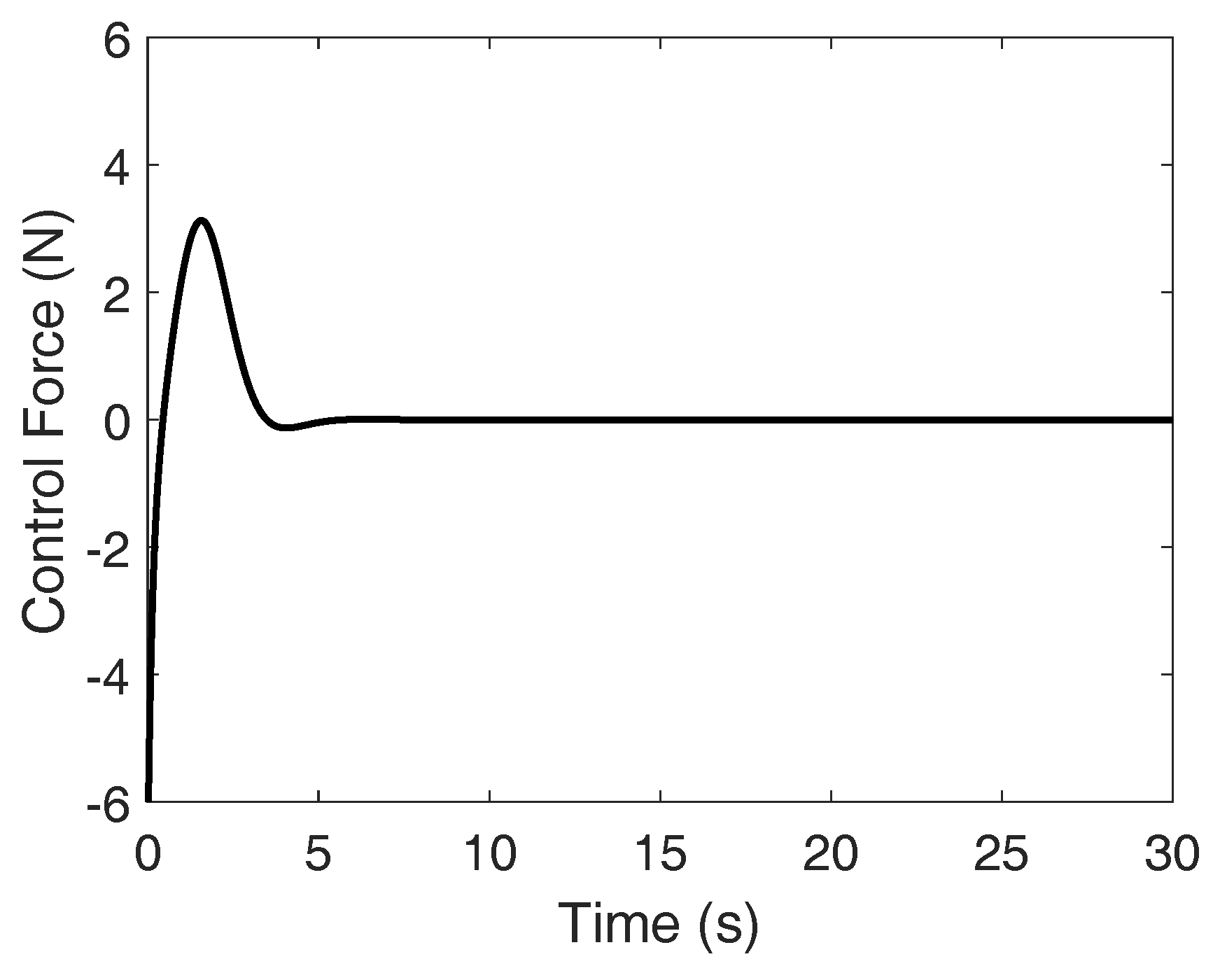
where is the perturbation vector of the terminal cost function h referred to the system state , is the perturbation vector of the current cost function g referred to the system state , and is the perturbation vector of the current cost function g referred to the parameter vector that defines the structure of the closed-loop controller. By using the sensitivity matrices and vector described above, the adjoint equations for the optimal design of a feedback controller are analytically implemented and numerically solved employing a computer program developed in MATLAB. The initial guess for the feedback control parameters used in the parameter optimization algorithm based on the adjoint approach are and . Figure 6 shows the time law of the optimal feedback control force resulting from the iterative numerical solution of the adjoint equations.
The optimal feedback controller represented in Figure 6 corresponds to the following optimal vector of control parameters obtained by means of the numerical implementation of the parameter optimization procedure based on the adjoint approach:
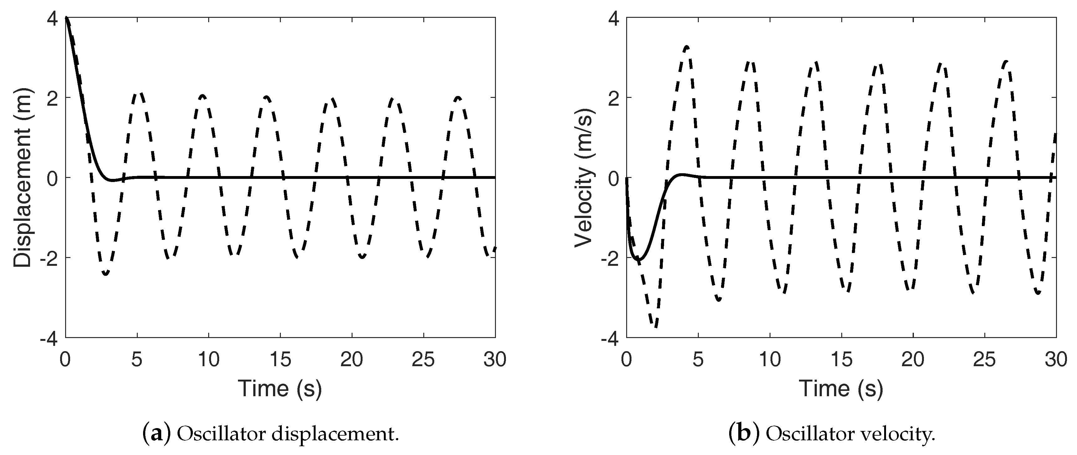
Figure 7a,b respectively show the displacement and velocity time histories relative to the mechanical oscillator used for testing the performance of the feedback control action.
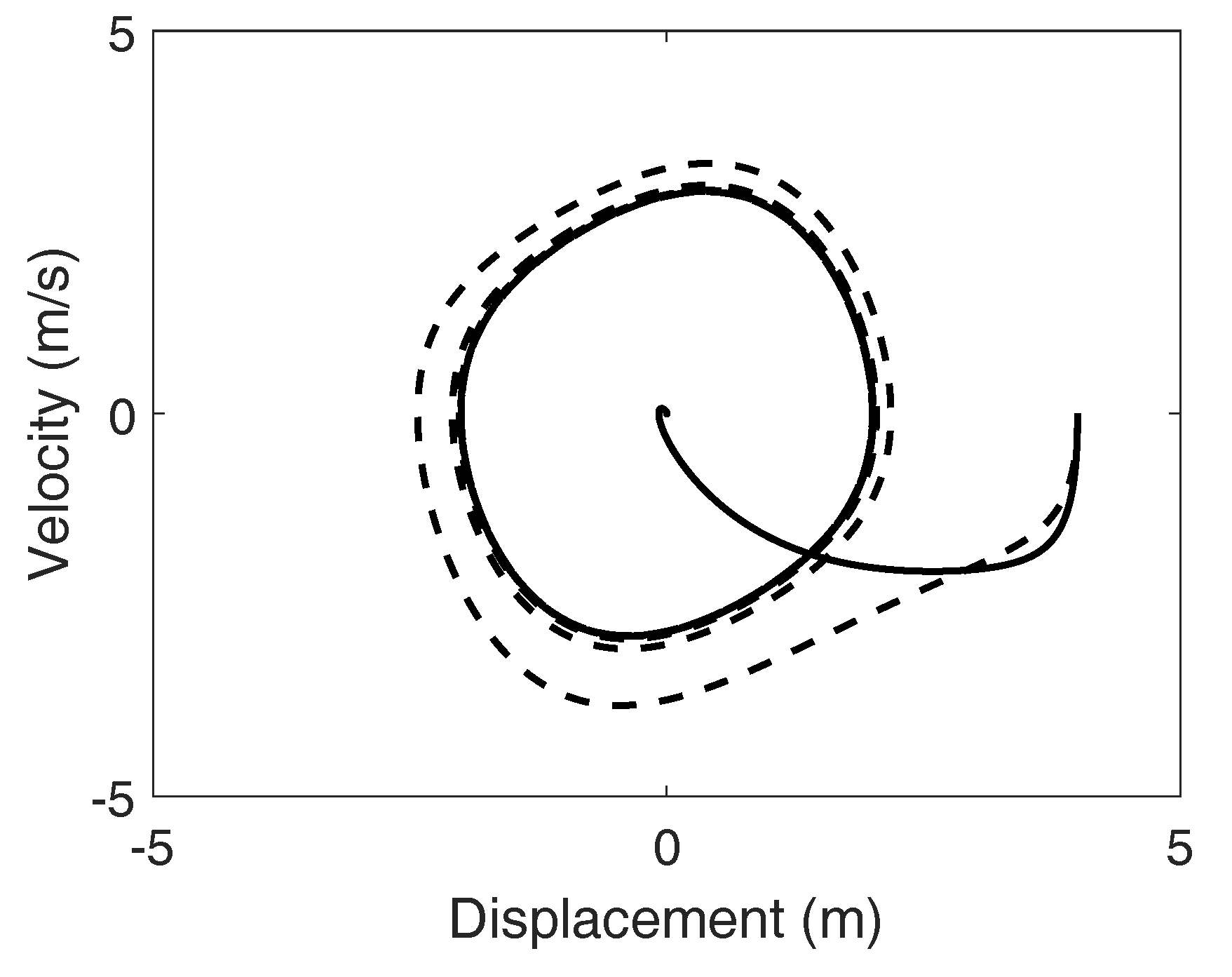
In Figure 7a,b, the dashed lines represent the time responses of the nonlinear oscillator when the control action is absent, whereas the solid lines represent the time responses of the mechanical oscillator when the optimal feedback controller is active. The state-space representation of the dynamic evolution of the mechanical oscillator subjected to the action of the closed-loop controller is shown in Figure 8.
In Figure 8, the dashed line represents the time response of the nonlinear oscillator when the closed-loop control action is absent, whereas the solid line represents the time response of the mechanical oscillator when the optimal closed-loop controller is active. As shown in Figure 7 and Figure 8, the feedback control action represented in Figure 6 leads to a considerable mitigation of the mechanical vibrations of the nonlinear oscillator. In order to quantify the reduction of the mechanical vibrations, the Root-Mean-Square (RMS) deviations of the dynamical responses from the zero reference trajectory are computed with and without the action of the feedback controller and the numerical results obtained are reported in Table 3.
Table 3 shows that the optimal closed-loop control action obtained by using the parameter optimization procedure based on the adjoint approach effectively produces the requested vibration attenuation.
4. Conclusions
The research of the authors is mainly focused on the development and the improvement of analytical methods and computational procedures for the nonlinear dynamic analysis of mechanical systems, for performing the experimental parameter identification of structural systems, and for the design of effective control strategies applicable to multibody systems [87,88,89,90]. For this purpose, the relationship between three different disciplines are exploited, namely the theory of nonlinear control, the numerical methods of applied system identification, and the analytical techniques of multibody system dynamics [91,92,93,94,95].
This work represents a study on the analytical derivation and the computer implementation of the adjoint method. The adjoint method can be effectively employed for constructing optimal control actions suitable for solving the regulation and tracking problems of a large class of nonlinear dynamical systems. In particular, the numerical solution of the nonlinear control problem addressed in this investigation is focused on two adjoint-based control methodologies. To this end, the iterative adjoint-based control algorithms discussed in this paper lead to the development of a nonlinear control optimization procedure and to the construction of a nonlinear parameter optimization procedure. The analytical derivation and the numerical implementation of the adjoint-based computational algorithms are illustrated in detail in this work. Furthermore, a demonstrative example is used in this paper for proving the effectiveness of the proposed method employing numerical experiments. For this purpose, the vibration control problem of the nonlinear oscillations of a mechanical system characterized by a generalized Van der Pol damping model is considered. The numerical results presented in the paper show that both the optimal feedforward and feedback controllers designed employing the proposed adjoint-based approach lead to a large reduction of the mechanical vibrations of the nonlinear oscillator that serves as a simple illustrative example.
In the field of nonlinear control, several complex algorithms have been developed in the recent years such as, for example, the methods based on the State-Dependent Riccati Equation (SDRE), the feedback linearization method, the sliding mode control approach, and nonlinear control methods based on the control-Lyapunov function. In general, the design of a nonlinear controller is a challenging task that may require the use of an iterative procedure, which cannot be directly implemented in real-time. This is also the case of the adjoint method developed in this investigation. However, for all the nonlinear control methods mentioned before, the underlying idea is that the development of a given control law can be performed offline by means of dynamical simulations. Subsequently, the control strategy developed employing extensive dynamical simulations can be implemented and tested online in a particular engineering application using an experimental test rig. By doing so, the computational complexity of the selected control strategy does not represent an issue because this calculation is performed only in advance in a virtual environment, which allows also to test the robustness and the effectiveness of the nonlinear control design. This concept is well-known in the control engineering community and represents one of the fundamental motivations behind the development of this investigation. Therefore, the nonlinear control method proposed in this paper is effectively applicable for solving actual engineering problems.
An important consideration that is worth emphasizing herein is the focus on the combined use of a feedforward control law with a feedback control strategy. This concept is another key idea commonly used in the control engineering community for the development of nonlinear controllers. Following this approach, an open-loop controller is at first designed employing a nonlinear dynamical model of a mechanical system that is the object of the control problem. Afterward, a closed-loop controller is designed in order to cope with the uncertainties of the model, the unavoidable presence of noise, and the incomplete measurement information on the state of the dynamical system. This approach represents a robust control paradigm that is widely accepted and used for nonlinear control applications and this paper is based on this background idea. Furthermore, this investigation proposes a complex control algorithm that can be tested on simple dynamical systems in order to allow other researchers to reproduce the numerical results proposed in the paper and compare the performance of the adjoint-based approach with the effectiveness of other viable control strategies.
An additional important aspect of the optimal control problem associated with nonlinear mechanical systems concerns the process noise and the measurement uncertainties arising from the interaction between the mechanical system and the external world modelled as a stochastic environment. This challenging problem directly involves the use of a state estimator referred to as an observer. This complex scenario can be handled with the methodology proposed in the paper in conjunction with the mathematical tools of the modern optimal estimation and control theory. To this end, the adjoint-based procedure can be effectively used to derive optimal control actions for a nominal model of the mechanical system under examination. Subsequently, the nonlinear behavior of the mechanical system can be linearized around the operational trajectory obtained from the control action applied to the nominal system. Thus, an optimal controller together with an optimal observer can be designed using the linearized dynamical model. For this purpose, several control and estimation algorithms can be employed considering the linearized dynamical model. For example, the Linear-Quadratic-Gaussian (LQG) control and estimation method based on the Kalman filtering technique can be employed in order to effectively accomplish this task. By doing so, an optimal compensation controller can be obtained in order to adjust the difference in the dynamical behavior of the nominal dynamic model with respect to the actual mechanical system on which the controller is implemented. Following this alternative approach suitable for handling practical engineering problems, the combination of the nominal controller designed employing the adjoint-based procedures with the compensation controller obtained using the LQG technique can lead to a robust control strategy capable of coping with the power limit in the actuators, the presence of noise in the system process and in the measurements, and the lack of information on the system state.
This paper represents a step further in a wider research plan devised by the authors and focused on the use of the optimization approach for solving the nonlinear control problem in the case of the dynamic behavior of mechanical systems. Future research efforts will be devoted to the development of effective adjoint-based nonlinear control actions for differential-algebraic dynamical systems, such as the multibody mechanical systems, by using advanced analytical techniques tested employing numerical simulations. Moreover, the experimental validation of the numerical results obtained for attenuating the nonlinear mechanical vibrations of complex dynamical systems commonly employed in engineering applications such as machines and structures will be performed in future investigations.
Author Contributions
This research paper was principally developed by the first author (Carmine Maria Pappalardo). The detailed review carried out by the second author (Domenico Guida) considerably improved the quality of the work.
Funding
This research received no external funding.
Conflicts of Interest
The authors declare no conflict of interest.
References
- Udwadia, F.E.; Kalaba, R.E. Analytical Dynamics: A New Approach; Cambridge University Press: New York, NY, USA, 2007. [Google Scholar]
- Juang, J.N.; Phan, M.Q. Identification and Control of Mechanical Systems; Cambridge University Press: New York, NY, USA, 2001. [Google Scholar]
- Zhai, Y.; Liu, L.; Lu, W.; Li, Y.; Yang, S.; Villecco, F. The Application of Disturbance Observer to Propulsion Control of Sub-mini Underwater Robot. In Proceedings of the ICCSA 2010 International Conference on Computational Science and Its Applications, Fukuoka, Japan, 23–26 March 2010; Lecture Notes in Computer Science. Springer: Berlin, Germany, 2010; pp. 590–598. [Google Scholar]
- Villecco, F.; Pellegrino, A. Entropic Measure of Epistemic Uncertainties in Multibody System Models by Axiomatic Design. Entropy 2017, 19, 291. [Google Scholar] [CrossRef]
- Villecco, F.; Pellegrino, A. Evaluation of Uncertainties in the Design Process of Complex Mechanical Systems. Entropy 2017, 19, 475. [Google Scholar] [CrossRef]
- Gao, Y.; Villecco, F.; Li, M.; Song, W. Multi-Scale Permutation Entropy Based on Improved LMD and HMM for Rolling Bearing Diagnosis. Entropy 2017, 19, 176. [Google Scholar] [CrossRef]
- Pappalardo, M.; Villecco, F. Max-Ent in fast belief fusion. In Proceedings of the International Conference Differential Geometry, Dynamical Systems, Bucharest, Romania, 5–7 October 2007; Geometry Balkan Press, Univ Politehnica Bucharest: Bucharest, Romania, 2008; pp. 154–162. [Google Scholar]
- Zhang, Y.; Li, Z.; Gao, J.; Hong, J.; Villecco, F.; Li, Y. A method for designing assembly tolerance networks of mechanical assemblies. Math. Probl. Eng. 2012, 2012, 513958. [Google Scholar] [CrossRef]
- Sansone, F.; Picerno, P.; Mencherini, T.; Villecco, F.; D’Ursi, A.M.; Aquino, R.P.; Lauro, M.R. Flavonoid Microparticles by Spray-Drying: Influence of Enhancers of the Dissolution Rate on Properties and Stability. J. Food Eng. 2001, 103, 188–196. [Google Scholar] [CrossRef]
- Pellegrino, A.; Villecco, F. Design Optimization of a Natural Gas Substation with Intensification of the Energy Cycle. Math. Probl. Eng. 2010, 2010, 294102. [Google Scholar] [CrossRef]
- Ghomshei, M.; Villecco, F.; Porkhial, S.; Pappalardo, M. Complexity in Energy Policy: A Fuzzy Logic Methodology. In Proceedings of the 6th International Conference on Fuzzy Systems and Knowledge Discovery, Tianjin, China, 14–16 August 2009; IEEE: Los Alamitos, CA, USA, 2009; Volume 7, pp. 128–131. [Google Scholar]
- Ghomshei, M.; Villecco, F. Energy Metrics and Sustainability. In Proceedings of the International Conference on Computational Science and Its Applications, Seoul, Korea, 29 June–2 July 2009; Lecture Notes in Computer Science. Springer: Berlin, Germany, 2009; pp. 693–698. [Google Scholar]
- Cattani, C.; Mercorelli, P.; Villecco, F.; Harbusch, K. A theoretical multiscale analysis of electrical field for fuel cells stack structures. In Proceedings of the International Conference on Computational Science and Its Applications, Glasgow, UK, 8–11 May 2006; Springer: Berlin/Heidelberg, Germany, 2006; pp. 857–864. [Google Scholar]
- Formato, A.; Ianniello, D.; Villecco, F.; Lenza, T.L.L.; Guida, D. Design Optimization of the Plough Working Surface by Computerized Mathematical Model. Emir. J. Food Agric. 2017, 29, 36–44. [Google Scholar] [CrossRef]
- Sena, P.; D’Amore, M.; Pappalardo, M.; Pellegrino, A.; Fiorentino, A.; Villecco, F. Studying the Influence of Cognitive Load on Driver’s Performances by a Fuzzy Analysis of Lane Keeping in a Drive Simulation. IFAC Proc. Vol. 2013, 46, 151–156. [Google Scholar] [CrossRef]
- Sena, P.; Attianese, P.; Pappalardo, M.; Villecco, F. FIDELITY: Fuzzy Inferential Diagnostic Engine for on-LIne supporT to phYsicians. In Proceedings of the 4th International Conference on the Development of Biomedical Engineering, Ho Chi Minh City, Vietnam, 8–10 January 2012; IFMBE Proceedings. Springer: Berlin, Germany, 2013; pp. 396–400. [Google Scholar]
- Sena, P.; Attianese, P.; Carbone, F.; Pellegrino, A.; Pinto, A.; Villecco, F. A Fuzzy Model to Interpret Data of Drive Performances from Patients with Sleep Deprivation. Comput. Math. Methods Med. 2012, 2012, 868410. [Google Scholar] [CrossRef] [PubMed]
- Khalil, H.K. Nonlinear Systems, 3rd ed.; Prentice Hall: Upper Saddle River, NJ, USA, 2001. [Google Scholar]
- Strano, S.; Terzo, M. Actuator Dynamics Compensation for Real-time Hybrid Simulation: An Adaptive Approach by means of a Nonlinear Estimator. Nonlinear Dyn. 2016, 85, 2353–2368. [Google Scholar] [CrossRef]
- Strano, S.; Terzo, M. Accurate State Estimation for a Hydraulic Actuator via a SDRE Nonlinear Filter. Mech. Syst. Signal Process. 2016, 75, 576–588. [Google Scholar] [CrossRef]
- Russo, R.; Strano, S.; Terzo, M. Enhancement of Vehicle Dynamics via an Innovative Magnetorheological Fluid Limited Slip Differential. Mech. Syst. Signal Process. 2016, 70, 1193–1208. [Google Scholar] [CrossRef]
- Strano, S.; Terzo, M. A SDRE-based Tracking Control for a Hydraulic Actuation System. Mech. Syst. Signal Process. 2015, 60, 715–726. [Google Scholar] [CrossRef]
- Sharifzadeh, M.; Farnam, A.; Senatore, A.; Timpone, F.; Akbari, A. Delay-Dependent Criteria for Robust Dynamic Stability Control of Articulated Vehicles. In Proceedings of the International Conference on Robotics in Alpe-Adria Danube Region, Torino, Italy, 21–23 June 2017; pp. 424–432. [Google Scholar]
- Sharifzadeh, M.; Timpone, F.; Farnam, A.; Senatore, A.; Akbari, A. Tyre-road Adherence Conditions Estimation for Intelligent Vehicle Safety Applications. In Advances in Italian Mechanism Science, Mechanisms and Machine Science; Springer: Cham, Switzerlane, 2017; Volume 47, pp. 389–398. [Google Scholar]
- Roman, R.C.; Radac, M.B.; Precup, R.E.; Petriu, E.M. Virtual Reference Feedback Tuning of Model-Free Control Algorithms for Servo Systems. Machines 2017, 5, 25. [Google Scholar] [CrossRef]
- Precup, R.E.; David, R.C.; Szedlak-Stinean, A.I.; Petriu, E.M.; Dragan, F. An Easily Understandable Grey Wolf Optimizer and Its Application to Fuzzy Controller Tuning. Algorithms 2017, 10, 68. [Google Scholar] [CrossRef]
- Radac, M.B.; Precup, R.E. Data-Driven Model-Free Slip Control of Anti-Lock Braking Systems using Reinforcement Q-Learning. Neurocomputing 2018, 275, 317–329. [Google Scholar] [CrossRef]
- Radac, M.B.; Precup, R.E.; Roman, R.C. Data-Driven Model Reference Control of MIMO Vertical Tank Systems with Model-Free VRFT and Q-Learning. ISA Trans. 2018, 73, 22–30. [Google Scholar] [CrossRef] [PubMed]
- Pozna, C.; Precup, R.E. On a Translated Frame-Based Approach to Geometric Modeling of Robots. Robot. Auton. Syst. 2017, 91, 49–58. [Google Scholar] [CrossRef]
- Patel, M.; Orzechowski, G.; Tian, Q.; Shabana, A.A. A New Multibody System Approach for Tire Modeling using ANCF Finite Elements. Proc. Inst. Mech. Eng. Part K J. Multibody 2016, 230, 69–84. [Google Scholar] [CrossRef]
- Barbagallo, R.; Sequenzia, G.; Cammarata, A.; Oliveri, S.M.; Fatuzzo, G. Redesign and Multibody Simulation of a Motorcycle Rear Suspension with Eccentric Mechanism. Int. J. Interact. Des. Manuf. 2017, 1–8. [Google Scholar] [CrossRef]
- Marques, F.; Souto, A.P.; Flores, P. On the Constraints Violation in Forward Dynamics of Multibody Systems. Multibody Syst. Dyn. 2017, 39, 385–419. [Google Scholar] [CrossRef]
- Cammarata, A.; Calio, I.; Greco, A.; Lacagnina, M.; Fichera, G. Dynamic Stiffness Model of Spherical Parallel Robots. Sound Vib. 2016, 384, 312–324. [Google Scholar] [CrossRef]
- Cammarata, A. Unified Formulation for the Stiffness Analysis of Spatial Mechanisms. Mech. Mach. Theory 2016, 105, 272–284. [Google Scholar] [CrossRef]
- Cammarata, A.; Angeles, J.; Sinatra, R. The Dynamics of Parallel Schonflies Motion Generators: The Case of a Two-limb System. Proc. Inst. Mech. Eng. I J. Syst. 2009, 223, 29–52. [Google Scholar] [CrossRef]
- Kulkarni, S.; Pappalardo, C.M.; Shabana, A.A. Pantograph/Catenary Contact Formulations. J. Vib. Acoust. 2017, 139, 011010. [Google Scholar] [CrossRef]
- Pappalardo, C.M.; Patel, M.D.; Tinsley, B.; Shabana, A.A. Contact Force Control in Multibody Pantograph/Catenary Systems. Proc. Inst. Mech. Eng. Part K J. Multibody Dyn. 2016, 230, 307–328. [Google Scholar] [CrossRef]
- De Simone, M.C.; Guida, D. On the Development of a Low Cost Device for Retrofitting Tracked Vehicles for Autonomous Navigation. In Proceedings of the AIMETA 2017—XXIII Conference of The Italian Association of Theoretical and Applied Mechanics, Salerno, Italy, 4–7 September 2017. [Google Scholar]
- Ruggiero, A.; Affatato, S.; Merola, M.; De Simone, M.C. FEM Analysis of Metal on UHMWPE Total Hip Prosthesis During Normal Walking Cycle. In Proceedings of the AIMETA 2017—XXIII Conference of The Italian Association of Theoretical and Applied Mechanics, Salerno, Italy, 4–7 September 2017. [Google Scholar]
- De Simone, M.C.; Rivera, Z.B.; Guida, D. Finite Element Analysis on Squeal-Noise in Railway Applications. FME Trans. 2018, 46, 93–100. [Google Scholar]
- De Simone, M.C.; Russo, S.; Rivera, Z.B.; Guida, D. Multibody model of a UAV in presence of wind fields. In Proceedings of the ICCAIRO 2017 International Conference on Control, Artificial Intelligence, Robotics and Optimization, Prague, Czech Republic, 20–22 May 2017. [Google Scholar]
- Pappalardo, C.M.; Wallin, M.; Shabana, A.A. A New ANCF/CRBF Fully Parametrized Plate Finite Element. J. Comput. Nonlinear Dyn. 2017, 12, 031008. [Google Scholar] [CrossRef]
- Pappalardo, C.M.; Yu, Z.; Zhang, X.; Shabana, A.A. Rational ANCF Thin Plate Finite Element. J. Comput. Nonlinear Dyn. 2016, 11, 051009. [Google Scholar] [CrossRef]
- Quatrano, A.; De Simone, M.C.; Rivera, Z.B.; Guida, D. Development and implementation of a control system for a retrofitted CNC machine by using Arduino. FME Trans. 2017, 45, 565–571. [Google Scholar] [CrossRef]
- Concilio, A.; De Simone, M.C.; Rivera, Z.B.; Guida, D. A new semi-active suspension system for racing vehicles. FME Trans. 2017, 45, 578–584. [Google Scholar] [CrossRef]
- Pappalardo, C.M.; Guida, D. On the Lagrange Multipliers of the Intrinsic Constraint Equations of Rigid Multibody Mechanical Systems. Arch. Appl. Mech. 2018, 88, 419–451. [Google Scholar] [CrossRef]
- Pappalardo, C.M.; Guida, D. On the Use of Two-dimensional Euler Parameters for the Dynamic Simulation of Planar Rigid Multibody Systems. Arch. Appl. Mech. 2017, 87, 1647–1665. [Google Scholar] [CrossRef]
- Guida, D.; Pappalardo, C.M. Forward and Inverse Dynamics of Nonholonomic Mechanical Systems. Meccanica 2014, 49, 1547–1559. [Google Scholar] [CrossRef]
- Pappalardo, C.M. A Natural Absolute Coordinate Formulation for the Kinematic and Dynamic Analysis of Rigid Multibody Systems. Nonlinear Dyn. 2015, 81, 1841–1869. [Google Scholar] [CrossRef]
- Pappalardo, C.M.; Guida, D. Dynamic Analysis of Planar Rigid Multibody Systems modelled using Natural Absolute Coordinates. Appl. Comput. Mech. 2018. accepted. [Google Scholar]
- Pappalardo, C.M. Modelling Rigid Multibody Systems using Natural Absolute Coordinates. J. Mech. Eng. Ind. Des. 2014, 3, 24–38. [Google Scholar]
- Lan, P.; Shabana, A.A. Rational Finite Elements and Flexible Body Dynamics. J. Vib. Acoust. 2010, 132, 041007. [Google Scholar] [CrossRef]
- Liu, C.; Tian, Q.; Hu, H.; Garcia-Vallejo, D. Simple Formulations of Imposing Moments and Evaluating Joint Reaction Forces for Rigid-flexible Multibody Systems. Nonlinear Dyn. 2012, 69, 127–147. [Google Scholar] [CrossRef]
- Tian, Q.; Chen, L.P.; Zhang, Y.Q.; Yang, J. An Efficient Hybrid Method for Multibody Dynamics Simulation based on Absolute Nodal Coordinate Formulation. J. Comput. Nonlinear Dyn. 2009, 4, 021009. [Google Scholar] [CrossRef]
- Hu, W.; Tian, Q.; Hu, H. Dynamic Simulation of Liquid-filled Flexible Multibody Systems via Absolute Nodal Coordinate Formulation and SPH Method. Nonlinear Dyn. 2014, 75, 653–671. [Google Scholar] [CrossRef]
- Liu, C.; Tian, Q.; Hu, H. Dynamics of a Large Scale Rigid–flexible Multibody System Composed of Composite Laminated Plates. Multibody Syst. Dyn. 2011, 26, 283–305. [Google Scholar] [CrossRef]
- Pappalardo, C.M.; Wang, T.; Shabana, A.A. On the Formulation of the Planar ANCF Triangular Finite Elements. Nonlinear Dyn. 2017, 89, 1019–1045. [Google Scholar] [CrossRef]
- Pappalardo, C.M.; Wang, T.; Shabana, A.A. Development of ANCF Tetrahedral Finite Elements for the Nonlinear Dynamics of Flexible Structures. Nonlinear Dyn. 2017, 89, 2905–2932. [Google Scholar] [CrossRef]
- Pappalardo, C.M.; Zhang, Z.; Shabana, A.A. Use of Independent Volume Parameters in the Development of New Large Displacement ANCF Triangular Plate/Shell Elements. Nonlinear Dyn. 2018, 91, 2171–2202. [Google Scholar] [CrossRef]
- Nachbagauer, K.; Oberpeilsteiner, S.; Sherif, K.; Steiner, W. The Use of the Adjoint Method for Solving Typical Optimization Problems in Multibody Dynamics. J. Comput. Nonlinear Dyn. 2015, 10, 061011. [Google Scholar] [CrossRef]
- Oberpeilsteiner, S.; Lauss, T.; Nachbagauer, K.; Steiner, W. Optimal Input Design for Multibody Systems by using an Extended Adjoint Approach. Multibody Syst. Dyn. 2017, 40, 43–54. [Google Scholar] [CrossRef] [PubMed]
- Udwadia, F.E.; Wanichanon, T. On General Nonlinear Constrained Mechanical Systems. Am. Inst. Math. Sci. 2013, 3, 425–443. [Google Scholar] [CrossRef]
- Schutte, A.; Udwadia, F. New Approach to the Modeling of Complex Multibody Dynamical Systems. J. Appl. Mech. 2011, 78, 021018. [Google Scholar] [CrossRef]
- Pennestrí, E.; Valentini, P.P.; De Falco, D. An Application of the Udwadia-Kalaba Dynamic Formulation to Flexible Multibody Systems. J. Frankl. Inst. 2010, 347, 173–194. [Google Scholar] [CrossRef]
- De Falco, D.; Pennestrí, E.; Vita, L. Investigation of the Influence of Pseudoinverse Matrix Calculations on Multibody Dynamics Simulations by means of the Udwadia-Kalaba Formulation. J. Aerospace Eng. 2009, 22, 365–372. [Google Scholar] [CrossRef]
- Luchini, P.; Bottaro, A. Adjoint Equations in Stability Analysis. Ann. Rev. Fluid Mech. 2014, 46, 1–30. [Google Scholar] [CrossRef]
- Luchini, P.; Bewley, T.R. Methods for the Solution of Very Large Flow-Control Problems that Bypass Open-Loop Model Reduction. Meccanica 2010, 55–16, 42. [Google Scholar]
- Kim, J.; Bewley, T.R. A Linear Systems Approach to Flow Control. Ann. Rev. Fluid Mech. 2007, 39, 383–417. [Google Scholar] [CrossRef]
- Bewley, T.R. Flow Control: New Challenges for a New Renaissance. Prog. Aerosp. Sci. 2001, 37, 21–58. [Google Scholar] [CrossRef]
- Giles, M.B.; Pierce, N.A. An Introduction to the Adjoint Approach to Design. Flow Turbulence Combust. 2000, 65, 393–415. [Google Scholar] [CrossRef]
- Luchini, P.; Giannetti, F.; Citro, V. Error Sensitivity to Refinement: A Criterion for Optimal Grid Adaptation. Theor. Comp. Fluid Dyn. 2017, 31, 595–605. [Google Scholar] [CrossRef]
- Citro, V.; Giannetti, F.; Brandt, L.; Luchini, P. Linear Three-Dimensional Global and Asymptotic Stability Analysis of Incompressible Open Cavity Flow. J. Fluid Mech. 2015, 768, 113–140. [Google Scholar] [CrossRef]
- Rigatos, G.; Siano, P.; Ghosh, T. A Nonlinear Optimal Control Approach to Stabilization of Business Cycles of Finance Agents. Comput. Econ. 2017, 1–21. [Google Scholar] [CrossRef]
- Rigatos, G.; Siano, P.; Abbaszadeh, M. Nonlinear H-Infinity Control for 4-DOF Underactuated Overhead Cranes. Trans. Inst. Meas. Control 2017, 40, 2364–2377. [Google Scholar] [CrossRef]
- Pappalardo, C.M.; Guida, D. Adjoint-based Optimization Procedure for Active Vibration Control of Nonlinear Mechanical Systems. J. Dyn. Syst. Meas. Control 2017, 139, 081010. [Google Scholar] [CrossRef]
- Guida, D.; Pappalardo, C.M. Control Design of an Active Suspension System for a Quarter-Car Model with Hysteresis. J. Vib. Eng. Technol. 2015, 3, 277–299. [Google Scholar]
- Vincent, T.L.; Grantham, J.W. Nonlinear and Optimal Control Systems; Wiley: New York, NY, USA, 1997. [Google Scholar]
- Betts, J.T. Practical Methods for Optimal Control and Estimation Using Nonlinear Programming, 2nd ed.; The Boeing Company: Seattle, MA, USA, 2010. [Google Scholar]
- Stengel, R.F. Optimal Control and Estimation; Dover: New York, NY, USA, 1986. [Google Scholar]
- Pappalardo, C.M.; Guida, D. Control of Nonlinear Vibrations using the Adjoint Method. Meccanica 2017, 52, 2503–2526. [Google Scholar] [CrossRef]
- Guida, D.; Pappalardo, C.M. A New Control Algorithm for Active Suspension Systems Featuring Hysteresis. FME Trans. 2013, 41, 285–290. [Google Scholar]
- Nise, N.S. Control System Engineering, 6th ed.; Wiley: New York, NY, USA, 2011. [Google Scholar]
- Lewis, F.L.; Vrabie, D.L.; Syrmos, V.L. Optimal Control, 3rd ed.; Wiley: New York, NY, USA, 2012. [Google Scholar]
- Kirk, D.E. Optimal Control Theory: An Introduction; Dover: Mineola, NY, USA, 2012. [Google Scholar]
- Bertsekas, D.P. Dynamic Programming and Optimal Control, Volume I and II; Athena Scientific: Belmont, MA, USA, 2005. [Google Scholar]
- Nayfeh, A.H.; Mook, D.T. Nonlinear Oscillations; Wiley: New York, NY, USA, 1995. [Google Scholar]
- De Simone, M.C.; Guida, D. Identification and Control of a Unmanned Ground Vehicle By using Arduino. UPB Sci. Bull. Ser. D 2018, 80, 141–154. [Google Scholar]
- De Simone, M.C.; Guida, D. Modal Coupling in Presence of Dry Friction. Machines 2018, 6, 8. [Google Scholar] [CrossRef]
- De Simone, M.C.; Guida, D. Dry Friction Influence on Structure Dynamics. In Proceedings of the COMPDYN 2015—5th ECCOMAS Thematic Conference on Computational Methods in Structural Dynamics and Earthquake Engineering, Crete, Greece, 25–27 May 2015; pp. 4483–4491. [Google Scholar]
- Ruggiero, A.; De Simone, M.C.; Russo, D.; Guida, D. Sound Pressure Measurement of Orchestral Instruments in the Concert Hall of a Public School. Int. J. Circuits Syst. Signal Process. 2016, 10, 75–81. [Google Scholar]
- Guida, D.; Nilvetti, F.; Pappalardo, C.M. Parameter Identification of a Two Degrees of Freedom Mechanical System. Int. J. Mech. 2009, 3, 23–30. [Google Scholar]
- Guida, D.; Pappalardo, C.M. Sommerfeld and Mass Parameter Identification of Lubricated Journal Bearing. WSEAS Trans. Appl. Theor. Mech. 2009, 4, 205–214. [Google Scholar]
- Pappalardo, C.M.; Guida, D. System Identification and Experimental Modal Analysis of a Frame Structure. Eng. Let. 2018, 26, 56–68. [Google Scholar]
- Guida, D.; Nilvetti, F.; Pappalardo, C.M. Instability Induced by Dry Friction. Int. J. Mech. 2009, 3, 44–51. [Google Scholar]
- Guida, D.; Nilvetti, F.; Pappalardo, C.M. Dry Friction Influence on Cart Pendulum Dynamics. Int. J. Mech. 2009, 3, 31–38. [Google Scholar]
Figure 1.
Adjoint iterative computational algorithm.

Figure 2.
Nonlinear mechanical oscillator.

Figure 3.
Optimal feedforward controller.

Figure 4.
Uncontrolled motion (dashed line) and feedforward controlled motion (solid line).

Figure 5.
Uncontrolled state-space trajectory (dashed line) and feedforward controlled state-space trajectory (solid line).
Figure 5.
Uncontrolled state-space trajectory (dashed line) and feedforward controlled state-space trajectory (solid line).

Figure 6.
Optimal feedback controller.

Figure 7.
Uncontrolled motion (dashed line) and feedback controlled motion (solid line).

Figure 8.
Uncontrolled state-space trajectory (dashed line) and feedback controlled state-space trajectory (solid line).
Figure 8.
Uncontrolled state-space trajectory (dashed line) and feedback controlled state-space trajectory (solid line).


Table 1.
Nonlinear oscillator numerical parameters.
| Description | Symbols | Data (Units) |
|---|---|---|
| System Mass | m | |
| Spring Stiffness | k | |
| Damper First Coefficient | a | |
| Damper Second Coefficient | b | |
| Damper Third Coefficient | c | |
| Initial Displacement | 4 (m) | |
| Initial Velocity |
Table 2.
Performance of the Optimal Feedforward Controller.
| Uncontrolled Motion RMS | Controlled Motion RMS | Relative Reduction | |
|---|---|---|---|
| Displacement | 1.5752 | 0.6681 | 57.59 % |
| Velocity | 2.0819 | 0.4525 | 78.25 % |
Table 3.
Performance of the Optimal Feedback Controller.
| Uncontrolled Motion RMS | Controlled Motion RMS | Relative Reduction | |
|---|---|---|---|
| Displacement | 1.5752 | 0.6525 | 58.58 % |
| Velocity | 2.0819 | 0.4752 | 77.16 % |
© 2018 by the authors. Licensee MDPI, Basel, Switzerland. This article is an open access article distributed under the terms and conditions of the Creative Commons Attribution (CC BY) license (http://creativecommons.org/licenses/by/4.0/).
Share and Cite
MDPI and ACS Style
Pappalardo, C.M.; Guida, D. Use of the Adjoint Method for Controlling the Mechanical Vibrations of Nonlinear Systems. Machines 2018, 6, 19. https://doi.org/10.3390/machines6020019
AMA Style
Pappalardo CM, Guida D. Use of the Adjoint Method for Controlling the Mechanical Vibrations of Nonlinear Systems. Machines. 2018; 6(2):19. https://doi.org/10.3390/machines6020019
Chicago/Turabian StylePappalardo, Carmine Maria, and Domenico Guida. 2018. "Use of the Adjoint Method for Controlling the Mechanical Vibrations of Nonlinear Systems" Machines 6, no. 2: 19. https://doi.org/10.3390/machines6020019
Note that from the first issue of 2016, this journal uses article numbers instead of page numbers. See further details here.