On the Evaluation of Errors in the Virtual Design of Mechanical Systems

Abstract

In this article, the information value is used in numeric analysis as both a method for data approximation and a measure of data equality among a set of values. To this end, a surface segmentation, based on a study for constructing a hierarchy for vectors clustering using certain similarity criteria, is presented. The technique is based on the analysis of vectors representing regions associated with given types of critical points. An approach based on the Max Entropy in Metric Space (MEMS) is introduced in the paper, in order to extract a cluster of local features and to obtain an analysis of mechanical systems in the 2D and/or 3D spaces. The approach proposed in the paper can be effectively used in virtual prototyping and optimal designing of mechanical systems.

1. Introduction

In modern industrial applications, the analysis of mechanical systems constrained by mechanical joints is carried out using advanced simulation tools based on the multibody description of the dynamics of articulated systems [1,2,3]. Multibody mechanical systems are composed of continuum bodies, kinematic joints, and force elements [4,5,6,7,8,9,10]. Several common examples of engineering systems that can be modeled employing the mathematical tools of multibody system dynamics are machines, mechanisms, robots, vehicles, space structures, and bio-mechanical systems [11,12,13,14,15,16]. In general, the mechanical components of a multibody system can be considered either rigid bodies or flexible bodies [17,18,19,20,21,22,23]. In recent years, the most important formulation approaches that have emerged for modeling the complex dynamic behavior of multibody systems are the FFRF (Floating Frame of Reference Formulation) and the ANCF (Absolute Nodal Coordinate Formulation) [24,25,26,27,28,29,30]. The FFRF is a formulation approach that allows for modeling large reference translations, large finite rotations, and small deformations of flexible multibody systems. On the other hand, the ANCF is a non-incremental finite element computational framework in which both small and large deformations can be correctly captured [31,32]. In both FFRF and ANCF, an important problem is the integration of Computer Aided Design (CAD) systems and multibody solution procedures (MBS) used for modeling and analyzing complex three-dimensional shapes [33,34,35]. This problem is particularly important when a mechanical model having complex geometry is used as a mathematical tool for developing advanced nonlinear control strategies of machines, mechanisms, structures, and vehicles modeled within the computational framework of multibody system dynamics [36,37,38,39,40,41,42]. In order to address the problem in case of complex systems, several design methods are available in the literature [43,44,45,46,47].

In Virtual Reality, conversion of CAD into polygonal data is made by segmenting the surface S in N disjointed regions $s_i$ of uniform feature, with $S={\displaystyle \bigcup _{i=1}^N}{s}_i$. The CAD data are, therefore, used for describing the characteristic of a complex geometric shapes. In design, a prototype of a computerized model is constructed in CAD systems for verifying the existence of errors [48,49]. The process can be expensive and it has to be repeated several times [50,51]. Virtual reality represents an effective alternative solution [52]. The virtual model can be verified by the adding constraints and verifying functionality in interactive mode [53]. The design with NURBS cannot be represented with graphics hardware: it is necessary to convert CAD data into polygonal representation. The conversion introduces other problems caused by small holes in the mode, no simple geometry, by NURBS and by the no coplanar surfaces [54,55]. Moreover, for fully viewing model it is necessary to decimate polygons for making possible to render at a speed of 10–25 scenes per second. Every object can be divided into separate sub-volumes. Each sub-volume with homogeneous features, of various geometrical shapes, is called “cluster”. The cluster size is defined by users. If a degenerated polygon is picked then, in a second step, it is removed and the area is triangulated again. In the segmentation of a surface, the features of homogeneous regions can be obtained analyzing the vectors representing the cluster. In the finest level of hierarchical representation, each cluster should contain only one feature. In order to obtain the global structure of the vector field, a cluster is defined as the region that contains the vector associated with given types of critical points. Many hierarchical construction techniques have been used to deal with the complexity. In our method each cluster is represented with a vector. The vector is obtained averaging the points coordinates and the associated vector values. The error is defined as the difference between the original vector and the approximated one. The cluster initially contains the original vector. Using emerging process, the cluster is computed as the average of the vector with original representation, until a large cluster is formed for representing the data set. The similarity measurements of the cluster are split into two parts, whose one represents directions, while other ones represent positions. It is possible to define a final measure using the combination of two measurements. If every critical point is associated to a vector, the group of vectors associated to the same critical point represents the critical region of influence.

The structure of this paper is organized as follows. In Section 2, a discussion on the conversion of a CAD design into a mechanical model for performing dynamic simulations is reported. In Section 3, the mathematical background useful for describing the methods developed in this investigation is briefly recalled. In Section 4, the information model developed in the paper is presented. In Section 5, an illustrative example is discussed for demonstrating the method developed in the work. In Section 6, a numerical example showing the effectiveness of the proposed approach is reported. In Section 7, summary and conclusions of this investigation are provided.

2. Conversion of a CAD Design into a Mechanical Model for Dynamic Simulations

In order to carry out all production steps of a mechanism, this process involves several interconnected procedures. Design is not meant to be the construction process of a machine but the recovery of all and preliminary information needed for the construction of the same. Mechanical design and functional analysis are not independent activities. The improvement of the CAD models is a preliminary step prior the mesh phase. The 3D surfaces for control and analysis and 3D mesh for handy curving might be used for a 3D modelling. From these 3D solids objects by using Boolean operations, sections can be obtained from where physical properties can be easily extracted. The preparation of a CAD model consists in optimizing the geometry by reducing and eliminating all the superfluous details for the simulation. The optimized models are used in many simulations, like for example for dynamic analysis, vibration of beams, coupled structures. The generation of mesh models from CAD models is a very expensive process, therefore is more suitable to simplifying and idealizing the geometry of the CAD model, by removing those features which slightly affect the results of the analysis. By simplifying the model you get a simpler geometry with a simpler mesh and fewer elements. With a simple meshing the analysis is even faster. However, simplifications should not lead to big changes on the results. The simplification error, induced by turning the complex geometry into a simpler geometry, must be carefully checked and evaluated. Computational analysis requires also the discretization of values. The level and accuracy of the discretization has a strong influence on the accuracy of the solutions. Simplification algorithms are based on sampling by capturing the geometry of both the initial model and directly on the surface by using mesh. With a simple model some more accurate results are obtained. Methods based on subdivision, by using simple meshes to be recursively subdivided in order to get closer and closer to the original model can be also used. Errors by designers due to practices that are not suitable for generating CAD data must be also taken into account.

3. Mathematical Background

Using the feature vectors, an object can be mapped in a proper multidimensional feature space. It is possible to use a widely class of similarity model [48]. The similarity of two objects is defined as the proximity of their features vectors in features space. In 2D-3D, the shapes are represented by an ordered set of polygons and are extracted from subsets of this representation as shape features. A linear 2D vector field is given by the two vectors $v_1(x,y)$ and $v_2(x,y)$ as:

$$\mathbf{V}(x,y)=\mathbf{Ax}+\mathbf{b}=\left[\begin{array}{c}{v}_1(x,y)\\ v_2(x,y)\end{array}\right]$$

(1)

In a critical point, $P(x_c,y_c)$ will be:

$$\mathbf{V}(x,y)\left|x_c,y_c\right.=\left[\begin{array}{c}{v}_1(x_c,y_c)\\ v_2(x_c,y_c)\end{array}\right]=\left[\begin{array}{c}0\\ 0\end{array}\right]$$

(2)

For localization of critical points the vector of the field will be zero. In linear fields, the Jacobean of matrix (1) is $∥a_{ij}∥$ and the relative eigenvalues identify the type of critical points. In the definition of the similarity between vectors, it should be underlined that a vector conveys both direction and magnitude. Indicating with $\left[E\left(v_i\right),\alpha \right]$ the statement function $E\left(v_i\right)=v_{i}has-or-not-the-property-of{v}_i$ and $\alpha$ its evaluation; this function can assume infinite values for $\alpha \in \left[0,1\right]$. For vectors $V_i=\left[v_{i,x}{v}_{i,y}\right]$ and $V_j=\left[v_{j,x}{v}_{j,y}\right]$ in position $\left[x_i,y_i\right]$ and $\left[x_j,y_j\right]$, a definition of similarity measurement must be a function of the Euclidean distance. The weighting parameters are:

$$w_1=\sqrt{{(x_i-x_j)}^2+{(y_i-y_j)}^2}$$

(3)

$$w_2={\left(v_{i,x}-v_{j,x}\right)}^2+{\left(v_{i,y}-v_{j,y}\right)}^2$$

(4)

$$\alpha =f\left(w_1,w_2\right)\in \left[0,1\right]$$

(5)

The parameter $\alpha$ can be calculated in many way for showing up the difference of the vectors in direction and in magnitude. Engineering products can be seen as a collection of independent parts. Each part may be a complex shape, and the representation of its surface is typically implemented by bi-cubic surface with Bezier, Hermitic, and B-spline patches. For graphical display, the complex objects are simplified using triangular polygon meshes to obtain an efficient interactive representation. The data space are portioned into disjoints cells for using the values of $\alpha =f\left(w_1,w_2\right)\in \left[0,1\right]$ as measure of features vectors. In clustering the similarity of two spatial objects is represented by “nearness” of their corresponding vector feature. A uniform grid resolution covers the product space. Each partition is assigned to a vector, depending on specific similarity model. It often happens that, far the similarity of two objects, is used Manhattan distance with $\left(p=1\right)$ or Euclidean distance $\left(p=2\right)$ is often used to.

4. Information Model

Considering the theory of Fisher and the model of Wiener-Shannon, the information can be used as a measure of probabilistic and repetitiveness events. Thus, it is possible to use the information theory extended to non-probabilistic and probabilistic events [56,57,58]. For this purpose, this approach can be used to extract local features which are based on Max Entropy in Metric Space (MEMS). Let $\Omega$ to be the field of all events $\omega$, non-probabilistic or probabilistic, and ℑ a class of parts of $\Omega$, $\Im \subset {\wp }_{\mathrm{arts}}\left(\Omega \right)$. Assuming $A\subset \Im$, one can formulate the following two postulates:

AXIOM I: The information value $J\left(A\right)$ is always positive or zero:

$$J\left(A\right):\Im \to R^{+}$$

(6)

AXIOM II: The information value $J\left(A\right)$ is monotonous with regard to inclusion:

$$\forall A,B\in \Im ,B\subset A,J\left(B\right)\ge J\left(A\right)$$

(7)

One can build an algorithms based on information value considering the previous two postulates. Also, the following third postulate can be formulated:

AXIOM III: If the event $A\in \Im$ and the event $B\in \Im$ are independent, we have:

$$\forall A,B\in \Im ,J\left(B\bigcap A\right)=J\left(B\right)+J\left(A\right)$$

(8)

In the third axiom we can see that, in case of independent events, we can add up information. For an universal validity of $J\left(A\right)$ and $J\left(\varphi \right)$, if we have a certain event denoted with $\Omega$ and an impossible event denoted with $\varphi$, we have for all $\Omega$, ℑ, and J:

$$J(\Omega )=0,J\left(\varphi \right)=+\infty$$

(9)

In case $J(\Omega )=0$, $\Omega$ is a certain event and we do not need information. When $J\left(\varphi \right)=+\infty$, $\varphi$ is an impossible event, and we need infinite information. If we are in a metric space $\Omega$, and $\omega$ is an event in $\Im \subset {\wp }_{\mathrm{arts}}\left(\Omega \right)$, we will have an incorrect measure. When the knowledge of $\omega$ is not defined by its values in the domain $\Omega$, one can state that $\omega$ is limited to a subset denoted with $A_i\in \Im$. If one denote with $d\left(A_i\right)$ the diameter of set $A_i$, than the smaller is the measure of diameter of event $A_i$ and larger is the precision of the measures. If we have $\left\{P_{x,y}\right\}$ as a set of ideal data in a subset $\Omega \in \left[D\right]$, for an assumed $\epsilon >0$, there $\left\{M_{x,y}\right\}$ is a set of values of measures with sufficiently high precision such that $\left|P_{x,y}-M_{x,y}\right|<\epsilon$ for $\left(x,y\right)\in \Omega$. Let p be the probability of having an exact measure, this probability is the opposite of the precision, so that it’s an impossible event obtaining the ideal measure of point’s coordinates. The events $\varphi$ (impossible) and $\omega$ (certain) are not-dependent from J and A: they are universal values. The three axioms described have correspondent axioms in the theory of Wiener–Shannon. With the three axioms we can build information models very useful in applications. Therefore, one can construct a measure of information employing the formula $J\left(A\right)=1/d\left(A\right)$ for an event $A\in \Im$. The natural application of the definition of information is in the metric space. In this context, we have that the better is the result of a measure, the smaller is the diameter of $A_i$ and the larger will be $J\left(A\right)$. The probability $P\left({\omega }_i\right)$ that the error $d\left(A_i\right)$ will be in a small interval ${\delta }_y$ is function of ${\omega }_i$ if we consider that all the measures are made with the same system. Thus the data have a normal distribution for any value of $\omega$. The same expressions can be used for all standard deviation $\sigma$. In this case, $\sigma$ represents a measure of precision of the measurements that is constant for all data. The probability for all the events is the product $P=\prod _{k=0}^{N}P\left(w_i\right)$ when the separate measurements are independent for all events. The Maximum of P is an index of the quality of the measurements of the diameters of the subsets $A_i$. In this case, one can write:

$$m=\sum _{i=0}^N{\left[d\left(A_i\right)\right]}^2=min$$

(10)

Usually, the criterion for which we have a better result when the sum of diameters $s_d={\displaystyle \sum _{i=0}^N}\left|d\left(A_i\right)\right|$ of sets $A_i$ has to be as small as possible. We can assume that the same information can be evaluated by the non-probabilistic and by the probability measures of diameters. So we can obtain from non-probabilistic data the measure of information. Now, to ascribe some information to the realized event $A_i$, we can chose as information measure the non-probabilistic function:

$$J\left(A\right)\equiv \Psi \left(s_d\right),J\left(A_i\right)\propto 1/\phantom{1\left|d\left(A_i\right)\right|}\left|d\left(A_i\right)\right|$$

(11)

Any vector $\overline{x}=\left(x_1,x_2,\dots ,x_n\right)$ representing proportions of several wholes is subjected to the unit sum constraints ${\displaystyle \sum _i}{x}_i=1$. The most common dissimilarities and distance $d\left(x_i,y_j\right)$ to measure the difference between two compositions are Murkowski’s distances. Usually, we can have the information measures for non-probabilistic and probabilistic events using non-empirical or empirical functions non-attached to the probability and to the repetitiveness. In analogy with the MaxEnt principle, instead of probability, we can utilize a finite number of appropriate proportion subject on a set of constraints that add up to one. Following the Axioms, let $d_1,d_2,\dots ,d_n$ be n non-negative real numbers and let:

$$\sum _{i=1}^n{d}_i\ne 0,{\rho }_i=\frac{d_i}{d_1+d_2+\dots +d_n},\sum _{i=1}^n{\rho }_i=1$$

(12)

We can use as information measure the relation:

$$J\left(\rho \right)=J\left({\rho }_1,{\rho }_2,\dots ,{\rho }_n\right)=-\sum _{i=1}^n{\rho }_{i}ln{\rho }_i$$

(13)

So that when ${\rho }_1={\rho }_2=\dots ={\rho }_n$, $J\left(\rho \right)$ is minimum $J\left(\rho \right)$ is maximum when for each i there is only one number different from zero. By applying Euclidean’s distances, in the metric space, the information can be written as:

$$J=-\frac{\left|d\left(x_i,x_j\right)\right|}{{\displaystyle \sum _{i,j=1}^n}\left|d\left(x_i,x_j\right)\right|}log\left[\frac{\left|d\left(x_i,x_j\right)\right|}{{\displaystyle \sum _{i,j=1}^n}\left|d\left(x_i,x_j\right)\right|}\right]$$

(14)

where $J\left(\rho \right)$ can be used as a measure of information value. By applying the concept of the MaxEnt Principle, one can define the MaxEnt Principle on the basis of the Laplace’s principle of insufficient reason. This principle is described below.

MaxEnt Principle: among all the possible solutions, one should select the configuration closest to the uniform distribution of information.

This principle states that the best solution is the one with the uniform distribution.

5. Illustrative Example

The definition of cluster can be expressed as follows. If for a point p in a set of a space all the neighborhoods contain at least one point of the set, then this set is called a cluster point. Using the principle of MaxInf, we introduce an approach to exact local features using a mathematical model of a coagulation process in which a collection of particles all joined together to form a new cluster, and two particles, or a particle and a previously formed cluster, stick together whenever they come within a certain fixed distance of each other. Using the principle of MaxInf, a cloud of point in 3D space can be joined together in a cluster. In order to compute the vector of cluster $\overrightarrow{v_c}={\left[x_c,y_c,z_c\right]}^T$ using the MaxInf principle, it is possible to have three vectors as projections of $\overrightarrow{v_c}$ on coordinate planes: on the plane $xy:\overrightarrow{v_c\left|{}_{xy}\right.}={\left[x_c,y_c\right]}^T$; on the plane $xz:\overrightarrow{v_c\left|{}_{xz}\right.}={\left[x_c,z_c\right]}^T$; and on the plane $yz:\overrightarrow{v_c\left|{}_{yz}\right.}={\left[y_c,z_c\right]}^T$. In problems of clustering, the topic is to find a criterion to join a given set $E=\left\{\left(x_i,y_i,z_i\right),....\right\}$ of clouds of points. On the basis of the MaxInf principle we can use a polynomials, by which, in representing points, the deviation from them we can chose the solution closest to the uniform distribution of information. Let be $y=f\left(x_i\right)$ the approximating function by which we can obtain the n deviation $d_i=\left(f\left(x_i\right)-y_i\right)$ from the points $\left(x_i,y_i\right)$ in metric space $xy$. The estimator vector is:

$$\overline{d}=\left[\begin{array}{c}{d}_1\\ d_2\\ ⋮\\ d_n\end{array}\right]$$

(15)

One can employ as function to measure the information the function:

$$J=\sum _{i}1/\phantom{1\left|\left(f\left(x_i\right)-y_i\right)\right|}\left|\left(f\left(x_i\right)-y_i\right)\right|$$

(16)

From MaxInf principle, one has the max value for J when $J_1=J_2=\dots J_n$. Therefore, we can write:

$$1/\phantom{1\left|\left(f\left(x_1\right)-y_1\right)\right|}\left|\left(f\left(x_1\right)-y_1\right)\right|=1/\phantom{1\left|\left(f\left(x_2\right)-y_2\right)\right|}\left|\left(f\left(x_2\right)-y_2\right)\right|=\dots =1/\phantom{1\left|\left(f\left(x_n\right)-y_n\right)\right|}\left|\left(f\left(x_n\right)-y_n\right)\right|,\forall i$$

(17)

When the approximating function $y=f\left(x_i\right)$ has the same error from all the n points $\left(x_i,y_i\right)$, one obtains the max of information:

$$\left|\left(f\left(x_1\right)-y_1\right)\right|=\left|\left(f\left(x_2\right)-y_2\right)\right|=\dots =\left|\left(f\left(x_n\right)-y_n\right)\right|=h$$

(18)

If the approximations function is a polynomial:

$$f\left(x\right)=C_0+C_{1}x+C_2{x}^2+\dots +C_n{x}^n+\dots$$

(19)

The deviations from the points $\left\{\left(x_i,y_i\right),\dots \right\}$ of the function $f\left(x_i\right)$ is calculated at a given abscissa, and to the ordinate corresponding to the same abscissa:

$$\begin{array}{c}f\left(x_1\right)-y_1=C_0+C_1{x}_1+C_2{x}_1^2+\dots +C_k{x}_1^k+\dots -y_1={\left(-1\right)}^{1}h\hfill \\ ⋮\hfill \\ f\left(x_n\right)-y_n=C_0+C_1{x}_n+C_2{x}_n^2+\dots +C_k{x}_n^k+\dots -y_n={\left(-1\right)}^{n}h\hfill \end{array}$$

(20)

Solving the linear system $A\overline{x}=\overline{b}$, with $\overline{b}={\left(y_1,y_2,\dots ,y_n\right)}^T$ and $\overline{x}={\left(a,b,c,\dots ,h\right)}^T$, we obtain the solution of polynomials and the value of h from which the approximation with the max information can be evaluated. In order to find $\overrightarrow{v_c\left|{}_{xy}\right.}={\left[x_c,y_c\right]}^T$, we can use as polynomial the straight $\left(y=a+bx\right)$, approximating the projection of the cloud of points on plane xy: $P_{xy}^1=\left(x_1,y_1\right)$, $P_{xy}^2=\left(x_2,y_2\right)$, and $P_{xy}^3=\left(x_3,y_3\right)$. Solving for $\overline{x}={(a,b,h)}^T$ one obtains:

$$A\overline{x}=\overline{b}\Rightarrow \overline{x}=A^{-1}\overline{b}$$

(21)

The straight line approximation is $y\left|{}_{xy}=\right.a+bx$. The value of h is obtained from Maxlnf principle. The coordinate of x is $x_c\left|{}_{xy}\right.={\displaystyle \frac{P_{xy}^3\left|{}_x-\right.P_{xy}^1\left|{}_x\right.}{2}}$. Using the same procedure, it is possible to calculate the vectors $\overrightarrow{v_c\left|{}_{xy}\right.}$, $\overrightarrow{v_c\left|{}_{yz}\right.}$, and $\overrightarrow{v_c\left|{}_{xz}\right.}$. The resulting vector of the cluster is:

$$\overrightarrow{v_c}=\overrightarrow{v_c\left|{}_{xy}\right.}+\overrightarrow{v_c\left|{}_{yz}\right.}+\overrightarrow{v_c\left|{}_{xz}\right.}$$

(22)

The cloud of point in 3D space is joined together in the cluster represented by the vector $\overrightarrow{v_c}$.

6. Numerical Application

In this section, numerical results relative to an additional demonstrative example are provided. To this end, the proposed method is exploited by means of a numerical application [57]. In the industrial field, tolerance is one of the most important parameters of production influencing process and cost of all manufactured goods. For example, precision and surface finiture are continuously improved to get a better quality of the final product. It is important to note that a relation holds between tolerance and cost and, therefore, one can write $R\subset \left\{To{l}_i\right\}\times \left\{Cos{t}_j\right\}$. Analyzing the costs, one can have information on the tolerance and vice versa. Thus, the relationship between tolerance and the production cost is fundamental for determining the final relationship between cost and the quality. For example, in mechanical industries, it is important to verify if the economic set of production can be optimized. In this example, the Maxinf principle is used to analyze costs to have data on the tolerances. Consider the following polynomial equation that represents a parabolic curve:

$$p\left(x\right)=a{x}^2+bx+c$$

(23)

This curve should fit the points $\alpha$, $\beta$, $\gamma$, and $\delta$. To this purpose, it is possible to evaluate a priori the economic set with the usual analysis. For mechanical parts, the unitary cost function is given by the sum of a cost $Q_1$ necessary for setting the apparatus of production, a cost $Q_2$ necessary for realizing a single product, and a cost $Q_3$ necessary for storing the products. Thus, one can write:

$$Q_t=Q_1+Q_2+Q_3$$

(24)

where:

$$\left\{\begin{array}{c}{Q}_1=\frac{H_e}{M}\\ Q_2=H\\ Q_3=H_{i}M\end{array}\right.$$

(25)

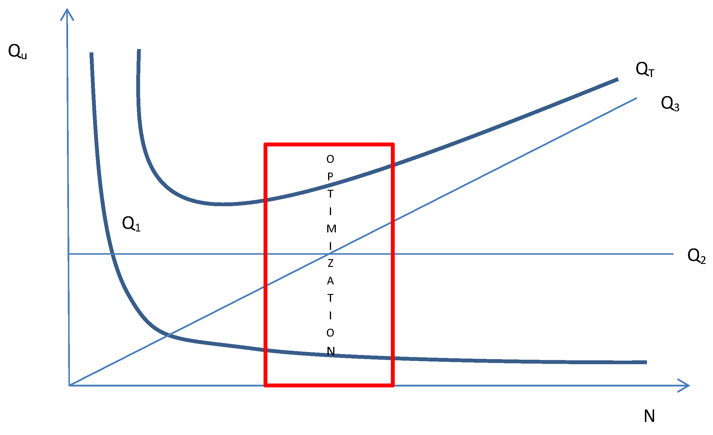
Comparing the three values to the number of produced pieces, it is possible to determine a hyperbole, a horizontal straight line, and a tilted line. Therefore, considering an economic set of production, the optimization is not in a narrow range. In this range, the curve is assimilable to a paraboloid, as shown in Figure 1.

After imposing a set of points that are approximately in the field of optimization of the set, it is possible to determine the real curve by assuming that the input data are far from it of a minimum constant value $6h$. In the diagram number of elements versus cost, we assume that there are four known points in the range of optimized production obtained experimentally, namely $\alpha$, $\beta$, $\gamma$, and $\delta$. We want to evaluate the value $6h$ of the approximation with the MaxInf principle. The inputs considered in this example are:

$$\left\{\begin{array}{c}\alpha (1650,133)\\ \beta \left(2250,131\right)\\ \gamma \left(2650,129\right)\\ \delta \left(3750,127\right)\end{array}\right.$$

(26)

where x is the number of mechanical elements and y is the unitary cost. Imposing that:

$$p\left(x\right)-y=\mp h$$

(27)

as a curve of constant error, or:

$$a{x}^2+bx+c\pm h=y$$

(28)

we have, alternatively:

$$\left\{\begin{array}{c}2722500a+1650b+c+h=133\hfill \\ 5062500a+2250b+c-h=131\hfill \\ 7022500a+2650b+c+h=129\hfill \\ 14062500a+3750b+c-h=127\hfill \end{array}\right.$$

(29)

and in matrix term:

$$\left[\begin{array}{cccc}2722500& 1650& 1& 1\\ 5062500& 2250& 1& -1\\ 7022500& 2650& 1& 1\\ 14062500& 3750& 1& -1\end{array}\right]\left[\begin{array}{c}a\\ b\\ c\\ h\end{array}\right]=\left[\begin{array}{c}133\\ 131\\ 129\\ 127\end{array}\right]$$

(30)

We obtain, as solution, the following parabolic curve:

$$p\left(x\right)=7.84314\times {10}^{-7}{x}^2-0.00737255x+143.324$$

(31)

where it is easy to verify that the value obtained with MaxInf principle is $h=-0.294118$. Thus, it is possible to calculate the curve of optimization that approximates with the max information. The goal of this example is, therefore, to achieve data on the cost-tolerance relationship. Comparative analysis with the mathematical model of Maxinf allowed us to control the cost existing for each set of the machining process.

7. Summary and Conclusions

In this paper, an approach to join together local design features using a mathematical model based on the MaxInf principle was proposed. In the data processing, the collection of particles, joined all together, constitutes a new cluster. By doing so, the three vectors of projections of $\overrightarrow{v_c}$ on coordinate planes was obtained in order to compute the vector of cluster $\overrightarrow{v_c}={\left[x_c,y_c,z_c\right]}^T$ using the MaxInf principle. The cloud of points can represent a sketch of industrial prototypes which can lead to an optimization of the design of new products. For instance, industrial prototypes having complex geometric shapes modeled using CAD systems allow for performing virtual simulations of rigid-flexible multibody systems using the multibody computational algorithms. Two simple examples are used for illustrating the method developed in the paper. In the first illustrative example, the MaxInf principle is applied to the extraction of the local features of a cluster of points. In the second demonstrative example, the Maxinf principle is employed to analyze costs related to the tolerances of mechanical components. The authors believe that the approach developed in the paper can be effectively used in the process of virtual prototyping and in the optimal design of mechanical systems.

References

- Shabana, A.A. Dynamics of Multibody Systems; Cambridge University Press: New York, NY, USA, 2013. [Google Scholar]
- Garcia De Jalon, J.G.; Bayo, E. Kinematic and Dynamic Simulation of Multibody Systems: The Real-Time Challenge; Springer: New York, NY, USA, 2012. [Google Scholar]
- Udwadia, F.E.; Kalaba, R.E. Analytical Dynamics: A New Approach; Cambridge University Press: New York, NY, USA, 2007. [Google Scholar]
- De Simone, M.C.; Rivera, Z.B.; Guida, D. Obstacle Avoidance System for Unmanned Ground Vehicles by Using Ultrasonic Sensors. Machines 2018, 6, 18. [Google Scholar] [CrossRef]
- Concilio, A.; De Simone, M.C.; Rivera, Z.B.; Guida, D. A new semi-active suspension system for racing vehicles. FME Trans. 2017, 45, 578–584. [Google Scholar] [CrossRef] [Green Version]
- Kulkarni, S.; Pappalardo, C.M.; Shabana, A.A. Pantograph/Catenary Contact Formulations. J. Vib. Acoust. 2017, 139, 011010. [Google Scholar] [CrossRef]
- Pappalardo, C.M.; Yu, Z.; Zhang, X.; Shabana, A.A. Rational ANCF Thin Plate Finite Element. J. Comput. Nonlinear Dyn. 2016, 11, 051009. [Google Scholar] [CrossRef]
- Pappalardo, C.M.; Patel, M.D.; Tinsley, B.; Shabana, A.A. Contact Force Control in Multibody Pantograph/Catenary Systems. Proc. Inst. Mech. Eng. Part K J. Multibody Dyn. 2016, 230, 307–328. [Google Scholar] [CrossRef]
- Guida, D.; Pappalardo, C.M. Forward and Inverse Dynamics of Nonholonomic Mechanical Systems. Meccanica 2014, 49, 1547–1559. [Google Scholar] [CrossRef]
- Pappalardo, C.M.; Wallin, M.; Shabana, A.A. A New ANCF/CRBF Fully Parametrized Plate Finite Element. J. Comput. Nonlinear Dyn. 2017, 12, 031008. [Google Scholar] [CrossRef]
- Ruggiero, A.; Affatato, S.; Merola, M.; De Simone, M.C. FEM Analysis of Metal on UHMWPE Total Hip Prosthesis During Normal Walking Cycle. In Proceedings of the AIMETA 2017—XXIII Conference of the Italian Association of Theoretical and Applied Mechanics, Salerno, Italy, 4–7 September 2017. [Google Scholar]
- De Simone, M.C.; Guida, D. On the Development of a Low Cost Device for Retrofitting Tracked Vehicles for Autonomous Navigation. In Proceedings of the AIMETA 2017—XXIII Conference of the Italian Association of Theoretical and Applied Mechanics, Salerno, Italy, 4–7 September 2017. [Google Scholar]
- Pappalardo, C.M.; Guida, D. On the Lagrange Multipliers of the Intrinsic Constraint Equations of Rigid Multibody Mechanical Systems. Arch. Appl. Mech. 2017, 88, 419–451. [Google Scholar] [CrossRef]
- Guida, D.; Nilvetti, F.; Pappalardo, C.M. Instability Induced by Dry Friction. Int. J. Mech. 2009, 3, 44–51. [Google Scholar]
- Pappalardo, C.M. A Natural Absolute Coordinate Formulation for the Kinematic and Dynamic Analysis of Rigid Multibody Systems. Nonlinear Dyn. 2015, 81, 1841–1869. [Google Scholar] [CrossRef]
- Guida, D.; Nilvetti, F.; Pappalardo, C.M. Dry Friction Influence on Cart Pendulum Dynamics. Int. J. Mech. 2009, 3, 31–38. [Google Scholar]
- Quatrano, A.; De Simone, M.C.; Rivera, Z.B.; Guida, D. Development and implementation of a control system for a retrofitted CNC machine by using Arduino. FME Trans. 2017, 45, 565–571. [Google Scholar] [CrossRef]
- Ruggiero, A.; De Simone, M.C.; Russo, D.; Guida, D. Sound Pressure Measurement of Orchestral Instruments in the Concert Hall of a Public School. Int. J. Circuits Syst. Signal Process. 2016, 10, 75–81. [Google Scholar]
- Pappalardo, C.M. Modelling Rigid Multibody Systems using Natural Absolute Coordinates. J. Mech. Eng. Ind. Des. 2014, 3, 24–38. [Google Scholar]
- Guida, D.; Nilvetti, F.; Pappalardo, C.M. Parameter Identification of a Two Degrees of Freedom Mechanical System. Int. J. Mech. 2009, 3, 23–30. [Google Scholar]
- Pappalardo, C.M.; Guida, D. Adjoint-based Optimization Procedure for Active Vibration Control of Nonlinear Mechanical Systems. J. Dyn. Syst. Meas. Control 2017, 139, 081010. [Google Scholar] [CrossRef]
- Guida, D.; Pappalardo, C.M. Sommerfeld and Mass Parameter Identification of Lubricated Journal Bearing. WSEAS Trans. Appl. Theor. Mech. 2009, 4, 205–214. [Google Scholar]
- Pappalardo, C.M.; Guida, D. Control of Nonlinear Vibrations using the Adjoint Method. Meccanica 2017, 52, 2503–2526. [Google Scholar] [CrossRef]
- De Simone, M.C.; Rivera, Z.B.; Guida, D. Finite Element Analysis on Squeal-Noise in Railway Applications. FME Trans. 2018, 46, 93–100. [Google Scholar]
- Pappalardo, C.M.; Wang, T.; Shabana, A.A. On the Formulation of the Planar ANCF Triangular Finite Elements. Nonlinear Dyn. 2017, 89, 1019–1045. [Google Scholar] [CrossRef]
- Guida, D.; Pappalardo, C.M. Control Design of an Active Suspension System for a Quarter-Car Model with Hysteresis. J. Vib. Eng. Technol. 2015, 3, 277–299. [Google Scholar]
- Pappalardo, C.M.; Wang, T.; Shabana, A.A. Development of ANCF Tetrahedral Finite Elements for the Nonlinear Dynamics of Flexible Structures. Nonlinear Dyn. 2017, 89, 2905–2932. [Google Scholar] [CrossRef]
- Guida, D.; Pappalardo, C.M. A New Control Algorithm for Active Suspension Systems Featuring Hysteresis. FME Trans. 2013, 41, 285–290. [Google Scholar]
- Pappalardo, C.M.; Guida, D. A Time-domain System Identification Numerical Procedure for obtaining Linear Dynamical Models of Multibody Mechanical Systems. Arch. Appl. Mech. 2018, 157, 232–235. [Google Scholar] [CrossRef]
- De Simone, M.C.; Guida, D. Modal Coupling in Presence of Dry Friction. Machines 2018, 6, 8. [Google Scholar] [CrossRef]
- Pappalardo, C.M.; Zhang, Z.; Shabana, A.A. Use of Independent Volume Parameters in the Development of New Large Displacement ANCF Triangular Plate/Shell Elements. Nonlinear Dyn. 2018, 91, 2171–2202. [Google Scholar] [CrossRef]
- Pappalardo, C.M.; Guida, D. On the Use of Two-dimensional Euler Parameters for the Dynamic Simulation of Planar Rigid Multibody Systems. Arch. Appl. Mech. 2017, 87, 1647–1665. [Google Scholar] [CrossRef]
- De Simone, M.C.; Guida, D. Identification and Control of a Unmanned Ground Vehicle by Using Arduino. UPB Sci. Bull. Ser. D 2018, 80, 141–154. [Google Scholar]
- Barbagallo, R.; Sequenzia, G.; Cammarata, A.; Oliveri, S.M.; Fatuzzo, G. Redesign and Multibody Simulation of a Motorcycle Rear Suspension with Eccentric Mechanism. Int. J. Interact. Des. Manuf. 2017, 12, 517–524. [Google Scholar] [CrossRef]
- Cammarata, A.; Sequenzia, G.; Oliveri, S.M.; Fatuzzo, G. Modified Chain Algorithm to Study Planar Compliant Mechanisms. Int. J. Interact. Des. Manuf. 2016, 10, 191–201. [Google Scholar] [CrossRef]
- Pappalardo, C.M.; Guida, D. System Identification and Experimental Modal Analysis of a Frame Structure. Eng. Lett. 2018, 26, 56–68. [Google Scholar]
- Pappalardo, C.M.; Guida, D. Dynamic Analysis of Planar Rigid Multibody Systems modelled using Natural Absolute Coordinates. Appl. Comput. Mech. 2018, 12. [Google Scholar] [CrossRef]
- Milosavljevic, B.; Pesic, R.; Dasic, P. Binary Logistic Regression Modeling of Idle CO Emissions in order to Estimate Predictors Influences in Old Vehicle Park. Math. Probl. Eng. 2015, 2015, 463158. [Google Scholar] [CrossRef]
- Dasic, P.; Dasic, J.; Crvenkovic, B. Service Models for Cloud Computing: Search as a Service (SaaS). Int. J. Eng. Tech. 2016, 8, 2366–2373. [Google Scholar] [CrossRef]
- Dasic, P.; Franek, F.; Assenova, E.; Radovanovic, M. International Standardization and Organizations in the Field of Tribology. Ind. Lubr. Tribol. 2003, 55, 287–291. [Google Scholar] [CrossRef]
- Dasic, P. Determination of Reliability of Ceramic Cutting Tools on the basis of Comparative Analysis of Different Functions Distribution. Int. J. Qual. Reliab. Manag. 2001, 18, 431–443. [Google Scholar]
- Serifi, V.; Dasic, P.; Jecmenica, R.; Labovic, D. Functional and Information Modeling of Production using IDEF Methods. Stroj. Vestnik/J. Mech. Eng. 2009, 55, 131–140. [Google Scholar]
- Dasic, P. Examples of Analysis of Different Functions of Cutting Tool Failure Distribution. Trib. Ind. 1999, 21, 59–67. [Google Scholar]
- Dasic, P.; Natsis, A.; Petropoulos, G. Models of Reliability for Cutting Tools: Examples in Manufacturing and Agricultural Engineering. Stroj. Vestnik/J. Mech. Eng. 2008, 54, 122–130. [Google Scholar]
- Zoller, C.; Dasic, P.; Dobra, R.; Pantovic, R.; Damnjanovic, Z. Sequential Algorithm and Fuzzy Logic to Optimum Control the Ore Gridding Aggregates. Tech. Technol. Educ. Manag. 2012, 7, 914–919. [Google Scholar]
- Lekic, M.; Cvejic, S.; Dasic, P. Iteration Method for Solving Differential Equations of Second Order Oscillations. Tech. Technol. Educ. Manag. 2012, 7, 1751–1759. [Google Scholar]
- Dasic, P.; Dasic, J.; Crvenkovic, B. Applications of Access Control as a Service for Software Security. Int. J. Ind. Eng. Manag. 2016, 7, 111–116. [Google Scholar]
- Pappalardo, M.; Villecco, F. Max-Ent in fast belief fusion. In Proceedings of the International Conference Differential Geometry, Dynamical Systems, Bucharest, Romania, 5–7 October 2007; Geometry Balkan Press: Bucharest, Romania, 2008; pp. 154–162. [Google Scholar]
- Villecco, F.; Pellegrino, A. Entropic Measure of Epistemic Uncertainties in Multibody System Models by Axiomatic Design. Entropy 2017, 19, 291. [Google Scholar] [CrossRef]
- Sena, P.; Attianese, P.; Pappalardo, M.; Villecco, F. FIDELITY: Fuzzy Inferential Diagnostic Engine for on-LIne supporT to phYsicians. In Proceedings of the 4th International Conference on the Development of Biomedical Engineering, Ho Chi Minh City, Vietnam, 8–10 January 2012; IFMBE Proceedings. Springer: Berlin, Germany, 2013; pp. 396–400. [Google Scholar]
- Sena, P.; Attianese, P.; Carbone, F.; Pellegrino, A.; Pinto, A.; Villecco, F. A Fuzzy Model to Interpret Data of Drive Performances from Patients with Sleep Deprivation. Comput. Math. Methods Med. 2012, 2012, 868410. [Google Scholar] [CrossRef] [PubMed]
- Ghomshei, M.; Villecco, F.; Porkhial, S.; Pappalardo, M. Complexity in Energy Policy: A Fuzzy Logic Methodology. In Proceedings of the 6th International Conference on Fuzzy Systems and Knowledge Discovery, Tianjin, China, 14–16 August 2009; IEEE: Los Alamitos, CA, USA, 2009; Volume 7, pp. 128–131. [Google Scholar]
- Villecco, F.; Pellegrino, A. Evaluation of Uncertainties in the Design Process of Complex Mechanical Systems. Entropy 2017, 19, 475. [Google Scholar] [CrossRef]
- Shabana, A.A. Computational Dynamics; John Wiley and Sons: West Sussex, UK, 2009. [Google Scholar]
- Piegl, L.; Tiller, W. The NURBS Book; Springer: Berlin, Germany, 2012. [Google Scholar]
- Pappalardo, M. Information in Metric Space. J. Mater. Proc. Technol. 2004, 157, 228–231. [Google Scholar] [CrossRef]
- Pappalardo, M.; Pellegrino, A. Application of Non-Probabilistic Information. J. Mater. Process. Technol. 2004, 157, 232–235. [Google Scholar] [CrossRef]
- Staiano, G.; Gloria, A.; Ausanio, G.; Lanzotti, A.; Pensa, C.; Martorelli, M. Experimental study on hydrodynamic performances of naval propellers to adopt new additive manufacturing processes. Int. J. Interact. Des. Manuf. 2018, 12, 1–14. [Google Scholar] [CrossRef]
Figure 1.
Cost diagram: unitary cost , number of elements N.
© 2018 by the author. Licensee MDPI, Basel, Switzerland. This article is an open access article distributed under the terms and conditions of the Creative Commons Attribution (CC BY) license (http://creativecommons.org/licenses/by/4.0/).
Share and Cite
MDPI and ACS Style
Villecco, F. On the Evaluation of Errors in the Virtual Design of Mechanical Systems. Machines 2018, 6, 36. https://doi.org/10.3390/machines6030036
AMA Style
Villecco F. On the Evaluation of Errors in the Virtual Design of Mechanical Systems. Machines. 2018; 6(3):36. https://doi.org/10.3390/machines6030036
Chicago/Turabian StyleVillecco, Francesco. 2018. "On the Evaluation of Errors in the Virtual Design of Mechanical Systems" Machines 6, no. 3: 36. https://doi.org/10.3390/machines6030036
Note that from the first issue of 2016, this journal uses article numbers instead of page numbers. See further details here.