Compton Composites Late in the Early Universe


1
Mayer Applied Research Inc., 1417 Dicken Drive, Ann Arbor, MI 48103, USA
2
Retired, 2260 Chaucer Court, Ann Arbor, MI 48103, USA
*
Author to whom correspondence should be addressed.
Galaxies 2014, 2(3), 382-409; https://doi.org/10.3390/galaxies2030382
Submission received: 17 April 2014
/
Revised: 25 June 2014
/
Accepted: 26 June 2014
/
Published: 15 July 2014
(This article belongs to the Special Issue Beyond Standard Gravity and Cosmology)
Abstract
:Beginning roughly two hundred years after the big-bang, a tresino phase transition generated Compton-scale composite particles and converted most of the ordinary plasma baryons into new forms of dark matter. Our model consists of ordinary electrons and protons that have been bound into mostly undetectable forms. This picture provides an explanation of the composition and history of ordinary to dark matter conversion starting with, and maintaining, a critical density Universe. The tresino phase transition started the conversion of ordinary matter plasma into tresino-proton pairs prior to the the recombination era. We derive the appropriate Saha–Boltzmann equilibrium to determine the plasma composition throughout the phase transition and later. The baryon population is shown to be quickly modified from ordinary matter plasma prior to the transition to a small amount of ordinary matter and a much larger amount of dark matter after the transition. We describe the tresino phase transition and the origin, quantity and evolution of the dark matter as it takes place from late in the early Universe until the present.
1. Introduction
There are a number of important and unanswered questions in this era of precision cosmology (see Schramm and Turner [1] and the texts of Kolb and Turner [2], Weinberg [3] and Rich [4]). Most mysterious is: what is dark energy? Somewhat less mysterious, but still requiring an answer is: what is dark matter? Another is: what accounts for the quantities of ordinary and dark matter? Finally: could some of these unanswered questions be related? In this paper, we propose an answer to the mysterious dark matter question from a new point of view, one very different from the now-standard Λ Cold Dark Matter (ΛCDM) cosmology (see [3] and [4], for example).
For some time, dark matter has been assumed to be one or another of a variety of non-baryonic relics left over from the very early Universe; it was considered to be a type of weakly interacting massive particle (WIMP). Therefore, there have been many investigations of various candidates, like neutrinos, axions, supersymmetric particles and others (see the discussions in Weinberg and Rich), but most have been found to be problematic when compared to cosmological and/or astrophysical observations. There have not been similar investigations late in the early Universe, because there was no identified low-energy process of change in later epochs. Furthermore, until now, efforts to detect some of these particles have not been successful.
In this paper, we introduce a new idea—that dark matter results, not from non-baryonic relics from the very early Universe, but from stable electromagnetic composite structures composed of a single proton and two electrons at the Compton-scale (a p-tresino) charge-balanced by a second proton—that is to say, two protons and two electrons, a type of WIMP. Other tresinos are introduced, as well. Our plan then is to describe how this composite system of paired-up and largely hidden baryons (for now, mostly protons) are generated and how the tresino phase transition proceeds in a late stage of the early Universe. We examine how the phase transition affects the composition of the evolving Universe and, also, how it is involved at much later stages in the Universe. We identify some astrophysical observations that are consistent with an origin in the phase transition. In particular, the tresino phase transition appears, even now, to be a powerful energy source, heating the solar corona to continue the conversion of ordinary into dark matter.
For completeness, in Section 2, we briefly describe the bound-state tresinos () and introduce the second important Compton-scale tresino, a proton-tresino () that, unlike its bound-state cousin, is a short-lived resonant scattering state; we show how the proton-tresino (hereafter referred to as a ptre ) is the precursor of the bound-state tresino. Both tresinos are necessary to generate dark matter late in the early Universe and later in astrophysics. In Section 3, we examine the ptre population with an unphysical, but useful, preliminary calculation. In Section 4, we describe the completion of the phase transition, for a realistic physical picture. We describe the formation and importance of rotors and their evolution in Section 5. The phase transition and nucleosynthesis is discussed in Section 6 and its effect at the Cosmic Microwave Background (CMB) in Section 7. The transition’s connection to the solar corona is described in Section 8, and some final discussion on the implications of the transition on this cosmological picture are presented in Section 9.
Appendix A presents a heuristic model for the ptre. The Saha–Boltzmann equilibrium derivation for the baryon composition is presented in Appendix B. A few characteristics of proton-tresino molecules (PTMs) and rotors as dark matter are presented in Appendix C, and a connection between the PTMs and some astrophysical observations in the infrared are presented in Appendix D.
In this paper, we consider a critical density, flat, Universe. The tresino phase transition begins from the matter density and converts most of the matter into proton-tresino pairs and a small amount of ordinary matter. Collisions between proton and tresino populations then evolve into rotating pairs (rotors). Some of the rotors “spin-down” to form proton-tresino molecules (PTMs). Therefore, throughout the transition, , with representing the ordinary matter fraction and the dark matter fraction, both relative to critical density. Thus, flatness is maintained throughout with no dark energy required.
Readers will note that the tresino phase transition represents a modification of the usual adiabatic big-bang scaling, i.e., and , subscripted parameters referring to the present values of baryon density and temperature and have been taken to be input quantities, rather than being determined from the cosmological model. In our big-bang picture, the influence of the tresino phase transitions are taken into account, making it a non-adiabatic model. Therefore, and are treated not as inputs, but, rather, determined from the model, and of course, they must agree with observations at . Specifically, we show that the baryon density, , is substantially smaller than it was in earlier eras, yet agrees with cosmological observations, including the production of dark matter and nucleosynthesis.
2. Tresinos: Bound and Resonance Types
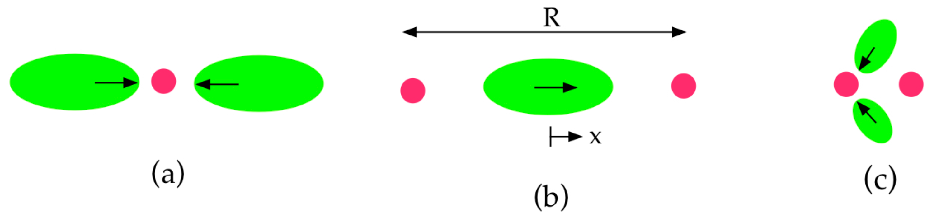
We begin by briefly describing the physics behind the the three-particle composites that we call tresinos—the bound-state tresino () is detailed in our recent paper (Mayer and Reitz (M&Ra)) [5] , shown schematically in Figure 1a. However, in addition to the bound-state tresino, there is a scattering-resonance tresino with transposed particles, a proton-tresino () or ptre, for short, composed of two protons and an electron, shown schematically in Figure 1b. The latter composite is a three-body quantum system that is too complex to admit a straightforward quantum mechanical solution. In this paper, we present heuristic models for both tresinos, assuming that they are physically, but not quantum mechanically, precise.
Figure 1.
Classical depictions of the electromagnetic configurations for (a) the tresino, (b) the ptre and (c) the proton-tresino molecule (PTM) with individual components, protons in red and electrons in green.
Figure 1.
Classical depictions of the electromagnetic configurations for (a) the tresino, (b) the ptre and (c) the proton-tresino molecule (PTM) with individual components, protons in red and electrons in green.

The scattering resonance ptre is considered to be an “Efimov state” [6] at the Compton scale. An Efimov state can be described as a resonant scattering of three particles, none of whose two-particle sub-groups have to be stable. Note that such a state at the atomic scale has apparently been recently observed experimentally (see Kraemer, et al. [7]) and, as expected, at rather low particle densities. It is believed that Efimov states can take on a number of different shapes, including linear (see Appendix A). Needless to say, three-body composites in either bound states or scattering states, are very difficult quantum mechanical calculations (for example, see Nishida, et al.[8]), so in both systems, we resort to heuristic models in order to provide guidance for later efforts.
Below, we describe how the ptre is the precursor of the bound-state tresino. Both tresinos are Compton-scale composites; the tresino being composed of two electrons and a proton bound together by electromagnetic forces, whereas the ptre is composed of two protons and an electron in a resonant scattering (Efimov state). Figure 1a is a classical depiction of the tresino configuration; a quantum mechanical model has been presented and discussed in our recent paper (M&Ra). It is important to note that the tresino is a bound state with a net negative charge and is quite small (Compton scale); it has a binding energy of one Compton energy unit, keV. Being a three-body electromagnetic entity assembled from a proton and two electrons, tresinos are not easily, or usually, formed. However, the tresino formation energy may be the dominant energy source of thermal heating in the Earth (Mayer and Reitz (M&Rb) [9]). The formation and the release of the tresino binding energy, in the Earth, is made possible by the high concentration of protons and free electron pairs, both as components of specific ions. On the other hand, the plasma of the early Universe is a quite different place with a unique environment for the formation of tresinos and later for charge-neutral proton-tresino molecules (PTMs) (Figure 1c). This latter combination obtains because negatively-charged tresinos and positively-charged protons are, of course, attracted to each other; see Appendix C.
In M&Ra, we also described the He-tresino composed of two electrons and a nucleus (α particle). The α-tresinos are charge-neutral and more strongly bound ( keV) than are the more numerous p-tresinos; they also play a role in tresino nucleosynthesis (see Section 4.1 and Appendix B).
As we now focus on the more abundant p-tresinos, there are a number of characteristics of this bound-state tresino to keep in mind. First, it is held together by a balance of electrostatic and magnetic forces. Second, at formation, it releases the binding energy and must gain it back to be disassembled. It is negatively-charged, has a mass about equal to that of the proton and has no excited states. Therefore, each p-tresino formed releases 3.7 keV as recoil kinetic energy. Finally, the p-tresino radius is several Comptons; the natural scale of these electromagnetic composites is the electron Compton wavelength, cm. Hence, it is small on the scale of atoms, large on the scale of nuclei and appears to have no excited states. This last characteristic was the reason for considering tresinos as participants in the generation of dark matter.
Appendix A details a heuristic model of the ptre as an Efimov scattering resonance; it is useful for envisioning the later conversion to a p-tresino. As a resonant scattering or metastable system, the ptre has a natural lifetime; it persists for this period, so long as it does not experience a collision. Two types of collisions are possible: the first, and most common, is one that destroys the ptre, thereby returning it to its original components. The second, and least common, type of collision occurs when the incident particle is a second electron impacting either ptre proton at a time when the metastable trapped-electron is sufficiently close to this proton. If the spins are correctly aligned, then this electron plus the electron already resident in the ptre may collapse to form a tresino. This collision then releases the tresino binding energy to the newly-created tresino and its nearby proton. The binding energy is carried away as the recoil kinetic energy of the newly formed tresino and the nearby proton. The ptre to tresino transition can be relatively frequent if the electron density is high, or it can be infrequent when it is low; but, with sufficient time during the plasma expansion, this transition eventually occurs and releases its binding energy; or if an electron or another particle destroys the ptre, another may form again later to take its place. As we find below, the time available to complete the phase transition is sufficient in this era. The collision modifications are presented below after we have described the first stage of the transition dynamics.
3. The First Stage: The ptre Population
Consider the sequence of events leading up to the ptre to tresino transition. First, the resonant scattering collisions combine electrons and protons into ptres. If this process were to continue indefinitely or if the ptre had an infinite natural lifetime, the evolving plasma would eventually be composed of only ptres and an equal number of electrons. In order to make clear how the transition proceeds, we begin by presenting this initial phase of the transition as if there were no electron collisions converting ptres into tresinos; then, we modify it to complete the transition. Therefore, Section 3 is not physically correct, but we present it to make the transition process, which proceeds in two steps, somewhat more transparent; we correct this in Section 4.
Using the Saha–Boltzmann equilibrium (see Equation (B7)), we evaluate this first “unphysical” situation for the populations of ptres, protons and electrons, starting from a time much later than the era of primordial nucleosynthesis. The equilibrium combination equation is:
where is the ratio of electrons to baryons, is the ratio of protons to baryons and is the ratio of ptres to baryons, and these populations are z-dependent through a modified big-bang scaling,
We have introduced the critical baryon number density , consistent with , rather than the usual (adiabatic) , the baryon number density at . As we show, the phase transition converts almost all of the baryons prior to the transition into dark matter with only a small amount of ordinary matter, , making it through the transition.
Notice, in Equation (1), that the transition takes place as x ranges over . With , keV and K, we find that the ptre transition begins close to , corresponding to roughly two hundred years after the big-bang. At this time, the plasma density and temperature have fallen to a few times and 25 eV, respectively. As noted, the tresino phase transition begins from the matter density and converts most of the matter into proton-tresino pairs with some smaller amount of ordinary matter. Recalling again that throughout the transition , with the ordinary matter fraction and the the dark matter fraction.
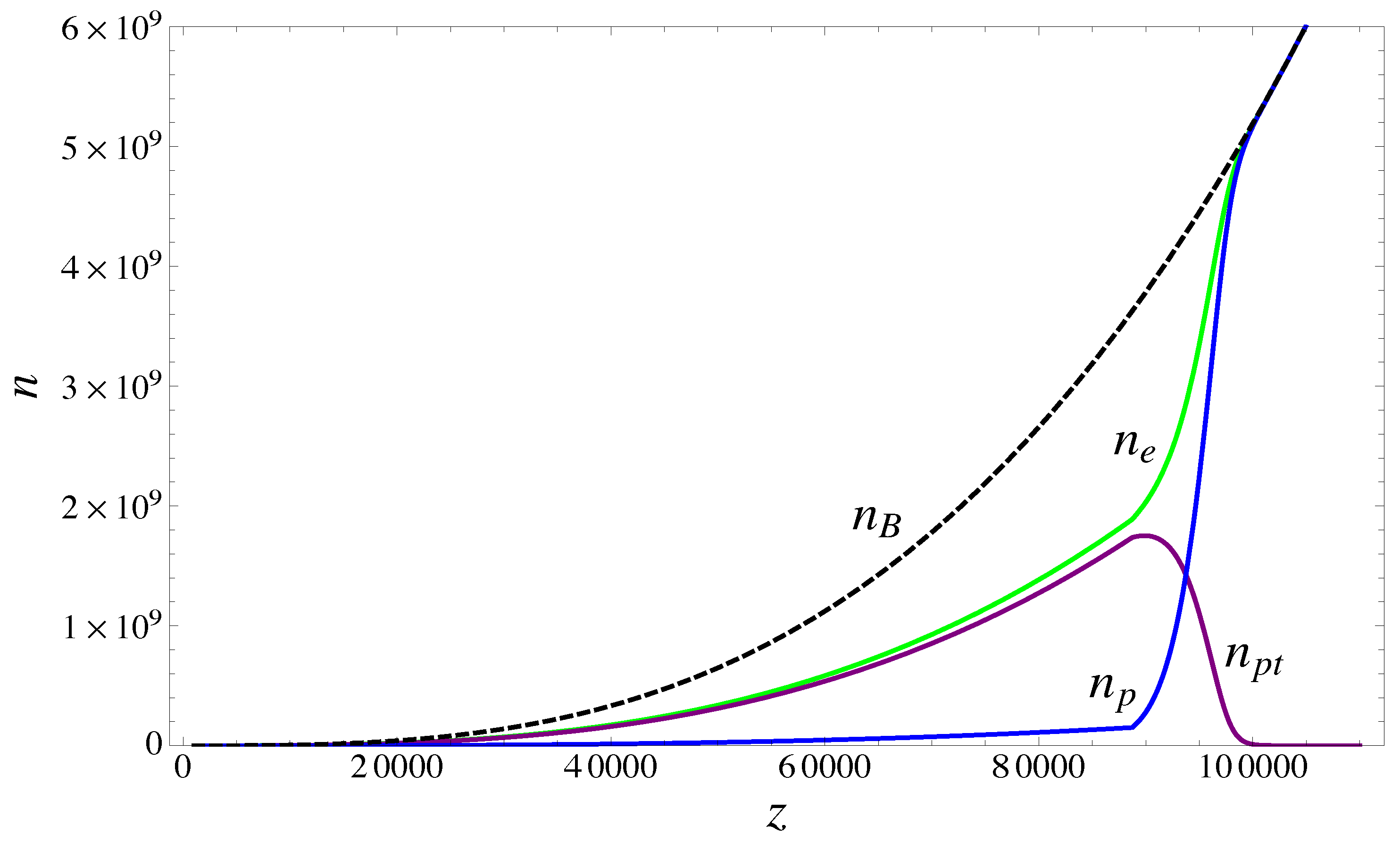
The evaluation of the equilibrium ptre combination of Equation (1) is shown in Figure 2. The ptre combination is seen to be mostly completed over the period , or about a 200 year period. As expected, the composition of the evolving plasma has changed; the baryons are conserved, though the proton density has been depleted, and only ptres and electrons remain. However, these populations are “unphysical”; they represent the first step of the ptre to tresino transition within the equilibrium assumption. We present the second step modification to the phase transition in the next section; it provides a physically acceptable evaluation.
In the following figures, the dashed-black curves denoted represent the baryon density as if no tresino transition took place; so, they agree with the usual baryon scaling for , but are considerably different at smaller z.
Figure 2.
Evaluation of the equilibrium Saha–Boltzmann ptre combination displaying the proton density in blue, the electron density in green, the ptre density in purple and in dashed-black, with , , K.
Figure 2.
Evaluation of the equilibrium Saha–Boltzmann ptre combination displaying the proton density in blue, the electron density in green, the ptre density in purple and in dashed-black, with , , K.

4. Completing the ptre to Tresino Transition
Note that the electron-ptre collision rate is very fast on the time-scale of the expansion of the Universe. Practically then, as soon as a ptre is formed, it will be converted to a tresino. In short, tresinos quickly replace ptres as the transition proceeds. Each ptre to tresino conversion releases 3.7 keV of recoil kinetic energy to the tresino-proton pair. Therefore, the transition then evolves a new energetic population of tresinos and protons along with the surviving ordinary matter. The plasma composition and energetics are therefore changed and have to be accounted for in the co-moving frame.
First, we modify the various components to account for the electron collisions that convert ptres to tresinos. This particle accounting is accomplished by: (1) subtracting one electron from the population for each tresino created; (2) adding one proton for each tresino created; and (3) converting one ptre for each tresino created. These transformations, in the notation defined below Equation (1), read as follows:
Note that in this now-transposed system, the plasma evolves such that, if continued indefinitely, it would be comprised of only tresinos and protons. In fact, this situation almost obtains. However, when the electron density falls to a low value as they are used-up in the transition, a point is reached where newly formed ptres are not converted to tresinos, because of the now too-infrequent electron collisions. Exactly where this occurs is difficult to determine in our equilibrium model, so we introduce a cut-off parameter, β, such that no further transitions take place after the electron density has fallen below a fraction β of the proton density; a useful approximation for further numerical evaluations.
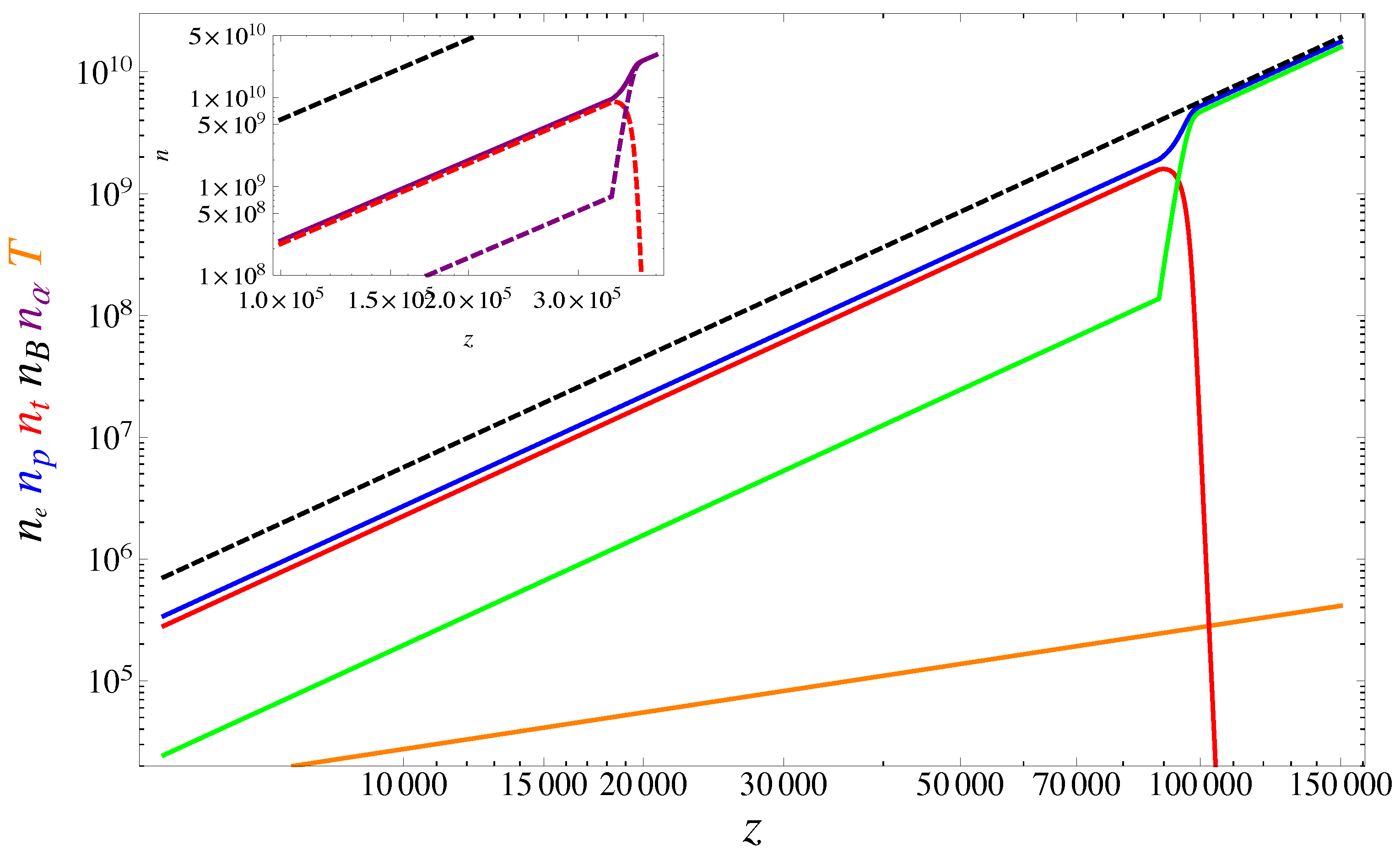
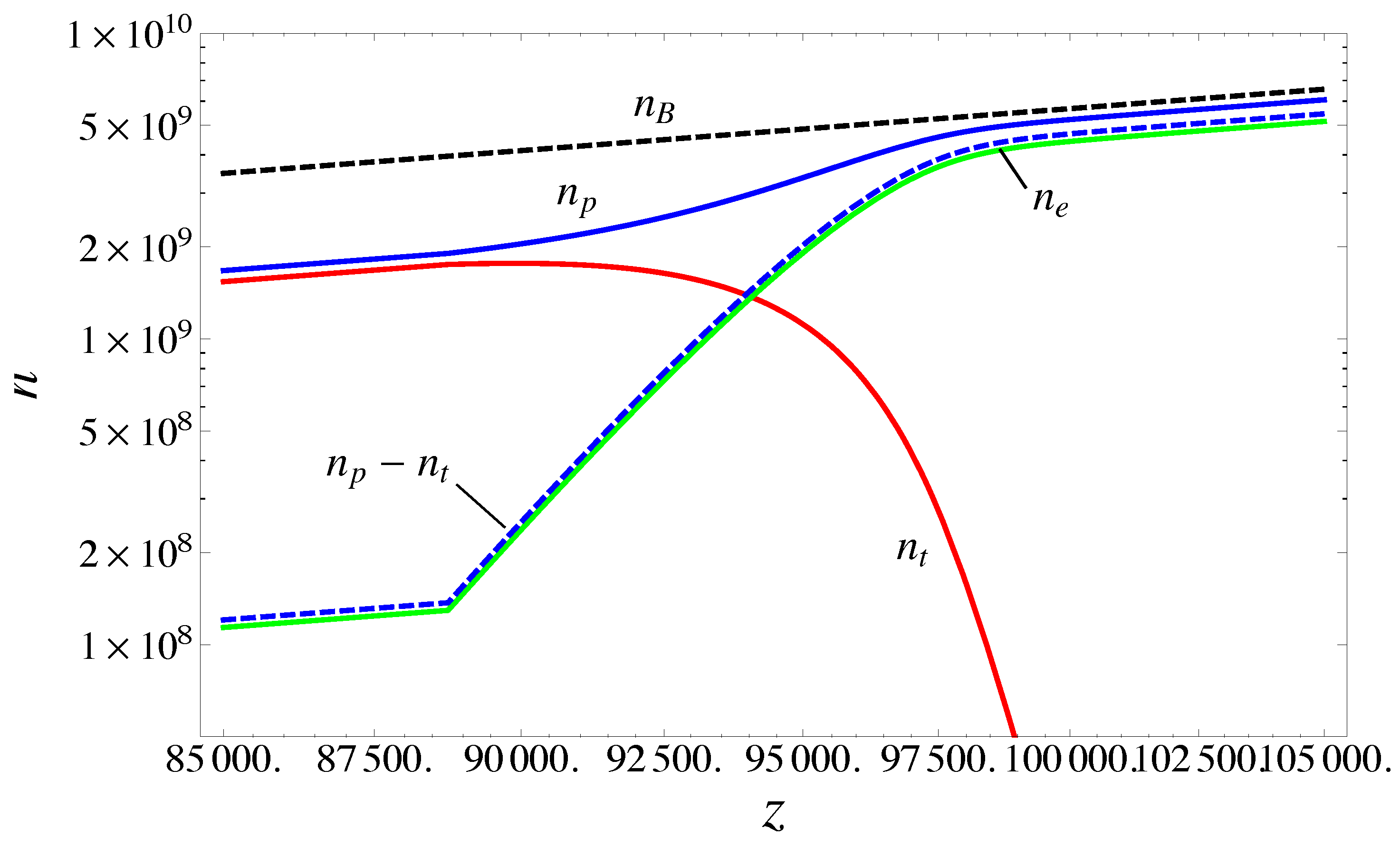
Figure 3 and Figure 4 present the evaluation of the Saha–Boltzmann equilibrium combination with and . The usual adiabatic scaling of density is shown in dashed-black. Notice that the ptre to tresino transition now takes place in the relatively short period when the plasma temperature (shown in orange) has fallen to about 25 eV and the density to about /cm. Further, notice that after the transition is complete, the plasma consists of three constituents, protons, tresinos and some smaller numbers of electrons (smaller by the same amount, as the proton numbers are greater than the tresino numbers). By charge neutrality, there are two groups of protons, those balanced by tresinos and those balanced by electrons. The latter group is shown in Figure 4 as the curve and represents the ordinary matter in this picture. The important point is that most of the baryons before the transition have now been transformed into proton and tresino pairs with only a small fraction (about 4%) continuing on as the ordinary matter fraction to the present. This new composition then continues on to lower z, where, eventually, recombination of the surviving electrons and protons takes place, in the usual way, and CMB photons are released. However, notice that at recombination (), the CMB has a baryon density considerably smaller than it had prior to the transition. Therefore, before the transition and after the transition.
Figure 3.
Numerical evaluation of the equilibrium Saha–Boltzmann tresino combination displaying the proton density in blue, the tresino density in red, the electron density in green, the temperature K in orange, and in dashed-black, with , and (see text). Note: the tresino and electron densities have been reduced by 10% for graphical clarity. The inset displays the (earlier) α-tresino generation in dashed red from He in purple (see Section 4.1 and Appendix B).

Data reduction from the Wilkinson Microwave Anisotropy Probe (WMAT) measurements [10], using the standard model, found the ordinary matter fraction to be about four percent, so we have chosen in the above and subsequent evaluations. Had we chosen another value of β, a different ordinary matter fraction at would have resulted.
Figure 4.
The same as Figure 3, but on a finer scale through the transition with the electron density in dotted green and the ordinary matter part of the proton density in dashed blue (see text). Note: the latter density has been reduced by 10% and the electron density by 15% for graphical clarity.
Figure 4.
The same as Figure 3, but on a finer scale through the transition with the electron density in dotted green and the ordinary matter part of the proton density in dashed blue (see text). Note: the latter density has been reduced by 10% and the electron density by 15% for graphical clarity.

4.1. Helium Tresinos
As in standard big-bang nucleosynthesis (SBBN), baryogenesis (with ) initially creates protons and neutrons that, at this high-density, form mostly He nuclei, but few other low-mass nuclides (see, for example, Rich’s [4] Figure 6.7, page 222). Then, roughly 40 years after the big-bang, the density fell to the point where most of the available He nuclei are transformed into He-tresinos (or α-tresinos). Note that we had first described the He-tresinos in M&Ra. Now, using the equilibrium derivation (see Appendix B), in the same manner as presented for the proton-tresinos above, it is straightforward to evaluate the He-tresino modification to the evolving plasma. The result of this early He-tresino modification is shown in the insert in Figure 3. As with the later arriving p-tresino transition, the He-tresino transition adds substantial recoil kinetic energy to the evolving plasma. On the other hand, the He-tresinos are neutral; hence, they do not orbit with a partner as do the p-tresinos.
The protons, He-tresinos and a now smaller number of He then continue on. The ratio of He-tresinos to He nuclei depends upon a cut-off parameter similar to the β chosen above. Without such a cut-off, there would be no He in our Universe, just as in the case of the p-tresino transition. Therefore, we again choose for the He-tresino transition; this results in a proton density about three times that of He, close to the presently observed ratio. Then, a few hundred years after the He-tresino transition, the p-tresino transition appears (see Figure 3).
5. Post-Transition Plasma and Dark Matter History
The equilibrium model presented in Section 4 has substantially modified the composition of the evolving plasma. After the p-tresino transition ends, the plasma is composed of tresinos, protons, photons and a small amount of ordinary matter. If there were no further interactions, the plasma beyond the transition would appear very much like that of Figure 3. However, there are still collisions between these populations as the plasma continues to expand. Especially important are the collisions between tresinos and protons, since they are roughly equal in numbers and are attracted to each other. The tresinos and protons eventually pair-up to form rotating pairs (rotors) and later into PTMs. We characterize the dominant post-transition plasma modification in the following subsections. A smaller, but important, tresino transition modification, namely nucleosynthesis, is discussed in Section 6.
5.1. Rotor Lifetimes
Throughout the tresino transition, and beyond, there are collisions between tresinos and protons. These two particles will orbit each other as rotors and spin-down releasing photons as they do so. We quantify the dynamics of this process in Section 5.2, but first, we outline a simplified picture of this radiative energy loss as a cyclotron radiation process. We note that during spin-down, the system is actually increasing its orbital kinetic energy in the potential well, as the energy is radiated away.
The slow energy loss of a proton in a constant magnetic field () is straightforward, starting from the cyclotron power loss (see, for example, Marion and Heald [11]) of a particle in a circular orbit. The calculation results in an exponential energy loss,
where τ is the characteristic energy loss time scale and is the proton’s initial energy. However, for a proton orbiting in the tresino electron’s magnetic dipole field, as the proton spins down, the magnetic field strength increases as the two particles come closer together. We make a simple, but crude, modification to the calculation just described, by allowing the magnetic field to scale as,
This calculation results in a linear energy loss going as , but where τ is the same as that of the constant magnetic field example given above. The point is that the energy-loss time scaling with the magnetic field continues as,
but now, the rotational energy is fully exhausted in one τ unit. Other inverse power law magnetic fields vs. energy loss behave in a similar manner.
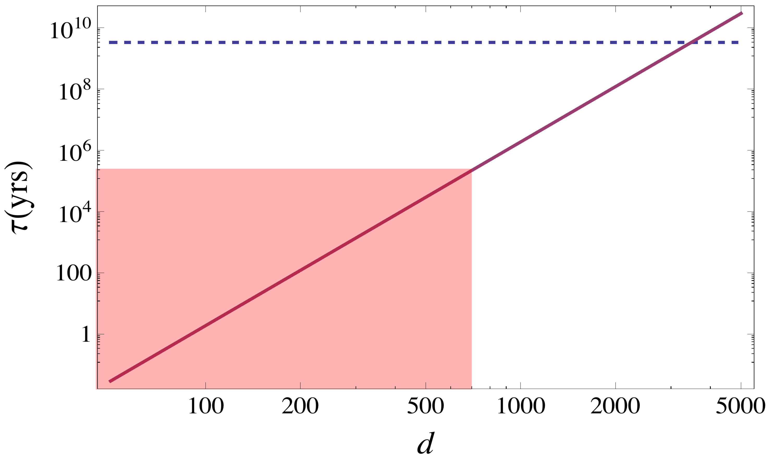
With this approximate scaling, we substitute the magnetic dipole field of the tresino’s electrons to estimate the energy-loss time in the spin-down of the rotors until they finally become PTMs. The electron’s dipole magnetic field goes as , so introducing this into τ and measuring the distance d (in Comptons) between the rotor’s proton and tresino, we find a crude estimate for the energy-loss times for rotors plotted in Figure 5, starting from various initial distances (impact parameters) d apart. Note the extremely long spin-down times for those rotors having impact parameters ; some rotor spin-downs persisting even until , as indicated by the dashed line in Figure 5. Some rotors may not have completely spun-down even now. Further, notice that a sufficiently large impact parameter implies no rotor formation, hence no spin-down to PTMs. This situation is the same as having a fraction of the protons and tresinos remaining too far apart and, therefore, not charge-neutralized for a very long time. Those rotors starting with sufficiently large ds will later be indistinguishable from a free tresino-proton plasma.
Figure 5.
The energy-loss lifetimes for proton-tresino rotors having initial impact parameters a distance d (in Comptons) apart. The shaded region indicates those rotors with sufficient time to spin-down prior to the recombination era. For reference, the dashed line locates .
Figure 5.
The energy-loss lifetimes for proton-tresino rotors having initial impact parameters a distance d (in Comptons) apart. The shaded region indicates those rotors with sufficient time to spin-down prior to the recombination era. For reference, the dashed line locates .

5.2. Rotor Spin-Down Dynamics
Here, we present a schematic, semi-classical, rotor spin-down model; it assumes a simple rotational balance between electrostatic attraction and the centrifugal force. Consider that a proton and tresino collide with an impact parameter initially a distance d apart. The force balance equation and angular momentum are:
where μ and r are the reduced mass and the center of mass distance, respectively. It is easy to show that the angular momentum can be rewritten and substituting the numerical values , where we have introduced the normalized radius with the Compton wavelength. It is useful to associate L with Planck’s constant by taking , so that, then, . The latter is a natural assignment, because, as the rotor spins-down, it must release a unit of angular momentum for each photon released. With this identification, it is easy to show that the and the rotational energy levels can be written as, , where , i.e., the Compton energy unit.
We can now write the energy level change per photon release as:
The spin-down of a rotor therefore goes through a sequence of levels starting from a largest radius (half of the impact parameter), say , and ending at a smallest radius, say , as the radius contracts by with each photon release. If there were no further interactions from the rotor spin-down starting at until now, the redshifted radiation frequency spectrum is well fitted by a spectral index form, , with GHz and GHz. This spectrum was determined as the spin-down of a rotor, whose starting radius was and whose ending radius is at . We note that this spectrum and spectral index are similar to some astrophysical observations at wavelengths far below the CMB radiation; the observed spectra are commonly considered to have resulted from synchrotron radiation from relativistic electrons in interstellar magnetic fields (for example, see Kogut [12] and Strong, et al. [13]). However, some part of the observed long-wavelength radiation spectra might be attributable to relic rotor spin-down photons.
5.3. Rotor Photons at Recombination
Now, we estimate the numbers of the spin-down photons at the recombination era, at the formation of the CMB. Again, recall that ours is an equilibrium model. It gives the tresino and proton densities, but does not specifically account for their assembly into rotors, a process that removes both tresinos and protons as expansion proceeds. Hence, we can only estimate the radiation numbers according to some averages over the expected populations near their peaks.
First, note that the spin-down radiation has traveled along with the remaining ordinary matter, since the transition started. However, the ordinary matter is now only a small fraction of its amount prior to the transition; that is, the transition has transformed most of the matter into the tresino and proton pairs. Although there will undoubtedly be some interaction with the ordinary matter during the expansion down to the recombination era, these interactions are outside the scope of this paper, and so, we neglect them in the following discussion.
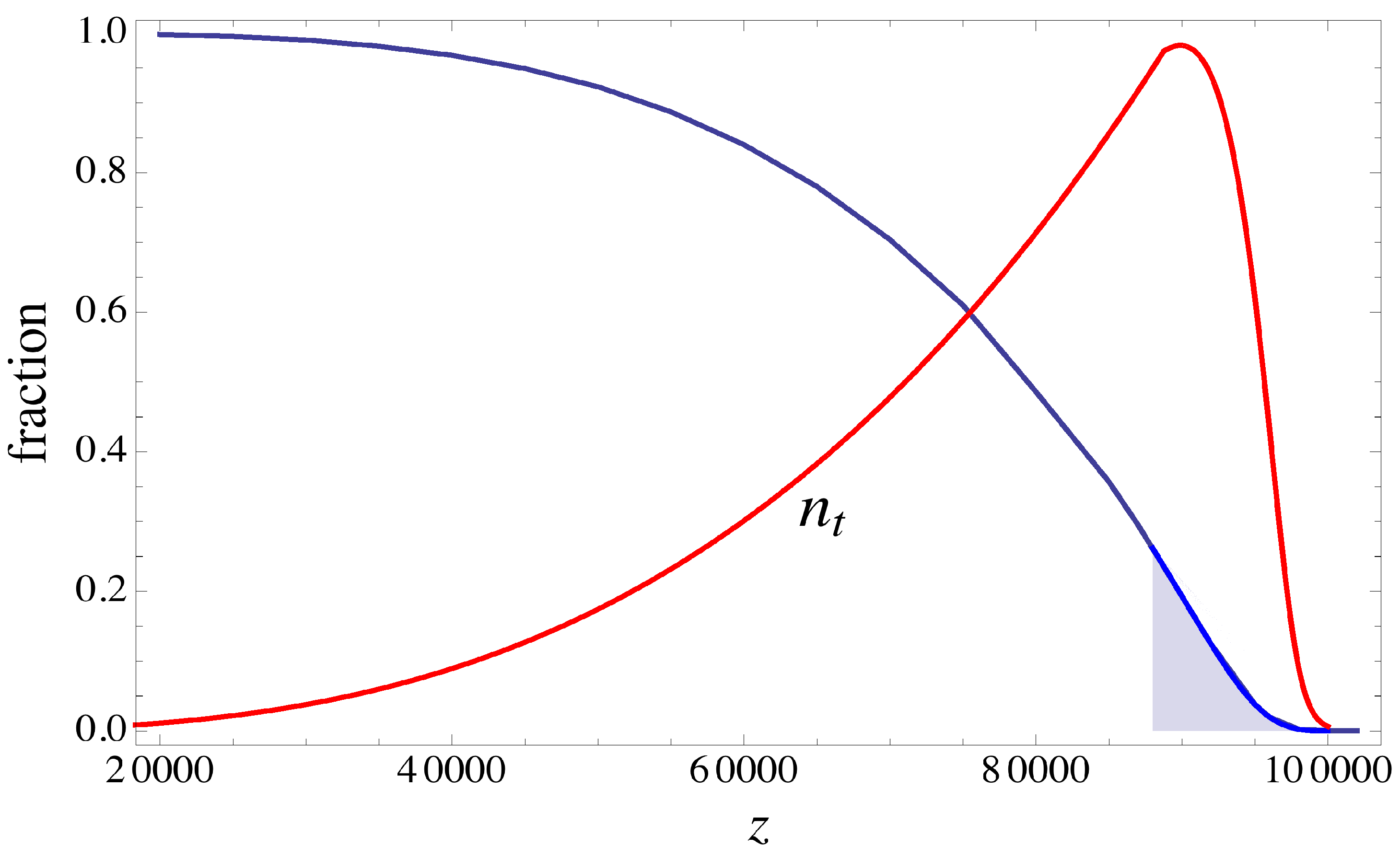
In Figure 6, the red curve shows the tresino density (about equal to the proton density) normalized to the peak () of the transition zone at . However, tresino-proton pairs are generated both earlier and later than at the peak, so we integrate across the peak to estimate the total numbers generated near the peak. This is the point at which the two species are most closely intermixed (the inter-particle spacing for both, at the peak, is roughly 7 μm). The blue curve shows the integrated numbers of tresinos through the transition. We assume that the number densities of the rotors are proportional to the integrated tresino densities across the peak (the shaded zone in Figure 6). The tresino numbers, integrated across a band around the peak is:
Note also that the rotors formed in this peak zone amount to about 26% of the total produced throughout the transition.
Now, assuming that each of these tresinos forms a rotor in a proton collision at different diameters, the rotor spin-down photon numbers will be:
where, as in the example of Section 5.2, is the smallest and is the largest rotor diameter. For a particular example, take and ; then, the total number density of spin-down photons is about .
Figure 6.
A plot of the fraction of integrated tresino number density (blue curve) and the tresino density (red curve) through the transition. The shaded zone is the region of the rotor production averaging (see the text).
Figure 6.
A plot of the fraction of integrated tresino number density (blue curve) and the tresino density (red curve) through the transition. The shaded zone is the region of the rotor production averaging (see the text).

Next, let us consider the spin-down photon density at the time of recombination and compare it to the CMB photon density. The spin-down photon density at recombination will be down by a factor of , giving it a density of . The CMB photon density, on the other hand, is about , so the ratio of spin-down photons to CMB photons is about a factor of 10. Noting again that the spin-down photon spectra lies below the reddest end of CMB spectrum. Spin-down photons from the tresino transition are not accounted for in the standard model at the release of the CMB photons.
The tresino-proton rotor calculation above is illustrative, but is inaccurate for a number of reasons. First, the rotors at different z’s, even around the peak, will be redshifted by different amounts. Second, there would have to be a better averaging of the various spin-down summations, whereas we have treated them all equally. Finally, we have not accounted for the influence of the spin-down photon scattering on the remaining ordinary electron population or other interactions along the way from the transition to recombination. An important issue (noted by a reviewer) is the possibility of rotors being spun-up some time during or after the transition. At present, we do not know of a the cross-section model for this interaction. Another issue is the equilibration and energy redistribution of spin-down photons; a difficult problem that will require further work. The low-electron densities after the transition could be less-effective than might be expected, but some energy gain and thermalization of spin-down photons (Comptonization) might be provided by photon scattering on the bound electrons of the tresino, because of their much larger numbers compared to electrons. Much more work is required to resolve the late-time effects of the tresino transition.
Finally, we note again that all of the radiation from rotor spin-down has originated from the release of the binding energy in the tresino formation. Since all of the spin-down radiation has originated from this release, the sub-CMB long-wavelength radiation amounts to roughly a few keV from each tresino-proton pair that was created.
5.4. Plasma Beyond Recombination
The time between the tresino phase transition and recombination era is about years. Note from Figure 5 (Section 5.1) that this time corresponds to a maximum rotor diameter of . For rotors with larger ds, the spin-down will not have had time to be completed. Therefore, these rotors may not be observed in CMB observations, like WMAP. The fraction considered to be dark matter in WMAP data is estimated at about 26% of the critical density. This fraction could have been all of those rotors having . The remaining 70% might have been those rotors with (Figure 5). This group might have gone unobserved in the CMB data and gone on to populate the later Universe. Note that rotors with sufficiently large ds would be indistinguishable from a plasma composed of tresinos and protons, except perhaps for some currents, hence magnetic fields (see Section 8). The important issue of transition nucleosynthesis is addressed in Section 6.
In summary, beyond the recombination era, late in the early Universe, the plasma composition includes a small amount of ordinary matter (some as low-mass nuclides from the transition nucleosynthesis of Section 6), CMB radiation, the PTMs and its radiation, incompletely spun-down rotors and a residual low-density plasma of tresinos and protons. Determining the quantities of each of the hidden or dark matter species will require a more complete, non-equilibrium calculation of the post-transition plasma composition than we have presented here.
As mentioned, we do not invoke dark energy in this model; we are quite aware that this is not consistent with an accelerating Universe. In particular, it is not consistent with the Supernovae (SN Ia) data indicating acceleration (see Riess, et al. [14] and Perlmutter, et al. [15]). On the other hand, our picture does agree with a number of other observations both cosmological and astrophysical and is less mysterious than dark energy. It is also possible that there is still residual extinction by some rotors still spinning-down closer to our present era.
5.5. Detecting the Post-Transition Dark Matter Particles
With the composition of the post-recombination plasma just presented, we make a few comments on the detection of the various components of our dark matter species, noting that we expect this to be a difficult task. First, consider the PTMs that arrive in our local neighborhood. They are quite small, have the mass of hydrogen molecules, are quickly thermalized and, like hydrogen, will escape the atmosphere. In a similar fashion, incompletely spun-down rotors will also escape the atmosphere. Next, consider the tresino-proton plasma. The protons and tresinos will have cooled, by expansion, to low energies. Protons and tresinos entering our local neighborhood will be neutralized in our high-density atmosphere; a proton by grabbing an ambient electron to become neutral hydrogen and the tresino by grabbing an ambient proton to become a rotor. We expect both species will remain hidden, except perhaps in deep-space experiments. These characteristics of our dark matter species could make it difficult to field direct detection experiments.
6. Nucleosynthesis in Tresino-Transition Cosmology
There are three nucleosynthesis eras in our cosmological model. The first is the primordial baryon and lepton synthesis that proceeds very early, just as in the standard model [3]. Then, much later, after the density and temperature have fallen substantially, the He-tresino transition arrives. Finally, later still, the much larger p-tresino transition arrives. This last era generates the low-mass nuclides, as we show below. To simplify notation, from here on, we will refer to hydrogen-tresinos () and the helium-tresinos () with asterisks.
In an earlier version of this paper, a reviewer pointed out that there could be a conflict between the tresino phase transition and the much earlier standard big-bang nucleosynthesis (SBBN) era. The low-mass nuclide abundances have been calculated from well-characterized fusion reaction physics (see Section 6.5 of Rich [4] and Section 3.2 of Weinberg [3]) and the SBBN calculations compare well with observations (considered a major success of big-bang theory). This criticism would, of course, be fatal to our high-density cosmology if nucleosynthesis could only have occurred in the very early universe. However, in this Section, we show that the unique characteristics of tresinos provide an alternative to standard big-bang nucleosynthesis. Specifically, nucleosynthesis that generates the relatively small numbers of low-mass nuclides during the peak of the tresino phase transition as baryon conversion to dark matter takes place. We emphasize again that considering η, the baryon to photon ratio, to be conserved throughout the expansion (as done in SBBN), presumes the usual adiabatic BB picture. On the other hand, our model conserves total baryons, but most are converted to dark matter during the and tresino transitions.
As noted in M&Ra, when tresinos are generated, nuclear reactions that were strongly inhibited by the Coulomb barrier may be instead promoted due to the ability of the tresino’s bound electrons, through polarization, to escort tresinos into nuclear collisions. Furthermore, we showed that the two bound electrons quite frequently reside much closer to their parent proton or He nucleus than their average separation from it. Furthermore, because the tresino is bound, its binding energy has to be resupplied before it is returned to its constituent components. Of course, this energy can be provided in the center-of-mass by exothermic nuclear reactions. Roughly speaking, tresinos tend to act, for much of the time, as negatively-charged protons and might therefore strongly interact with some positively-charged nuclei (see Landau and Lifshitz [16] page 440). Therefore, these characteristics give rise to a unique class of nuclear reactions during the p to transition (at ). We consider this set of nuclear reactions mediated by tresinos and associated nucleosynthesis during the tresino transition.
Before presenting the nucleosynthesis calculations, it is useful to review a simplified form of the reaction rate per particle pair for the that initiates the Sun’s hydrogen burning cycles. Although experimental cross-sections for this reaction are too small to be measured, modern theoretical calculations (see Rolfs and Rodney [17] page 335) have determined cm/s. This reaction rate can be thought of as consisting of separate parts representing: (1) the Coulomb barrier penetration probability factor, ; (2) the weak force probability factor, ; and (3) the average center-of-mass velocity. Decomposed in this way, with the average thermal velocity and a geometrical collision area—hard spheres, for example, . Equating this simple form to the theoretical value, using the Sun’s central temperature, and substituting approximate values for , and (from Knapp [18]) gives cm, i.e., about 1000 barns. In other words, if it were not for the dominance of the Coulomb barrier and weak force suppression, the cross-section would be comparable to, or larger than, the more usual compound nuclear reactions. This accounts for the fact that even though the proton density at the Sun’s center is large, the reaction rate is remarkably slow. Looking ahead, we note that Sun’s slow reaction rate represents a big contrast to the rapid tresino reaction rates, even at the low densities of tresino transition nucleosynthesis, to which we now return.
A few hundred years after the He to transition (at ), the transition appears and begins to generate pairs of ps and s. Most pairs that collide with large impact parameters will continue to spin-down, as discussed in the above sections. However, a small number of pairs may make more direct nuclear collisions promoted by their electrostatic attraction. In such collisions, a unique compound nucleus is formed, consisting of two protons and two electrons, hence zero net charge. This interaction is quite complex, but it seems likely that all of the basic forces (electromagnetic, strong and weak) are involved. We are not able to unravel the various issues in this interaction; much work will be required to understand these complex compound nuclei, but we will proceed as if they had been verified.
Now, consider the collisions between ps and s. As with the reaction in the Sun, there is no bound He, so the baryon conserving interaction necessarily involves deuterons in the exit channel. There are two such possible reaction branches, both proceeding through the weak interaction channel, although not its interaction scale, given the compound nucleus. The first reaction with a branching ratio ϵ is:
In this branch, the reaction disrupts the tresino. The second branch, with a branching ratio , is:
In this branch, the reaction preserves a tresino by converting a to a . Both branches produce ds or s by the same weak interaction process, as in the Sun (see Rolfs and Rodney [17] page 328), except that, instead of the Coulomb barrier and the weak interaction making the reaction rate extremely slow, the tresino electrons (through polarization) allow the direct nuclear impact of the two protons (and two electrons) in the compound nucleus that then generates ds and/or s very quickly. (Note the introductory discussion of the solar reaction above.) Clearly, these are very difficult calculations involving many-body nuclear interactions. As already described, large impact-parameter collisions of ps and s result in rotor pairs that later spin-down to PTMs.
We consider the tresino-mediated nuclear reactions presented in Table 1 below; the astrophysical S(0) factors have been taken from the NACRE II [19] nuclear reaction data collection and from Rolfs and Rodney [17] page 335. We reformulate the p reaction by removing the Coulomb barrier suppression and removing the weak interaction probability factor from the solar reaction. The Astrophysical S(0) and reformulated reaction rates are shown in Table 1. Of course, the actual cross-section is unknown, so we also introduce a parameter ζ to adjust the reformulated Astrophysical S(0) factor.

Table 1.
With the Astrophysical S(0) units in eV-barns and the (reformulated) reaction rates per particle pair in /s. ζ is a cross-section parameter; † Solar value to be reformulated; see the text.
| Nuclear Reaction | Astro- | |
|---|---|---|
| (1) | † | |
| (2) | † | |
| (3) | ||
| (4) | ||
| (5) | ||
| (6) | ||
| (7) | 110 |
We treat the reactions through the strictly nuclear part of the cross-sections starting first with the two p and reactions, (2) and (3) above. In calculating the reaction rate per particle pair (Rolfs and Rodney [17] page 159), we modify the average over the particle distribution functions by substituting the tresino binding energy ( keV)—the recoil kinetic energy liberated in the transition—for the thermal Maxwell–Boltzmann average energy, . We remove the Coulomb barrier by taking the Gamow peak at zero energy ( in Rolfs and Rodney’s Equation 4.20 [17]); this gives:
where subscripts a,b refer to the colliding nuclei, one of which is a tresino, and is the reduced mass. Clearly, a better approximation could be made here with a multispecies hydrodynamic calculation, but this simplification should suffice for now.
The d and production rates are given by:
and:
with the reaction rates per particle pair listed in Table 1. The densities are functions of z (Section 3), so we integrate over time from the start of the transition () until it finishes at () by multiplying by the time-to-z conversion, (t is the expansion time). The result is that the integrated d and densities through this period are about and , respectively. The integrated proton density in this same period is . If the branching was , the ratio of d to p would be about . We note that these d and densities have been determined choosing . Larger or smaller ζ’s produce densities quite far from the observed values. The densities are, of course, also sensitive to the magnitude of ζ.
In a similar fashion, we can calculate the other low-mass nuclides. In particular, is an important nuclide resulting from a number of different reactions. We note that Reaction (3) of Table 1 has a very small cross-section; it does not contribute to the overall densities. Reactions (4) and (5) both contribute to the net density after the t and have β-decayed. Both of these reactions are computed as in the cases just shown. Note, however, in Reaction (5), there are tritium tresinos s generated, allowing a small amount of to be produced in direct nuclear collisions on available left over from the primordial composition, as well. These various reactions can then be combined to make an estimate of the branching ratio ϵ (the only remaining parameter) by comparing the model to the observed nuclide numbers normalized to the proton densities through the transition period. After this period, the composition would be expected to remain unchanged.
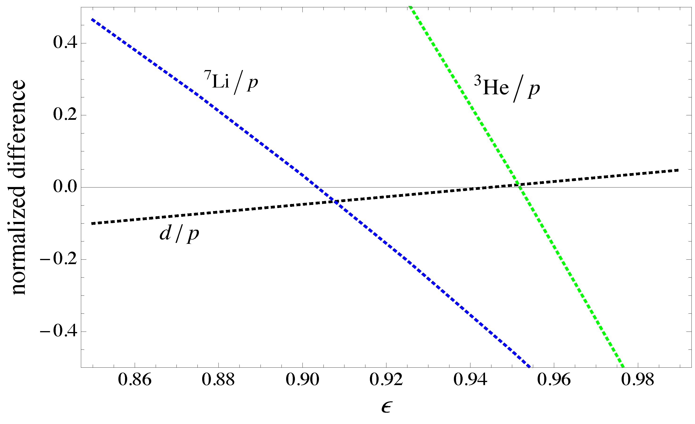
In Figure 7, we show the results of the simultaneous calculations for d, and , all normalized to p over the transition period. We have taken the observed nuclide ratios as , and (from Rich’s Figure 6.7 [4]). We then normalize the difference between our model ratios and the observed ratios by dividing by the observed ratios, as:
and varied the branching ratio ϵ to achieve a “best fit”. Our model under-predicts the ratio, but gives a good fit to the and ratio at a branching ratio . Clearly, Reaction (1) represents the dominant branch. We note that, if the astrophysical factor in the case of the reaction (7) was about a factor to two larger than that presented in the NACRE-II file (a possibility given the error bars at low energy in this reaction) or if the density was slightly larger, then this nuclide ratio would also come into agreement at .
Figure 7.
The normalized differences between the model and the observed nuclide ratios for in dotted black, the in dotted green and in dotted blue as a function of the branching ratio ϵ.
Figure 7.
The normalized differences between the model and the observed nuclide ratios for in dotted black, the in dotted green and in dotted blue as a function of the branching ratio ϵ.

The tresino nucleosynthesis reactions remove only a very small number of the p and that go on as rotors and PTMs in the expansion. Another important point to note is that the transition nucleosynthesis reactions are exothermic and might produce some observable heating and/or other collisional effects in the plasma flow.
Therefore, it appears that our high-density BB model along with tresino-mediated nucleosynthesis succeeds in reproducing the observed low-mass nuclide abundances (as does the SBBN), though it does so at a much later time.
7. The Phase Transition and the CMB
The cosmic microwave background radiation has been examined in detail in recent years, made possible by remarkable technological advances in microwave measurement capabilities, e.g., with WMAP. In particular, the distortions of the CMB radiation, within the standard model, has led to a methodology for precision data extraction from these observations. The standard model does not include our proposed phase transition, and to the extent that the transition affects the characteristics of the CMB (e.g., Section 6), it might have arrived at some inaccurate cosmological estimates, requiring re-examination. It is beyond the scope of this paper to attempt a detailed comparison of the CMB and its distortions incorporating the tresino phase transition. On the other hand, we will comment on a few specific effects that the phase transition might have on the CMB radiation.
The tresino phase transition takes place closer to the recombination era than the baryogenesis of the very early Universe. This implies potentially more influence upon the observations now, especially since the plasma composition in our model is considerably different than that of the standard model. Most important is the radiation from the spin-down of rotors into PTMs and the energy release by tresino nucleosynthesis. The PTMs would have little or no effect upon the plasma at recombination (except perhaps for some distortions), because they are both neutral and small. On the other hand, the fraction of the post-transition dark matter from rotors may contribute a large amount of radiation that continues on to and interacts with the recombination plasma. We note that the kinetic energies of some rotors may be as high as a keV/particle, because they have arisen from the kinetic recoil energies of the ejected tresino-proton pairs; lower energy rotors also contribute to photon generation, as shown in Section 5. The rotor spin-down photons, prior to recombination, will be rather low-energy; however, they are released into the plasma at a time when the ordinary plasma electrons are more energetic, so these photons may be up-scattered in Compton collisions and, at the same time, will cool the electron population (see Sunyaev and Zeldovich [20]). The effect of the radiation produced in rotor spin-down is probably small, but could, nonetheless, influence details of the CMB spectra. We note also that, due to the unique form of the energy from the phase transition, i.e., it appears as the kinetic energy of protons and tresinos, not as an increase in electron temperature, as are some suggested late-time energy sources (see [19]).
Some of the CMB distortions (associated with baryon oscillations in the primordial plasma) may have been induced in the post-transition plasma before the recombination era, that is at a much later time. The CMB radiation (and distortions) and its interactions from rotor spin-down, PTMs and ordinary matter recombination could be examined with a detailed non-adiabatic, non-equilibrium, multi-fluid, tresino transition dynamical model.
Finally, apart from possible particle and radiation effects, any magnetic fields that remain after the transition (see Section 8) may be present and would have to be examined for their effects on the CMB radiation.
Table 2 below summarizes the results of the tresino phase transition from the sections above.
| Parameter | Value |
|---|---|
| Normalized Hubble Constant | 0.71 |
| normalized mass | 1.0 |
| recombination | |
| Resonance Energy, | keV |
| Transition starts, | 103,000 |
| Temperature | 25 eV |
| Baryon Density | cm |
| Transition ends, | 88,000 |
| Dark Matter (PTMs), | 0.26 |
| Dark Matter (rotors), | 0.7 |
| ordinary matter | 0.04 |
| dark matter | 0.96 |
8. The Solar Corona
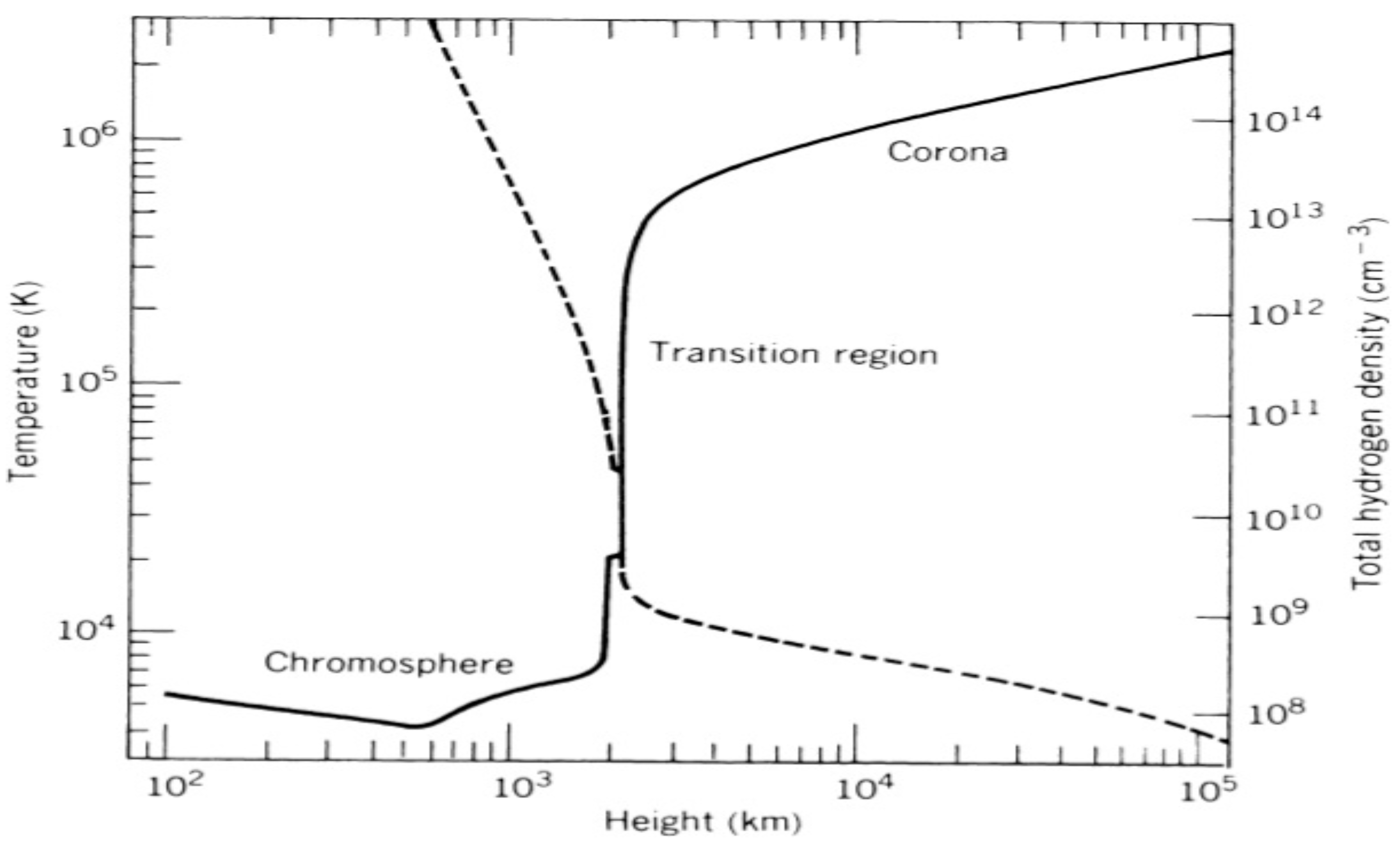
The source of heating in the solar corona has been a paradox for over fifty years (see Erdlyi and Ballai [21]). Looking at the densities and temperatures at the transition zone of the corona in Figure 8 (taken from Withbroe [22] (1981)), it is clear that these parameters are very close to those we obtain from the tresino phase transition late in the early Universe. Both the early Universe and the solar corona plasmas have evolved as the densities and temperatures have dropped, in expansion, from much higher values until both produce a tresino phase transition zone and an associated new source of energy. It is remarkable that the plateau density just outside of the corona transition zone is so close to the density (a few times ) where the tresino phase transition obtains in the early Universe. Withbroe [23] (1988) lists the required power flux into the corona at about 0.05 watts/cm and gives the electron density /cm and the flow velocity cm/s at the base of the corona. Multiplying by the tresino energy per transition (3.7 keV), the tresino transition power flux at this point is approximately 0.06 watts/cm; large enough to power additional heating of the corona. This estimate may be low, as the densities and velocities at the base of the corona are difficult to measure, as can be seen in Withbroe’s data. Still, the plasma streaming through the base of the corona is of the magnitude that is about right for a fraction of the electrons and protons to form ptres and then tresinos, releasing the binding energy to heat the corona, but only in this outer low-density zone. Of course, thermal conduction from this zone heats some of the plasma up-stream, at higher densities, as well. However, the primary heated zone is on the down-stream side of the corona’s transition zone.
Figure 8.
The solar corona density (dashed curve) and temperature (solid curve) plot taken from Withbroe (1981) [22].
Figure 8.
The solar corona density (dashed curve) and temperature (solid curve) plot taken from Withbroe (1981) [22].

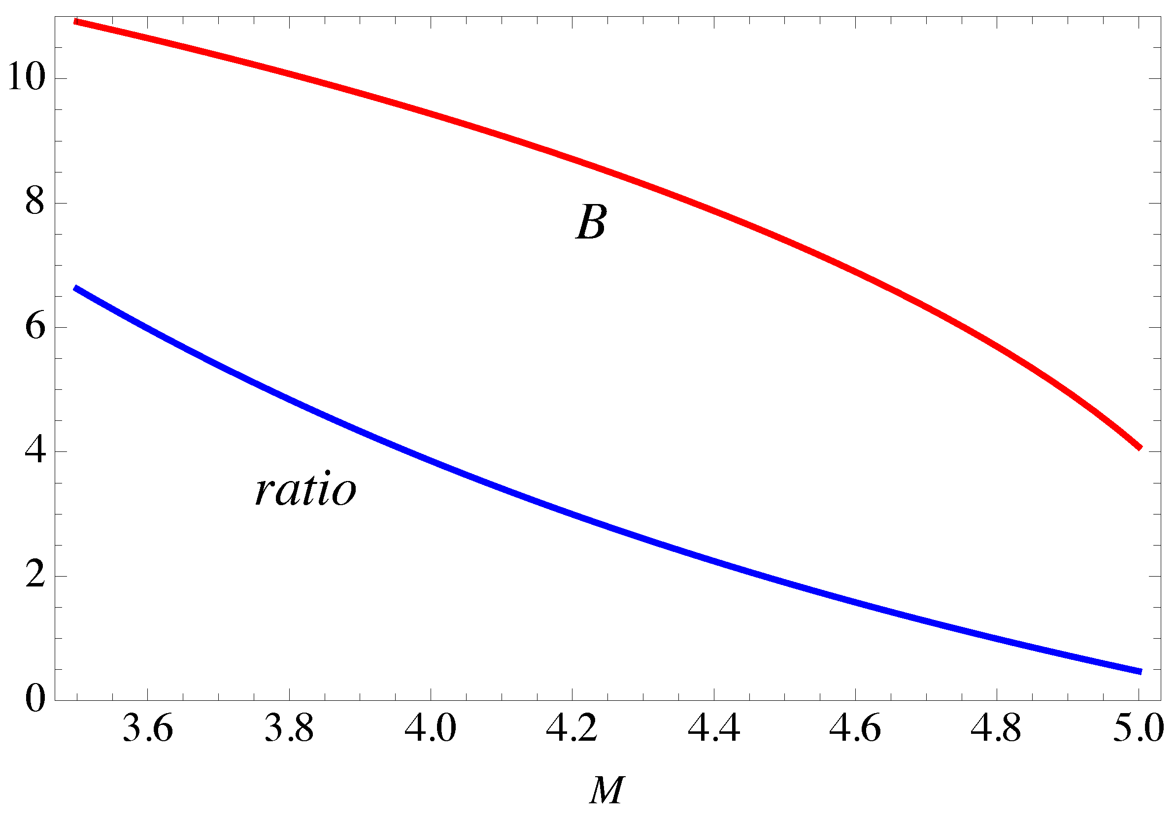
Now, let us examine the corona energy budget by writing down its components. The tresino energy density delivered to the base of the corona transition is ; the plasma energy (kinetic plus thermal energy) is ; the magnetic field energy is ; and finally, the gravitational potential energy having to be overcome is . Here, is the plasma density streaming out of the solar surface just before entering the corona; eV the Compton energy unit; is the (average) corona plasma temperature; M is a typical Mach number; and B is a typical magnetic field strength in the corona. In Figure 9, we display the numerical results for the magnetic field B and the ratio of the magnetic field energy density to the plasma energy density as a function of the Mach number, taking the number density /cm and eV. This simple one-zone model with the energy added by the tresino transition yields average values that are consistent with many solar corona measurements. It is interesting that a large fraction of the energy delivered from the tresino transition at intermediate Mach numbers (see Figure 9) appears as magnetic field energy, typically a factor of three more than the plasma energy. This observation suggests the interesting possibility that in the tresino transition late in the early Universe, some substantial amount of the expansion prior to the transition () can be found in the currents and magnetic fields produced after the transition. This fairly large amount of energy could be some fraction of the remainder of the early Universe expansion energy budget, i.e., the so-called dark energy. Magnetic energy has been proposed previously as a source of dark energy (see, for example, [24] and the references therein). However, these models appear to lack a basic source for their generation, whereas the tresino transition provides the charged particles, currents and fields in a straightforward way.
Finally, we note that the subject of magnetic fields at both interstellar and intergalactic scales has been difficult to understand from standard astrophysical and cosmological pictures (see Beck [25] and the references therein). Further, note that data extracted with the ΛCDM model predicts the dark energy density to be roughly equivalent to one proton/cm, equal to the magnetic energy density in an approximate 19 nanotesla field. The latter field strength is comparable to, or larger than, many astrophysical measurements (see the data in Beck). Hence, we conclude that the observations of the extraordinary magnetic activity in the solar corona might have been as likely during the tresino transition late in the early Universe as it appears to be in the solar corona today.
Figure 9.
The ratio of magnetic field energy to plasma energy and the magnetic field strength B (Gauss) in the corona as a function of the Mach number. See the text and Figure 8 for data.
Figure 9.
The ratio of magnetic field energy to plasma energy and the magnetic field strength B (Gauss) in the corona as a function of the Mach number. See the text and Figure 8 for data.

9. Discussion and Conclusions
We have proposed a new cosmological model that generates dark matter, not as relics from the very early Universe, but from Compton-scale composite structures composed of ordinary protons and electrons, late in the early Universe. Our model starts with, and maintains, a flat Universe throughout time and is consistent with most observations in cosmology and some in astrophysics. We do not invoke dark energy to make up the balance of the mass-energy of the Universe; in our picture, the energy resides in the mass of the rotors that have not had time to spin-down prior to recombination, as well as residual currents and magnetic field energy.
Our tresino transition cosmology will, of course, require re-examination in some areas of contemporary cosmology, such as the effects upon large-scale structure formation; it might have substantial differences when compared to the ΛCDM model. However, considering such changes now is beyond the scope of this paper. As previously mentioned, the tresino transition cosmology may have its own effects on the CMB, including the effects of the residual currents and magnetic fields at, and beyond, the recombination era.
Because the tresino phase transition releases rotor spin-down radiation before recombination, it may have its own distortions from interactions with the plasma before its release. In addition, we show in Appendix D that rotational modes of PTMs may be consistent with infrared spectral measurements in astrophysical observations at much later times.
Very late in the early Universe, our plasma composition is quite different from that of the standard model; it includes a small amount of ordinary matter, the CMB radiation, the PTMs, incompletely spun-down rotors and radiation, a residual low-density plasma of tresinos and protons possibly with currents and magnetic fields.
It is perhaps surprising that the tresino phase transition picture of dark matter generation may explain the origin of the heating of the solar corona with attendant currents and fields, through the same, but much later, phase transition conversion from ordinary to dark matter. If our picture of dark matter generation is correct, as mentioned, a number of cosmological estimates should be re-examined.
Ordinary matter stars appear to be embedded in halos of dark matter. This observation is to be expected if the coronae of the stars, like the Sun, are producing new dark matter driven by stellar winds into the surrounding interstellar regions. Tresinos can be ionized only if they encounter a very energetic environment, temperatures comparable to the binding energy of the tresinos, e.g., in the centers of hot stars or supernovae explosions; so, only in such environments can they be converted back into protons and electrons from whence they came. This re-transformation process is irreversible on short time-scales, so in this way, new ordinary matter may be re-created by the conversion of dark matter back into ordinary matter. Hence, a unique characteristic of these dark matter halos is their ability to be converted back into ordinary matter under special astrophysical situations by extracting energy from the environment, while continuing to be otherwise mostly hidden. However, the radiation from more recently excited PTM matter appears to be an indication of its presence in our time.
It is interesting that both ordinary and dark matter may be composed of the most common particles, electrons and protons, but with most of it in an uncommon electromagnetic configuration. Finally, if the coronae of stars are creating new dark matter, then the tresino phase transition may also be redistributing mass-energy in the expanding Universe, while conserving the net number of baryons.
Acknowledgments
The authors thank an earlier reviewer of this work for important criticisms, questions and suggestions. Frederick Mayer thanks Walter Fechner for helpful discussions.
Author Contributions
The work presented in this paper has evolved through a roughly twenty year collaboration between Frederick Mayer and John Reitz (see our recent publications); the theoretical developments of the tresino transition physics was done jointly. The transition equilibrium statistical mechanics (Appendix B) was mostly the work of John Reitz and the connection to the cosmological observations was mostly the work of Frederick Mayer.
Appendix A: A Simple ptre Model
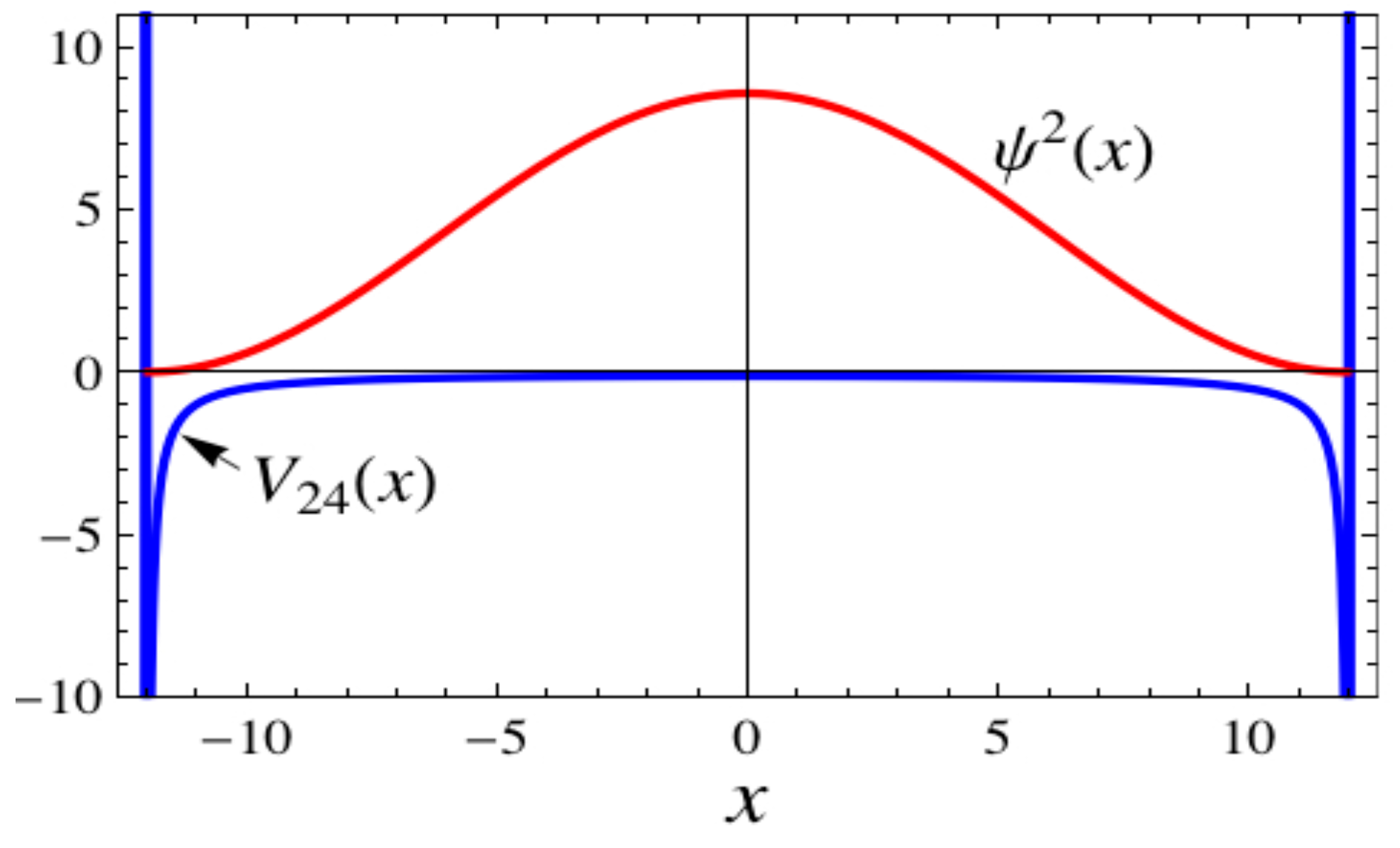
We present a simple model of the ptre as an Efimov scattering resonance. We consider the ptre as a linear three-body system, a formidable quantum mechanical problem, so we resort to a semi-classical model. We begin by calculating the classical electromagnetic forces and potentials of an electron captured between two protons a distance R apart, as in Figure 1b. We use a coordinate system where represents the electron’s position mid-way between the protons. The electron is attracted by both protons and repelled by the magnetic dipole-dipole force at each proton, sending the electron back toward the center. Of course, the spins must be correctly aligned, so as to repel the electron at both proton positions. It is straightforward to consider the classical problem of the electromagnetic forces on this linear three-body linear system and arrive at the potential given below:
with x the electron position, and is the electron’s magnetic moment and the proton’s magnetic moment. The Schrödinger equation for this linear “oscillator” may be written:
where α is the fine-structure constant, R and x are now measured in units and the energy eigenvalue and the potential are measured in Compton energy units (); notice that the potential is an even function of x. We take the distance between protons to be fixed, and therefore, there is a lowest energy eigenvalue for any particular value of R. The lowest energy states are readily found with numerical integration of this Schrödinger equation for a chosen value of R. A series of numerical integrations of the Schrödinger equation yields an approximate relation between the eigenvalue and the proton separation as . We consider the special case of with 3.7 keV and , i.e., the resonance energy is equal to one Compton energy unit. Figure A1 shows the potential and the wave-function (squared) for this special case. In examining a number of cases, we find that other choices for the resonance energy results in only slight changes in the location of the ptre phase transition (Section 3).
Figure A1.
Plot of red and potential blue with = 3.7 keV.

Appendix B: Saha–Boltzmann Equilibrium Combination
In order to find the temperature and density at which the ptres and tresinos will precipitate out of the cosmic plasma, we derive an equation similar to the Saha equation for the ionization of hydrogen atoms. We follow the procedure outlined by Weisstein [26] for the hydrogen recombination Saha equation and modify it for our problem. We set up a probability function for the particles involved and determine the most probable state. To simplify the notation, in the following, we denote the ptre by the abbreviated subscript .
For our problem, the basic relationship is:
and the probability function in Weisstein’s notation is:
where the Z’s are partition functions; e.g.,
where parameters have their usual definitions. Because of Equation (B1), we had to insert a second factor in Equation (B2). We take the spin of the ptre to be .
Now, let N be the total number of protons in the system, both in ptres and free protons:
Then,
Next, take the derivative of the with respect to and set the result to zero. The resulting relationship is:
and this can be rewritten as:
where is the total proton number density, and is the resonance scattering energy. Thus, Equation (B7) gives us the unbound electron fraction x as a function of temperature and density required in Section 3.
Finally, the equilibrium generation of the He or α-tresinos is easily derived from Equation (B7) by substituting for and setting keV. This shows that the more strongly bound α-tresinos come into equilibrium at a higher density, earlier in the expansion, than the p-tresinos. In the calculation, we start by choosing at the end of helium production (see Weinberg [3] page 166). We find that, after both the helium and hydrogen tresino transitions are complete, the helium to hydrogen ratio is about 1/3.
Appendix C: Rotors and PTMs As Dark Matter
As discussed in Section 5, the proton-tresino pairs will spin-down until their inter-particle distance is about 15 Comptons. If they have lost enough rotational energy, they will fall into a molecule-like composite, a proton-tresino molecule. Using the same physics that binds the tresino, electrostatic attraction at large distances and magnetic repulsion at short distances, it is possible to show that this energy binds the proton-tresino pair into a structure similar to, but not exactly the same as, a molecule, as shown in Figure 1c; we refer to these special molecules as PTMs. The binding energy of the PTMs is , where is the nominal distance between the tresino and proton. cannot be very much smaller than the radius of the tresino, which is roughly six Comptons. Hence, the PTM binding energy is on the order of a few hundred eV. A more precise value will have to await a more detailed (and difficult) theoretical analysis of the PTM structure; a subject that is beyond the scope of the present paper.
Let us now list some important points about PTMs. First, they are charge-neutral. Second, they are relatively robust with respect to particle collisions. Third, they will not aggregate like ordinary matter. Fourth, they are quite small, mobile and probably quick to thermalize in their environment. Finally, they have internal degrees of freedom, an aspect discussed in Appendix D. Because of the these characteristics, the PTMs may represent the pre-recombination era dark matter (see Section 5.4). We note some similar points about rotors. They are also charge-neutral at large distances and relatively robust with respect to particle collisions.
With these unique characteristics, we suggest that PTMs and incompletely spun-down rotors may be the mysterious and ubiquitous dark matter in the Universe.
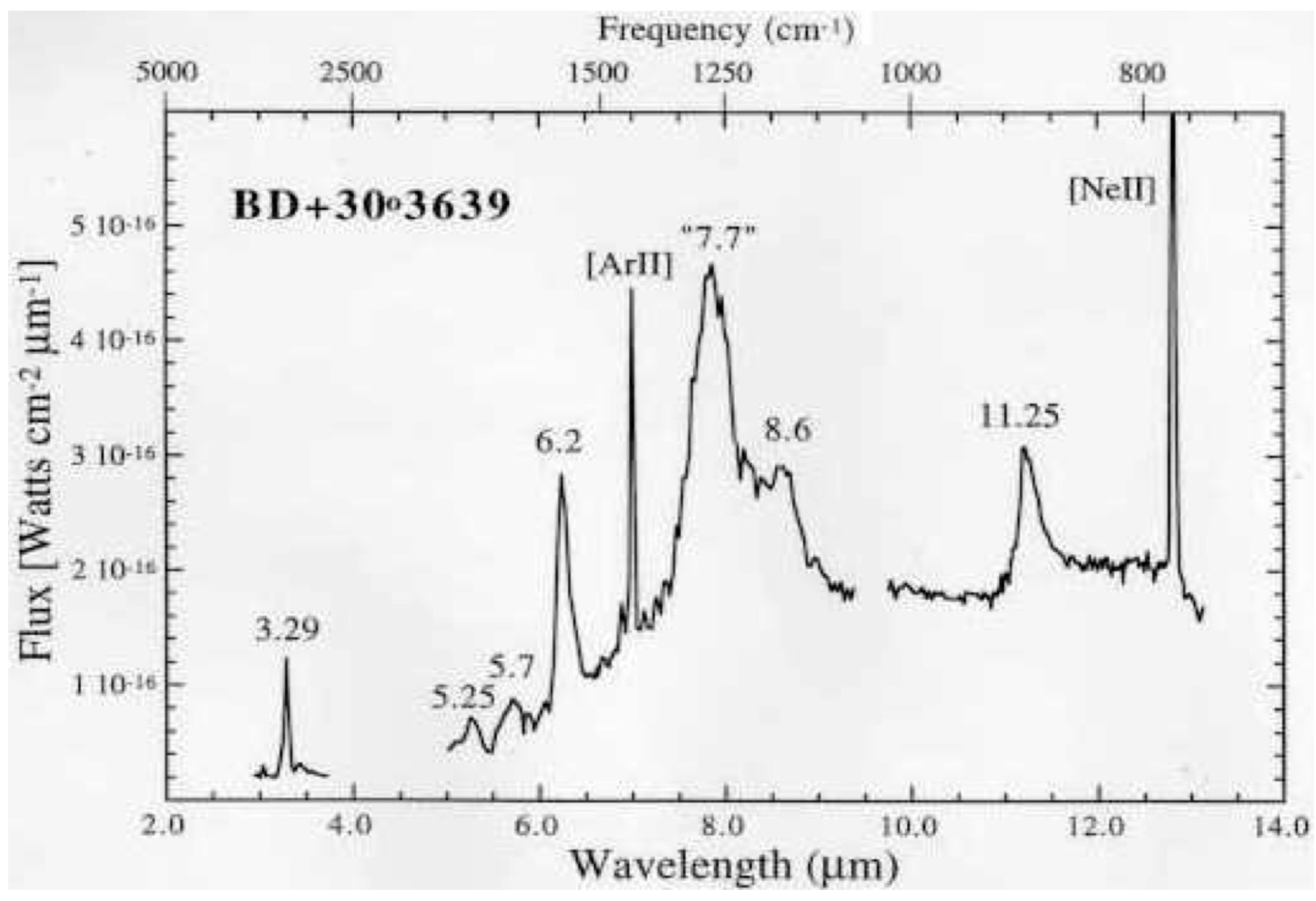
Appendix D: Cosmic Infrared Background
Long after the tresino phase transition is complete and after most tresinos and protons have combined, the Universe is composed of some rotors, some PTMs, a large amount of long-wavelength radiation and a small amount of ordinary matter. Both the rotors and PTMs can be “spun-up” by radiation from local energetic astrophysical sources and would be red-shifted, depending on their distance. Figure D1 (taken from a NASA website [27]) is an infrared spectrum that shows both continuum and line radiation. The rather strong infrared lines (earlier called “unidentified infrared bands” or UIBs) were discovered in the 1970s. The UIBs are ubiquitous and have been ascribed to certain polycyclic aromatic hydrocarbon molecules (PAHs) (Tielens [28], Lagache et al. [29]). The PAH molecules possess absorption and radiation in some appropriate infrared spectral regions. There are, however, some issues that make PAHs problematic. First, the PAHs would be readily evaporated in a high-temperature environment, whereas rotors and PTMs would not. Second, PAHs in the astrophysical environment would not be expected to be as ubiquitous as would be required for the UIBs. Finally, some studies have suggested that the amount of carbon required for the PAHs to be so plentiful is unrealistic.
We present an alternative picture, namely that the infrared line radiation is produced from “spun-up” rotors or PTMs, which make up a large fraction of the baryons in the Universe. Similar to conventional molecules, the PTMs are capable of both absorbing and emitting radiation characteristic of rigid-rotor quantized systems (more precisely, in the present case, a “non-rigid rotor”); a feature of their internal degrees of freedom. Rotors may be similarly excited and re-radiate energy, but they will have a different distribution of inter-particle dimensions; so for now, we will focus on the PTMs.
When a PTM finds itself in a high-temperature radiation environment, e.g., near a star, it may absorb energy from this field in a manner similar to well-known molecular rotational energy absorption and re-radiation in coherent series of rotational lines or bands. We will compare the PTMs to the observations of the UIBs.
We consider the simplest model for a diatomic non-rigid rotor calculation. At higher angular momentums (larger Js), there is a correction that takes account of the change in the moment of inertia of a rigid-rotor model. The energy levels are given by (see, e.g., Harmony [30]):
where and and are the proton mass and the average tresino-proton separation, respectively. The second term in Equation (D1) is the centrifugal stretching correction to the rigid rotor; it is generally small. The third term in Equation (D1) is a correction for either a prolate or oblate spheroid; we neglect this term. In the calculations, the second term will be treated as the parameter .
Figure D1.
Infrared spectrum with unidentified infrared bands; courtesy of NASA.

Table D1 shows the comparison between the UIB lines and our rotor model calculation, where the best fit had Comptons and . As can be seen, the agreement is fairly close, but not perfect. The strong line at 7.7 μm may be a result of the PTMs prolate shape adding additional vibrational modes. Requiring the third term in Equation (D1), where K takes on the values , will both increase the strength and broaden this line. This exercise in data fitting does not confirm the PTMs as a component of dark matter, but it does make it more plausible.
| UIB lines | 11.25 | 8.6 | 7.7 | 6.2 | 3.29 |
|---|---|---|---|---|---|
| Rotor lines | 11.17 | 8.83 | see text | 6.11 | 3.12 |
In a similar manner, for those rotors that have not had time to completely spin-down and become PTMs, there will be comparable absorption and re-radiation, due to spin-up, but they would be, of course, at different wavelengths.
Conflicts of Interest
The authors declare no conflicts of interest.
References
- Schramm, D.; Turner, M. Big-bang Nucleosynthesis enters the Precision Era. Rev. Mod. Phys. 1998, 70, 303–318. [Google Scholar] [CrossRef]
- Kolb, E.; Turner, M. The Early Universe (Frontiers in Physics) 69; Addison-Wesley: Redwood City, CA, USA, 1990. [Google Scholar]
- Weinberg, S. Cosmology; Oxford University Press: Oxford, UK, 2008. [Google Scholar]
- Rich, J. Fundamentals of Cosmology; Springer-Verlag: Berlin, Germany, 2009. [Google Scholar]
- Mayer, F.; Reitz, J. Electromagnetic Composites at the Compton Scale. Int. J. Theor. Phys. 2012, 51, 322–330. [Google Scholar] [CrossRef]
- Efimov, V. Energy levels arising from resonant two-body forces in a three-body system. Phys. Lett. B 1970, 33, 563–564. [Google Scholar] [CrossRef]
- Kraemer, T.; Mark, M.; Waldburger, P.; Danzl, J.G.; Chin, C.; Engeser, B.; Lange, A.D.; Pilch, K.; Jaakkola, A.; Ngerl, H.-C.; et al. Evidence for Efimov quantum states in an ultracold gas of caesium atoms. Nature 2006, 440, 315–318. [Google Scholar] [CrossRef] [PubMed]
- Nishida, Y.; Son, D.T.; Tan, S. Universal fermi gas with two- and three-body resonances. Phys. Rev. Lett. 2008, 100. [Google Scholar] [CrossRef]
- Mayer, F.; Reitz, J. Thermal Energy Generation in the Earth. Nonlinear Process. Geophys. 2014, 21, 367–378. [Google Scholar] [CrossRef]
- Jarosik, N.; Bennett, C.L.; Dunkley, J.; Gold, B.; Greason, M.R.; Halpern, M.; Hill, R.S.; Hinshaw, G.; Kogut, A.; Komatsu, E.; et al. Seven-Year Wilkinson Microwave Anisotropy Probe (WMAP) Observations: Sky Maps, Systematic Errors, and Basic Results. ArXiv E-Prints 2010. arXiv:1001.4744. [Google Scholar]
- Marion, J.B.; Heald, M.A. Classical Electromagnetic Radiation, 2nd ed.; Academic Press: New York, NY, USA, 1980. [Google Scholar]
- Kogut, A. Synchrotron Spectral Curvature from 22 MHz to 23 GHz. ArXiv E-Prints 2012. arXiv:1205.4041. [Google Scholar] [CrossRef]
- Strong, A.W.; Orlando, E.; Jaffe, T.R. The interstellar cosmic-ray electron spectrum from synchrotron radiation and direct measurements. Astron. Astrophys. 2011, 534, A54. [Google Scholar] [CrossRef]
- Riess, A.G.; Filippenko, A.V.; Challis, P.; Clocchiattia, A.; Diercks, A.; Garnavich, P.M.; Gilliland, R.L.; Hogan, C.J.; Jha, S.; Kirshn, R.P.; et al. Observational Evidence from Supernovae for an Accelerating Universe and a Cosmological Constant. Astron. J. 1998, 116, 1009–1038. [Google Scholar] [CrossRef]
- Perlmutter, S.; Aldering, G.; Goldhaber, G.; Knop, R.A.; Nugent, P.; Castro, P.G.; Deustua, S.; Fabbro, S.; Goobar, A.; Groom, D.E.; et al. Measurements of Ω and Λ from 42 High-Redshift Supernovae. Astrophys. J. 1999, 517, 565–586. [Google Scholar] [CrossRef]
- Landau, L.D.; Lifshitz, E.M. Quantum Mechanics—Non-Relativistic Theory; Addison-Wesley Publishing Company: Boston, MA, USA, 1958. [Google Scholar]
- Rolfs, C.E.; Rodney, W.S. Cauldrons in the Cosmos; University of Chicago Press: Chicago, IL, USA, 1988; Chapter 6. [Google Scholar]
- Knapp, G. The Physics of Fusion in Stars. Available online: http://www.astro.princeton.edu/gk/A403/fusion (accessed on 17 May 2014).
- NACRE II Nuclear Reaction Data. Available online: http://www.astro.ulb.ac.be/nacreii/ (accessed on 7 July 2014).
- Sunyaev, R.A.; Zel’dovich, Y.B. Microwave Background Radiation as a Probe of the Contemporary Structure and History of the Universe. Annu. Rev. Astron. Astrophys. 1980, 18, 537–560. [Google Scholar] [CrossRef]
- Erdelyi, R.; Ballai, I. Heating of the solar and stellar coronae: A review. Astron. Nachr. 2007, 328, 726–733. [Google Scholar] [CrossRef]
- Withbroe, G. Activity and Outer Atmospheres of the Sun and Stars; 11th Advanced Course; Swiss Society of Astronomy and Astrophysics (SAAS-FEE): Bern, Switzerland, 1981. [Google Scholar]
- Withbroe, G.L. The temperature structure, mass, and energy flow in the corona and inner solar wind. Astrophys. J. 1988, 325, 442–467. [Google Scholar] [CrossRef]
- Contopoulos, I.; Basilakos, S. The tension of cosmological magnetic fields as a contribution to dark energy. Astron. Astrophys. 2007, 471, 59–63. [Google Scholar] [CrossRef]
- Beck, R. Galactic and extragalactic magnetic fields—A concise review. Astrophys. Space Sci. Trans. 2009, 5, 43–47. [Google Scholar] [CrossRef]
- Weisstein, E. Eric Weisstein’s World of Physics. 2006. Available online: http://www.physics.utah.edu/ kieda/SahaEquation (accessed on 26 September 2006).
- The National Aeronautics and Space Administration (NASA). Available online: http://map.gsfc.nasa.gov/Universe/uni-matter.html (accessed on 12 February 2010).
- Tielens, A. Interstellar polycyclic hydrocarbon molecules. Annu. Rev. Astron. Astrophys. 2008, 46, 289–337. [Google Scholar] [CrossRef]
- Lagache, G.; Puget, J.-L.; Dole, H. Dusty Infrared Galaxies: Sources of the Cosmic Infrared Background. Annu. Rev. Astron. Astrophys. 2005, 43, 727–768. [Google Scholar] [CrossRef]
- Harmony, M. Molecular Spectroscopy and Structure. In Physics Vade Mecum; Anderson, H.L., Ed.; American Institute of Physics: New York, NY, USA, 1981; p. 222. [Google Scholar]
© 2014 by the authors; licensee MDPI, Basel, Switzerland. This article is an open access article distributed under the terms and conditions of the Creative Commons Attribution license (http://creativecommons.org/licenses/by/3.0/).
Share and Cite
MDPI and ACS Style
Mayer, F.; Reitz, J. Compton Composites Late in the Early Universe. Galaxies 2014, 2, 382-409. https://doi.org/10.3390/galaxies2030382
AMA Style
Mayer F, Reitz J. Compton Composites Late in the Early Universe. Galaxies. 2014; 2(3):382-409. https://doi.org/10.3390/galaxies2030382
Chicago/Turabian StyleMayer, Frederick, and John Reitz. 2014. "Compton Composites Late in the Early Universe" Galaxies 2, no. 3: 382-409. https://doi.org/10.3390/galaxies2030382