Constraints on Non-Standard Gravitomagnetism by the Anomalous Perihelion Precession of the Planets

Abstract

In 2008, a team of astronomers reported an anomalous retrograde precession of the perihelion of Saturn amounting to $\Delta {\dot{\omega }}_{\text{S}}$_aturn = −0.006(2) arcsec per century (arcsec cy⁻¹). This unexplained precession was obtained after taking into account all classical and relativistic effects in the context of the highly refined EPM2008 ephemerides. More recent analyzes have not confirmed this effect, but they have found similar discrepancies in other planets. Our objective in this paper is to discuss a non-standard model involving transversal gravitomagnetism generated by the Sun as a possible source of these potential anomalies, to be confirmed by further data analyses. In order to compute the Lense–Thirring perturbations induced by the suggested interaction, we should consider the orientation of the Sun’s rotational axis in Carrington elements and the inclination of the planetary orbits with respect to the ecliptic plane. We find that an extra component of the gravitomagnetic field not predicted by General Relativity could explain the reported anomalies without conflicting with the Gravity Probe B experiment and the orbits of the geodynamics satellites.

1. Introduction

The residual anomalous advance of the perihelion of Mercury was a keystone experimental fact in the early development of the General Theory of Relativity. Nowadays many tests have been performed, and all of them are in agreement with the predictions of the theory within the experimental precision [1]. Nevertheless, the accuracy of astronomical observations is constantly increasing thanks to the development of new techniques, such as radar and laser ranging and tracking of spacecraft and planets. To the list of unexplained anomalies, we can add the secular increases of the astronomical unit and the eccentricity of the orbit of the Moon [2]. Some attempts based upon non-standard physics have recently been discussed in the literature [3,4,5,6], and also, many conventional explanations have been considered and dismissed [7,8,9,10]. Another celestial mechanics anomaly repeatedly confirmed in several data analyzes is the secular change of the Sun’s gravitational parameter Gravitational Constant times the Mass of the Sun ($GM$) [11,12,13,14]. However, we cannot exclude the possibility that further investigations could show that these anomalies are not statistically significant.

Another issue in the celestial mechanics of the Solar System, which have been found and discussed in the last few years, is an anomalous extra retrograde precession of the perihelion of Saturn unmodeled by classical and relativistic effects [15,16]. This retrograde precession is very small, $\Delta {\dot{\omega }}_{\text{S}}$_aturn = − 0.006 (2) arcsec per century, but still different from zero at the $3\sigma$ level.

This unexpected result was found by Pitjeva after processing a very large data set of planetary data covering the period from 1913 to 2007 and using the high accuracy ephemerides model to that date: EPM2008 [15,17]. The precision of the analysis is exquisite, because it includes the action of trans-Neptunian dwarf planets, such as Eris, other 20 trans-Neptunian objects, the solar quadrupole, the individual actions of the 301 biggest asteroids and a massive ring for the smaller ones, as well as the corrections induced by General Relativity. However, these results have not been confirmed by other authors [18], and the EPM2011 model used by Pitjeva does not find the anomaly for Saturn within the error bars, but gives non-zero values for the supplementary precession of Jupiter and Venus [13]. The EPM2013 ephemerides model is now available [12], although no extra precessions of the perihelia are included.

Unfortunately, the accuracy is still not sufficient to claim a similar effect on the other planets, and the errors are still very high to achieve any definitive conclusion. However, if this extra precession is finally confirmed, it should pose an important challenge to our understanding of gravity. As Iorio pointed out [15], an extra precession of orbits is predicted by the Dvali–Gabadadze–Porrati multidimensional braneworld scenario [19,20], as shown by Lue and Starkman [21], but this is very small, $\simeq \pm 0.0005$ milliarcsec per century, in comparison with the observation for Saturn’s orbit. Another possible origin could be the presence of a spherically symmetric dark matter halo inside the Solar system, as suggested by Khriplovich and Pitjeva [22], and the effect has been used to set upper limits on the amount of dark matter bound to the Sun [23]. MONDtheory with different parameters is another alternative [24], but the predicted extra orbital precession is out of range [15]. The estimated corrections $\Delta \dot{\omega }$ to the anomalous Newton/Einstein perihelion precession of the inner planets have also been used to find bounds on a possible secular variation of the speed of light [25]. The existence of an undiscovered large trans-Neptunian planet or even a dwarf star, moving in a highly elliptic orbit around the Sun [26,27,28,29,30,31,32,33,34], is another possibility proposed as an explanation of the anomaly in the orbit of Saturn. A retrograde precession, adding to the General Relativity prediction for the movement of Saturn in the Schwarzschild’s spacetime around the Sun, is originated by the gravitomagnetic field generated by the rotation of the Sun [35,36,37]. However, this effect is very small at Saturn’s distance, and it is estimated as $-{10}^{-7}$ milliarcsec/cy, i.e., four orders of magnitude below the reported anomaly. The gravitomagnetic field [38] for a rotating star takes the form:

$${\displaystyle \mathbf{B}=-\frac{1}{5}\frac{r_S}{r}{\left({\displaystyle \frac{R}{r}}\right)}^2\left[W-3\left(W·\widehat{\mathbf{r}}\right)\widehat{\mathbf{r}}\right]}$$

(1)

where $r_S=2GM/c^2$ is the Schwarzschild radius of the body, R is the Sun’s radius and W is the angular velocity vector. This field gives rise to a small acceleration of the planets given by a Lorentz force law:

$${\displaystyle \mathbf{a}=-\frac{2}{c}\mathbf{v}\times \mathbf{B}}$$

(2)

and this expression justifies the denomination of $\mathbf{B}$ as a gravitomagnetic field. The force lines of the field in Equation (1) can be interpreted classically as a dipolar field generated by the angular momentum of the rotating body, in a similar fashion to the magnetic field of a rotating charged sphere. It has been pointed out that the Gravity Probe B experiment, despite its high accuracy, does not preclude the existence of a putative transversal gravitomagnetic component of the field generated by the rotating Earth [39]. This component does not accumulate as a secular effect in the orientation of the on-board gyroscopes, and consequently, it could remain hidden. Of course, this field could only arise in a modified theory of gravity, because it is not predicted by conventional General Relativity. We will not speculate in this paper about the necessary modification giving rise to this new effect, which may include, for example, torsion or nonsymmetric fields [40,41], but we should proceed phenomenologically by proposing:

$${\displaystyle {\mathbf{B}}_{n,m}(r,\theta )=B(r,\theta )\widehat{\varphi }=\beta W\frac{r_S}{r}{sin}^n\theta {cos}^m\theta \widehat{\varphi },n=1,2,\dots ,m=0,1,\dots .}$$

(3)

where $\widehat{\varphi }$ is the azimuthal unit vector, θ is the polar angle and β is a constant to be determined. The integer $n\ge 1$ because $B(r,\theta =0)=B(r,\theta =\pi )=0$ for continuity reasons. In this paper, we study the effect of a gravitomagnetic field of this kind on the perihelion advance of planetary orbits. We will show that, depending on the relative orientation of the Sun axis and the planet’s orbital plane, prograde and retrograde precession effects are found.

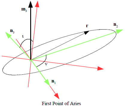
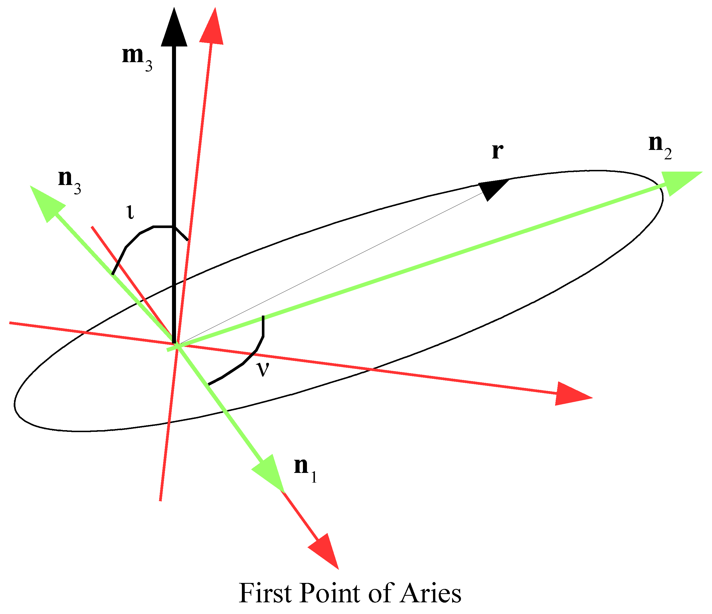
2. Definitions and Orbital Data

The calculation of the perturbation effect by the field in Equation (3) requires some orbital and the Sun’s rotation parameters. The orientation of the axis of the Sun with respect to the ecliptic plane is given by the so-called Carrington’s elements [42] as follows:

$$\begin{array}{ccc}\hfill {\iota }_c& =& 7.{25}^{\circ }\hfill \end{array}$$

(4)

$$\begin{array}{ccc}\hfill {\Omega }_c& =& 73.{67}^{\circ }+0.{013958}^{\circ }(t-1850)\hfill \end{array}$$

(5)

where ${\iota }_c$ is the inclination of the Sun’s rotational axis, ${\Omega }_c$ is the longitude of the ascending node corresponding to the equatorial plane of the Sun and t is the year of observation; this second term corresponds to the slow precession of the Sun’s rotational axis with time. Both angles are measured in degrees. Similarly, the rotation plane of a planet is defined by two vectors: one of them aligned with the first point of Aries and the other one along the inclination vector for that orbit. In terms of the inclination angle, ι, and the longitude of the ascending node, Ω, we have:

$$\begin{array}{ccc}\hfill {\widehat{\mathbf{n}}}_1& =& cos\Omega \widehat{ı}+sin\Omega \widehat{j}\hfill \end{array}$$

(6)

$$\begin{array}{ccc}\hfill {\widehat{\mathbf{n}}}_2& =& -cos\iota sin\Omega \widehat{ı}-sin\iota cos\Omega \widehat{j}+cos\iota \widehat{k}\hfill \end{array}$$

(7)

$$\begin{array}{ccc}\hfill {\widehat{\mathbf{n}}}_3& =& sin\iota sin\Omega \widehat{ı}-sin\iota cos\Omega \widehat{j}+cos\iota \widehat{k}\hfill \end{array}$$

(8)

This is an orthonormal reference system for the orbit. In this orbital system, we have the following relations for the orbital radius vector and velocity [43,44]:

$$\begin{array}{ccc}\hfill \mathbf{r}& =& {\displaystyle p\frac{cos\nu {\widehat{\mathbf{n}}}_1+sin\nu \widehat{{\mathbf{n}}_2}}{1+ϵcos(\nu -\omega )}}\hfill \end{array}$$

(9)

$$\begin{array}{ccc}\hfill \mathbf{v}& =& \sqrt{{\displaystyle \frac{\mu }{p}}}\left\{-(sin\nu +ϵsin\omega ){\widehat{\mathbf{n}}}_1+(cos\nu +ϵcos\omega ){\widehat{\mathbf{n}}}_2\right\}\hfill \end{array}$$

(10)

$p=a(1-{ϵ}^2)$ being the semilatus rectum, a is the semi-major axis, ϵ the orbital eccentricity, ν the true anomaly, ω the longitude of the perihelion and $\mu =GM$ is the product of the gravitational constant and the Sun’s mass. In our definition, the true anomaly is the angle among the position vector of the planet and the ascending node. Notice that, usually, the true anomaly is measured from the perihelion. A picture of a typical orbit and the corresponding vectors defining its system of reference is shown in Figure 1. From the relations in Equation (9) and the orientation angles for the Sun’s rotation axis in Equation (4), we calculate the unit vectors ${\widehat{\mathbf{m}}}_i$, $i=1,2,3$, which constitute another system of reference anchored to the Sun. It is also useful to define the matrix:

$${\alpha }_{ij}={\widehat{\mathbf{n}}}_i·{\widehat{\mathbf{m}}}_j$$

(11)

As in Equation (3), the polar and azimuthal angles, θ and ϕ, appear explicitly, we must relate them to the orbital parameters in order to analyze the perturbation effects. These angles correspond to a spherical coordinate system in which the z-axis is the rotation axis of the Sun. Therefore, we can write:

$${\displaystyle cos\theta =\frac{\mathbf{r}}{r}·{\widehat{\mathbf{m}}}_3={\alpha }_{13}cos\nu +{\alpha }_{23}sin\nu }$$

(12)

which gives us the cosine of the polar angle in terms of the true anomaly of the planet. A similar relation is found for the azimuthal angle:

$$\begin{array}{ccc}\hfill cos\varphi & =& {\displaystyle \frac{{\alpha }_{11}cos\nu +{\alpha }_{21}sin\nu }{\sqrt{1-{({\alpha }_{13}cos\nu +{\alpha }_{23}sin\nu )}^2}}}\hfill \end{array}$$

(13)

$$\begin{array}{ccc}\hfill sin\varphi & =& {\displaystyle \frac{{\alpha }_{12}cos\nu +{\alpha }_{22}sin\nu }{\sqrt{1-{({\alpha }_{13}cos\nu +{\alpha }_{23}sin\nu )}^2}}}\hfill \end{array}$$

(14)

The azimuthal unit vector is also given by:

$$\widehat{\varphi }=-sin\varphi {\widehat{\mathbf{m}}}_1+cos\varphi {\widehat{\mathbf{m}}}_2$$

(15)

Figure 1. The relative orientation of the reference systems used in the calculations is as follows: the orthogonal system of reference corresponding to the ecliptic plane is shown in red; the system of a typical planetary orbit (${\widehat{\mathbf{n}}}_i$, $i=1$, 2, 3) in green; and the rotational axis of the Sun is ${\widehat{\mathbf{m}}}_3$. The true anomaly, ν, is the angle between the planet’s radius vector and the line of nodes (which in this plot coincides with the line pointing towards the first point of Aries). The inclination angle, ι, of the orbital plane is also displayed.

Figure 1. The relative orientation of the reference systems used in the calculations is as follows: the orthogonal system of reference corresponding to the ecliptic plane is shown in red; the system of a typical planetary orbit (${\widehat{\mathbf{n}}}_i$, $i=1$, 2, 3) in green; and the rotational axis of the Sun is ${\widehat{\mathbf{m}}}_3$. The true anomaly, ν, is the angle between the planet’s radius vector and the line of nodes (which in this plot coincides with the line pointing towards the first point of Aries). The inclination angle, ι, of the orbital plane is also displayed.

From Equations (3), (6) and (15), we can explicitly compute the perturbation force arising from the transversal gravitomagnetic field:

$$\delta \mathbf{F}=B(r,\theta )\widehat{\mathbf{v}}\times \widehat{\varphi }$$

(16)

It is clear that this perturbation does not change the total energy, because it is always perpendicular to the velocity, but the orbital angular momentum (per unit mass) should change according to:

$${\displaystyle \frac{d\mathbf{H}}{dt}=\mathbf{r}\times \delta \mathbf{F}=B(r,\theta )\mathbf{r}\times \left(\mathbf{v}\times \widehat{\varphi }\right)}$$

(17)

If we perform the dot product of both members of Equation (17) by $\mathbf{H}$, the following equation for the evolution of the angular momentum modulus is found:

$${\displaystyle \frac{1}{2}\frac{d{H}^2}{dt}=B(r,\theta )\left(\mathbf{r}\times \mathbf{v}\right)·\left\{\mathbf{r}\times \left(\mathbf{v}\times \widehat{\varphi }\right)\right\}}$$

(18)

In order to simplify the dot product, we use the Binet–Cauchy identity and the permutation of the scalar triple product [45] as follows:

$$\begin{array}{ccc}\hfill \left(\mathbf{r}\times \mathbf{v}\right)·\left\{\mathbf{r}\times \left(\mathbf{v}\times \widehat{\varphi }\right)\right\}& =& r^2\mathbf{v}·\left(\mathbf{v}\times \widehat{\varphi }\right)-\mathbf{r}·\left(\mathbf{v}\times \widehat{\varphi }\right)\left(\mathbf{r}·\mathbf{v}\right)\hfill \\ \hfill & =& -\left(\widehat{\varphi }·\mathbf{H}\right)\left(\mathbf{r}·\mathbf{v}\right)\hfill \end{array}$$

(19)

2.1. Components of the Perturbation Force

From Equations (18) and (19), we finally get:

$${\displaystyle \frac{dH}{dt}=-\left(\mathbf{r}·\mathbf{v}\right)\left(\widehat{\varphi }·{\widehat{\mathbf{n}}}_3\right)B(r,\theta )}$$

(20)

where ${\widehat{\mathbf{n}}}_3$ is the unit vector normal to the planetary orbit. Now, the tangential component of the perturbation force acting upon the planet can be deduced from Equations (9), (11), (15) and (20) as follows:

$${\displaystyle \mathcal{T}=\frac{1}{r}\frac{dH}{dt}=-ϵ\sqrt{{\displaystyle \frac{\mu }{p}}}sin\left(\nu -\omega \right)B(r,\theta )\left\{{\displaystyle \frac{\left({\alpha }_{11}{\alpha }_{32}-{\alpha }_{12}{\alpha }_{31}\right)cos\nu +\left({\alpha }_{21}{\alpha }_{32}-{\alpha }_{22}{\alpha }_{31}\right)sin\nu }{sin\theta }}\right\}}$$

(21)

where the expression for the intensity of the gravitomagnetic field was given in Equation (3) and the polar angle can be related to the true planetary anomaly by Equation (12).

The aforementioned condition for the conservation of the total energy implies the following relation among the radial and tangential components of the force:

$${\displaystyle \frac{dE}{dt}=\mathcal{R}\frac{dr}{dt}+r\mathcal{T}\frac{d\theta }{dt}=0}$$

(22)

or, equivalently:

$${\displaystyle \mathcal{R}=-r\frac{d\theta }{dr}\mathcal{T}=-\frac{1+ϵcos\left(\nu -\omega \right)}{ϵsin\left(\nu -\omega \right)}\mathcal{T}}$$

(23)

The component normal to the orbit, $\mathcal{N}$, is finally obtained as the scalar product:

$$\begin{array}{ccc}\hfill \mathcal{N}& =& \delta \mathbf{F}·{\widehat{\mathbf{n}}}_3=B(r,\theta )\widehat{\varphi }·\left({\widehat{\mathbf{n}}}_3\times \mathbf{v}\right)\hfill \\ & =& {\displaystyle -\sqrt{{\displaystyle \frac{\mu }{p}}}B(r,\theta )\left\{-sin\varphi (sin\nu +ϵsin\omega ){\alpha }_{21}-sin\varphi (cos\nu +ϵcos\omega ){\alpha }_{11}\right.}+\left.cos\varphi (sin\nu +ϵsin\omega ){\alpha }_{22}+cos\varphi \left(cos\nu +ϵcos\omega \right){\alpha }_{12}\right\}\hfill \end{array}$$

(24)

3. Results and Discussion

From the discussion of the previous section, we have found expressions for the radial, tangential and normal components of the perturbing force arising from the gravitomagnetic field in Equation (3). The secular precession of the perihelion can be now found from the classical equations from perturbation theory as follows [43,44]:

$$\begin{array}{ccc}\hfill {\displaystyle \frac{d\omega }{dt}}& =& {\displaystyle \sqrt{{\displaystyle \frac{p}{\mu }}}\frac{1}{ϵ}\left[{\displaystyle \frac{\left(2+ϵcos(\nu -\omega )\right)sin(\nu -\omega )}{1+ϵcos(\nu -\omega )}\mathcal{T}}\right.}\hfill \\ \hfill & & -\left.{\displaystyle \mathcal{R}cos(\nu -\omega )-\frac{ϵ}{1+ϵcos(\nu -\omega )}cot\iota sin\nu \mathcal{N}}\right]\hfill \end{array}$$

(25)

where $\mathcal{R}$, $\mathcal{T}$ and $\mathcal{N}$ are given by Equations (21), (23) and (24), respectively. The secular increase of the argument of the perihelion per unit time is obtained as the average of Equation (25) over the period $2\pi$ of the true anomaly, ν. In order to perform these calculations explicitly, we require the values for the relevant planetary elements [46] as listed in Table 1. The standard relation between time, t, and the eccentric anomaly of the planet, η [43,44], can be rewritten in terms of the true anomaly as follows:

$$\begin{array}{ccc}\hfill dt& =& {\displaystyle \frac{P}{2\pi }\left(1-cos\eta \right)d\eta }\hfill \\ \hfill & =& {\displaystyle \frac{P}{2\pi }\frac{{\left(1-{ϵ}^2\right)}^{3/2}}{{\left(1+ϵcos(\nu -\omega )\right)}^2}d\nu }\hfill \end{array}$$

(26)

We can now find the instantaneous derivative of the argument of the perihelion with respect to the true anomaly:

$${\displaystyle \frac{d\omega }{d\nu }=\frac{P}{2\pi }\frac{{\left(1-{ϵ}^2\right)}^{3/2}}{{\left(1+ϵcos(\nu -\omega )\right)}^2}\frac{d\omega }{dt}}$$

(27)

and the integral of this expression in the interval $0\le \nu \le 2\pi$ should give us the advance of the perihelion in a single orbit.

Table 1. Orbital elements of the planets: a: Semi-major axis; ϵ: orbital eccentricity; ω: argument of the perihelion; Ω: longitude of the ascending node; and ι: inclination of the orbital plane with respect to the ecliptic plane. All angles are given in sexagesimal degrees.

Planet	a (km)	ϵ	ω	Ω	ι
Mercury	57,909,100	0.205630	29.124°	48.331°	7.005°
Venus	108,208,000	0.00677323	55.186°	76.678°	3.394°
Earth	149,598,261	0.01671123	114.208°	−11.260°	1.579°
Mars	227,939,100	0.093315	286.537°	49.562°	1.850°
Jupiter	778,547,200	0.048775	275.066°	100.492°	1.305°
Saturn	1,433,449,370	0.055723219	336.014°	113.643°	2.485°

Table 1. Orbital elements of the planets: a: Semi-major axis; ϵ: orbital eccentricity; ω: argument of the perihelion; Ω: longitude of the ascending node; and ι: inclination of the orbital plane with respect to the ecliptic plane. All angles are given in sexagesimal degrees.

Planet	a (km)	ϵ	ω	Ω	ι
Mercury	57,909,100	0.205630	29.124°	48.331°	7.005°
Venus	108,208,000	0.00677323	55.186°	76.678°	3.394°
Earth	149,598,261	0.01671123	114.208°	−11.260°	1.579°
Mars	227,939,100	0.093315	286.537°	49.562°	1.850°
Jupiter	778,547,200	0.048775	275.066°	100.492°	1.305°
Saturn	1,433,449,370	0.055723219	336.014°	113.643°	2.485°

The instantaneous derivative as given by Equation (27) for a gravitomagnetic law with $n=m=2$ and $\beta =1$ has been plotted for the orbit of Saturn in Figure 2.

We should calculate the values by performing the average of the perihelion precession over a whole period, $\Delta \dot{\omega }$, for the inner planets, Jupiter and Saturn by using the data in Table 1. These values are listed in Table 2 for several pairs of parameters, n and m. These pairs were chosen for small values of n and m to study the trend in the predictions. The results for the EPM2008 ephemerides model [15,17,25], the INPOP10a model of Fienga et al. [18] and the most recent one, EPM2011, by Pitjeva and Pitjev [13] are also listed for comparison. We have used the central value determined for Saturn as the reference for the fitting procedure, although it would be compatible with zero in the most recent models: Fienga et al. have found that $\Delta {\dot{\omega }}_{\text{S}}$_aturn = 0.15 ± 0.65 milliarcsec cy⁻¹ [18] with the INPOP10a model, while Pitjeva and Pitjev [13] have found that $\Delta {\dot{\omega }}_{\text{SATURN}}=-0.32\pm 0.47$ milliarcsec cy⁻¹ using the EPM2011 model.

We notice that smaller and smaller values for the perihelion precession anomaly are obtained as n and m increase. This way, the results for the non-standard gravitomagnetism model could be compatible with the INPOP10a data for $n=4$, $m=5$ within a 2 σ error bar in the case of the Earth’s orbit. We must also notice that the result for the anomalous precession of Saturn (taken as the reference in Table 2) could be smaller, and the prediction for the Earth could also be reduced.

Figure 2. The instantaneous derivative of the argument of the perihelion (arcseconds per century) in terms of the true anomaly (in sexagesimal degrees) for the anomalous gravitomagnetic law in Equations (3) and (16) with the parameters $n=m=2$ and $\beta =1$. This result should be averaged over the whole period to obtain the total perihelion advance.

Figure 2. The instantaneous derivative of the argument of the perihelion (arcseconds per century) in terms of the true anomaly (in sexagesimal degrees) for the anomalous gravitomagnetic law in Equations (3) and (16) with the parameters $n=m=2$ and $\beta =1$. This result should be averaged over the whole period to obtain the total perihelion advance.

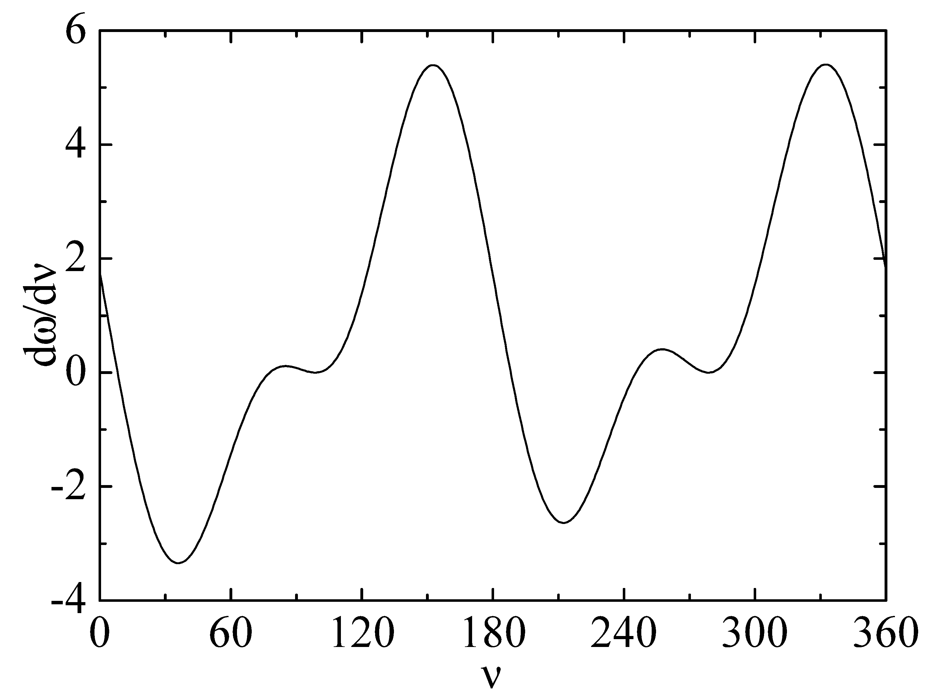
3.1. Precession of the Longitude of the Ascending Node

Some estimations on the unmodeled secular variation of the longitude of the ascending node have also been given by Fienga et al. [18]. This precession induced by the gravitomagnetic field is known as the Lense–Thirring effect in classical General Relativity [47]. In this section, we should calculate the extra precession induced by the field in Equation (3). Standard perturbation theory gives us the expression for the time derivative of the longitude of the ascending node (the angle between the radius vector at the point in which the orbit crosses the ecliptic point and the first point of Aries) as follows:

$${\displaystyle \frac{d\Omega }{dt}=\frac{r\mathcal{N}sin\nu }{Hsin\iota }=\sqrt{{\displaystyle \frac{p}{\mu }}}\mathcal{N}\frac{sin\nu }{sin\iota }\frac{1}{1+ϵcos(\nu -\omega )}}$$

(28)

where $\mathcal{N}$ is the normal component of the perturbation force as given in Equation (24). This expression can be integrated, as shown in the previous section, to obtain the advance of the longitude of the ascending node, Ω, for the planets. In doing so, we assume that the advance of the argument of the perihelion is $\Delta {\dot{\omega }}_{\text{S}}$_aturn = 0.15 milliarcsec per century, because this is the central value found with the INPOP10a model by Fienga et al. [18]. This implies that the coefficient β is $1/40$ the value listed in Table 2. Results for $\Delta \dot{\Omega }$ are listed in Table 3 and compared with the confidence intervals obtained with INPOP10a, although none of them is nonzero within the precision achieved. We notice that with the parameters $n=2$, $m=3$ and $n=4$, $m=5$, the predictions are consistent with the INPOP10a data within the error bars.

Table 2. Anomalous perihelion advance of the planets for the perturbation in Equation (3) and several pairs of the exponents n and m. The result is expressed in milliarcseconds per century. The values of β lie in the range $-0.019\le \beta \le 0.6824$. We have fitted the β parameter in order to obtain $\Delta {\dot{\omega }}_{\text{S}}$_aturn = −6 milliarcsec cy⁻¹ for a combination of parameters n, m. In the last case for $n=4$ and $m=5$, we used $\Delta {\dot{\omega }}_{\text{S}}$_aturn = 0.15 milliarcsec cy⁻¹ as the fitting condition. The result for the ephemerides analyzed by the model EPM2008 and two more recent studies are also shown.

(n,m)	$\Delta {\dot{\omega }}_{\text{M}}$ercury	$\Delta {\dot{\omega }}_{\text{V}}$enus	$\Delta {\dot{\omega }}_{\text{E}}$arth	$\Delta {\dot{\omega }}_{\text{M}}$ars	$\Delta {\dot{\omega }}_{\text{J}}$upiter	$\Delta {\dot{\omega }}_{\text{S}}$aturn	β
(1,0)	6.402	−57.82	−579.0	36.45	−18.0	−6.0	−0.00061
(2,0)	6.63	−61.44	−522.96	37.968	−19.2	−6.0	0.00065
(1,1)	50.97	−0.786	−156.96	−10.95	0.6	−6.0	−0.019
(2,1)	53.628	−0.87	−117.96	−11.676	0.66	−6.0	0.021
(3,1)	56.298	−0.966	−96.78	−12.	−0.678	−6.0	0.023
(2,3)	28.2	−0.012	−279.	−5.028	0.258	−6.0	0.116
(4,5)	3.216	−3.33 × 10−5	−56.46	−0.42	0.018	−6.0	0.6824
(4,5)	-0.0804	8.325 × 10−7	1.4115	0.0105	−0.00045	0.15	−0.017
EPM2008	−3.6 ± 5.0	−0.4 ± 0.5	−0.2 ± 0.4	0.1 ± 0.5	-	−6 ± 2	-
INPOP10a	0.4 ± 0.6	0.2 ± 1.5	−0.2 ± 0.9	−0.04 ± 0.15	−41 ± 42	0.15 ± 0.68	-
EPM2011	−2 ± 3	2.6 ± 1.6	0.19± 0.19	−0.02± 0.037	58.7 ± 28.3	−0.32 ± 0.47	-

Table 2. Anomalous perihelion advance of the planets for the perturbation in Equation (3) and several pairs of the exponents n and m. The result is expressed in milliarcseconds per century. The values of β lie in the range $-0.019\le \beta \le 0.6824$. We have fitted the β parameter in order to obtain $\Delta {\dot{\omega }}_{\text{S}}$_aturn = −6 milliarcsec cy⁻¹ for a combination of parameters n, m. In the last case for $n=4$ and $m=5$, we used $\Delta {\dot{\omega }}_{\text{S}}$_aturn = 0.15 milliarcsec cy⁻¹ as the fitting condition. The result for the ephemerides analyzed by the model EPM2008 and two more recent studies are also shown.

(n,m)	$\Delta {\dot{\omega }}_{\text{M}}$ercury	$\Delta {\dot{\omega }}_{\text{V}}$enus	$\Delta {\dot{\omega }}_{\text{E}}$arth	$\Delta {\dot{\omega }}_{\text{M}}$ars	$\Delta {\dot{\omega }}_{\text{J}}$upiter	$\Delta {\dot{\omega }}_{\text{S}}$aturn	β
(1,0)	6.402	−57.82	−579.0	36.45	−18.0	−6.0	−0.00061
(2,0)	6.63	−61.44	−522.96	37.968	−19.2	−6.0	0.00065
(1,1)	50.97	−0.786	−156.96	−10.95	0.6	−6.0	−0.019
(2,1)	53.628	−0.87	−117.96	−11.676	0.66	−6.0	0.021
(3,1)	56.298	−0.966	−96.78	−12.	−0.678	−6.0	0.023
(2,3)	28.2	−0.012	−279.	−5.028	0.258	−6.0	0.116
(4,5)	3.216	−3.33 × 10−5	−56.46	−0.42	0.018	−6.0	0.6824
(4,5)	-0.0804	8.325 × 10−7	1.4115	0.0105	−0.00045	0.15	−0.017
EPM2008	−3.6 ± 5.0	−0.4 ± 0.5	−0.2 ± 0.4	0.1 ± 0.5	-	−6 ± 2	-
INPOP10a	0.4 ± 0.6	0.2 ± 1.5	−0.2 ± 0.9	−0.04 ± 0.15	−41 ± 42	0.15 ± 0.68	-
EPM2011	−2 ± 3	2.6 ± 1.6	0.19± 0.19	−0.02± 0.037	58.7 ± 28.3	−0.32 ± 0.47	-

Table 3. The extra advance of the longitude of the ascending node for the planets as induced by the unconventional transversal gravitomagnetic field. The last column list the values and confidence intervals found by Fienga et al. [18] in milliarcseconds per century.

Parameters	$\Delta {\dot{\Omega }}_{\text{M}}$ercury	$\Delta {\dot{\Omega }}_{\text{V}}$enus	$\Delta {\dot{\Omega }}_{\text{E}}$arth	$\Delta {\dot{\Omega }}_{\text{M}}$ars	$\Delta {\dot{\Omega }}_{\text{J}}$upiter	$\Delta {\dot{\Omega }}_{\text{S}}$aturn
$n=1$, $m=0$	−0.970	−0.025	0.0038	−0.137	−0.0093	−0.0274
$n=2$, $m=0$	1.003	0.027	−0.0039	0.147	0.0083	0.0274
$n=1$, $m=1$	−0.811	0.000275	0.001375	0.2205	−0.034	0.0087
$n=2$, $m=1$	0.849	−0.0003	−0.0009	−0.228	0.0361	−0.0086
$n=3$, $m=1$	0.885	−0.0003	−0.0007	−0.236	0.0379	−0.0083
$n=2$, $m=3$	0.509	−7.1 × 10−6	−0.0024	−0.158	0.019	−0.0108
$n=4$, $m=5$	0.347	−1.8 × 10−7	−0.0026	−0.117	0.012	−0.0123
INPOP10a	1.4 ± 1.8	0.2± 1.5	0.0± 0.9	-0.05± 0.13	−41 ± 43	−0.1 ± 0.4

Table 3. The extra advance of the longitude of the ascending node for the planets as induced by the unconventional transversal gravitomagnetic field. The last column list the values and confidence intervals found by Fienga et al. [18] in milliarcseconds per century.

Parameters	$\Delta {\dot{\Omega }}_{\text{M}}$ercury	$\Delta {\dot{\Omega }}_{\text{V}}$enus	$\Delta {\dot{\Omega }}_{\text{E}}$arth	$\Delta {\dot{\Omega }}_{\text{M}}$ars	$\Delta {\dot{\Omega }}_{\text{J}}$upiter	$\Delta {\dot{\Omega }}_{\text{S}}$aturn
$n=1$, $m=0$	−0.970	−0.025	0.0038	−0.137	−0.0093	−0.0274
$n=2$, $m=0$	1.003	0.027	−0.0039	0.147	0.0083	0.0274
$n=1$, $m=1$	−0.811	0.000275	0.001375	0.2205	−0.034	0.0087
$n=2$, $m=1$	0.849	−0.0003	−0.0009	−0.228	0.0361	−0.0086
$n=3$, $m=1$	0.885	−0.0003	−0.0007	−0.236	0.0379	−0.0083
$n=2$, $m=3$	0.509	−7.1 × 10−6	−0.0024	−0.158	0.019	−0.0108
$n=4$, $m=5$	0.347	−1.8 × 10−7	−0.0026	−0.117	0.012	−0.0123
INPOP10a	1.4 ± 1.8	0.2± 1.5	0.0± 0.9	-0.05± 0.13	−41 ± 43	−0.1 ± 0.4

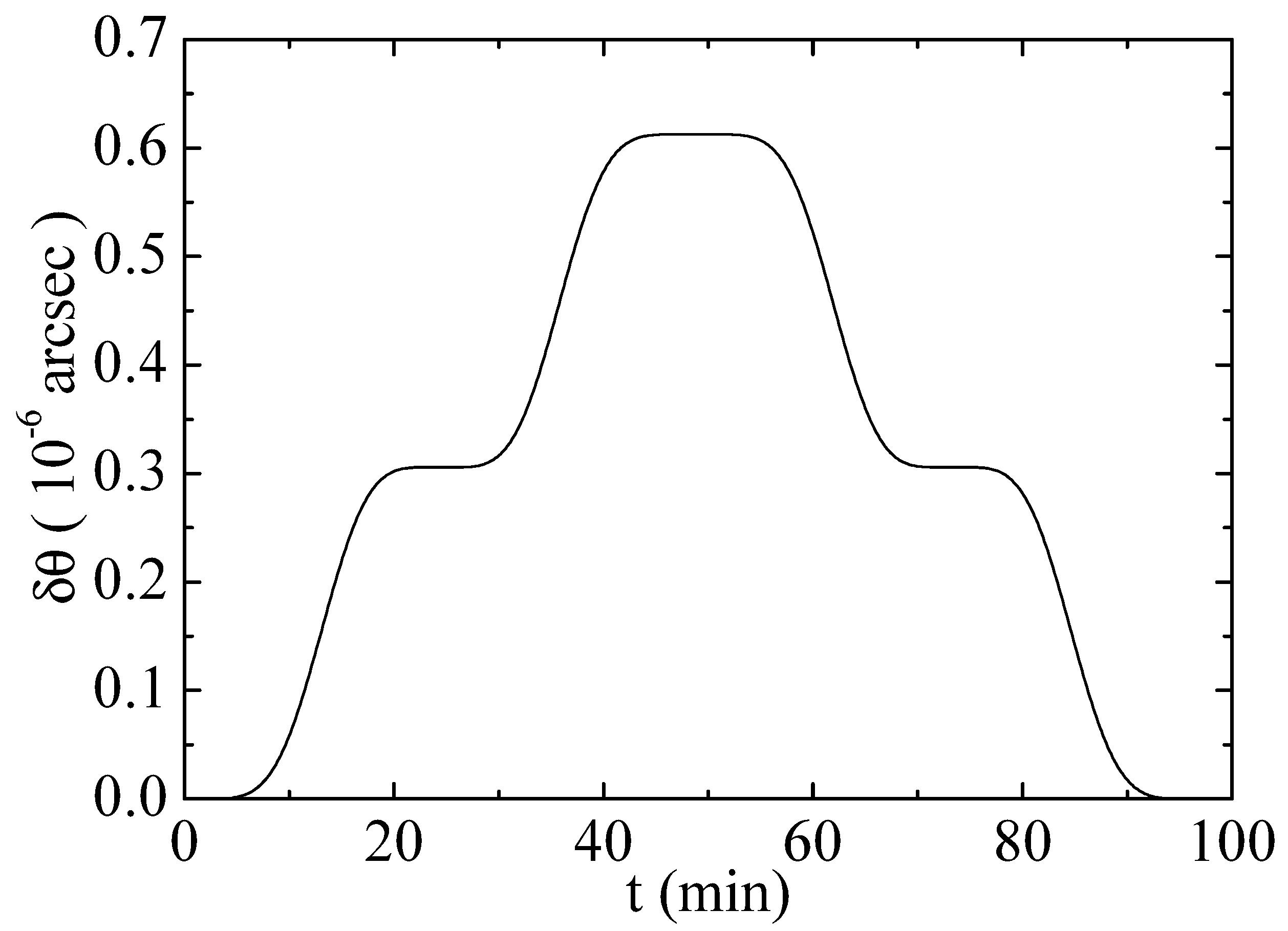
3.2. Contributions to the Gravity Probe B Experiment

It has been recently shown that a transversal gravitomagnetic component of the form given in Equation (1) with $n=1$, $m=1$ does not contribute secularly to the Gravity Probe B experiment (GPB) [39]. This recent experiment has confirmed the existence of the geodetic and the Lense–Thirring frame-dragging effect [48]. The first one is due to the movement of the satellite in the curved space-time around the Earth, while the second is associated with the gravitomagnetic field generated by the rotating Earth. Both of them produce small cumulative precessions on the onboard gyroscopes carefully mounted and monitored on the probe. For the low polar orbit of the GPB satellite (at a height $h=642$ km) these effects arise at right angles and could finally be separated [49].

The contribution from the proposed anomalous transversal field would be an oscillation in the north-south orientation of the gyroscopes to be obtained as the integral:

$$\begin{array}{ccc}\hfill \delta \theta \left(\nu \right)& =& {\displaystyle \beta W\frac{r_S}{R_E+h}{\int }_0^{\nu }{sin}^{n}x{cos}^{m}xdt}\hfill \\ & =& {\displaystyle \beta W\frac{r_S}{R_E+h}\frac{P}{2\pi }{(1-{ϵ}^2)}^{3/2}{\int }_0^{\nu }\frac{{sin}^{n}x{cos}^{m}x}{{(1+ϵcosx)}^2}dx}\hfill \end{array}$$

(29)

where $R_E=6378$ km is the average radius of the Earth, $h=642$ km is the altitude of the satellite, $ϵ=0.0014$ is the orbital eccentricity, $P=97.65$ min is the orbital period, and we have used Equation (26) to derive the result in terms of the true anomaly. In Figure 3, we have plotted the oscillation in the north-south orientation of the gyroscope induced by the transversal gravitomagnetic field for $n=4$, $m=5$ and $\beta =0.6824$. This value of β is the largest in Table 2, and it corresponds to the fitting of the EPM2008 data for the anomalous perihelion advance of Saturn. With this value of β, we find that the maximum deflection of the gyroscope in a single orbit is around $\delta \theta \simeq 6\times {10}^{-4}$ milliarcseconds and, consequently, totally negligible.

Figure 3. Evolution of the orientation angle of a gyroscope for the Gravity Probe B experiment under the influence of the gravitomagnetic field in Equation (3) for $n=4$, $m=5$ and $\beta =0.6824$. The angle, $\delta \theta$, is measured in units of a millionth of an arcsec and time, t, in minutes.

Figure 3. Evolution of the orientation angle of a gyroscope for the Gravity Probe B experiment under the influence of the gravitomagnetic field in Equation (3) for $n=4$, $m=5$ and $\beta =0.6824$. The angle, $\delta \theta$, is measured in units of a millionth of an arcsec and time, t, in minutes.

The Lense–Thirring effect has also been checked using the geodynamics satellites, LAGEOS and LAGEOS 2 [50]. Furthermore, the recently launched LARES should be used to refine the previous measurements. For a discussion about its ability to do so, see, e.g, Ciufolini et al. [51,52,53,54]. These spacecraft are completely covered by corner reflectors with the objective of becoming ideal targets for laser ranging. This configuration allows for a very precise monitoring of the satellite’s orbit. Ciufolini et al. have shown that from a combination of data obtained from the LAGEOS missions, a combined Lense–Thirring effect of $47.9$ milliarcseconds per year is deduced in good agreement with the prediction of General Relativity: $48.2$ milliarcseconds per year [51]. A debate on the level of accuracy reached is still ongoing [47,51,55,56,57]. As this is the most accurate determination of the Lense–Thirring effect to date, we should estimate the contribution of the putative transversal gravitomagnetic field proposed in this paper.

The orbits of the geodynamics satellites are almost circular. In the case of LAGEOS 1, the orbital eccentricity is $ϵ=0.0045$, with an inclination of $\iota =109.{84}^{\circ }$. LAGEOS 1 is located at a distance $a=5860$ km from the Earth’s center. We must also take into account that the Earth’s rotational axis is tilted $23.4^{\circ }$ with respect to the normal to the ecliptic plane. The longitude of the ascending node is precessing mainly as a consequence of the perturbations caused by the Earth’s geoid and the zonal harmonics. As we are interested in bounding the contribution of the extra gravitomagnetic field, we should chose the value of the longitude of the ascending node corresponding to the maximum effect. This corresponds to the maximum angle among the Earth’s rotational axis and the orbital inclination vector for the satellite’s orbit. Therefore, we take Ω_Earth = 0, ${\Omega }_{\text{LAGEOS}}=\pi$. The result for the instantaneous advance of the longitude of the ascending node in a single orbit is plotted in Figure 4, using $n=4$, $m=5$ and $\beta =0.6824$. We observe that the maximum effect is bounded by $0.15$ milliarcseconds per year, which lies outside the error bars for the present accuracy in the experimental result for the standard Lense–Thirring effect. Moreover, the net result of the extra gravitomagnetic Lense–Thirring effect, after one orbit, is null for circular orbits, as shown in Figure 4.

Figure 4. Instantaneous advance of the longitude of the ascending node for the LAGEOSsatellite in a single orbit, as determined from Equation (28), in milliarcseconds per year. Time, t, is measured in minutes. The parameters for the model are $n=4$, $m=5$ and $\beta =0.6824$.

Figure 4. Instantaneous advance of the longitude of the ascending node for the LAGEOSsatellite in a single orbit, as determined from Equation (28), in milliarcseconds per year. Time, t, is measured in minutes. The parameters for the model are $n=4$, $m=5$ and $\beta =0.6824$.

Therefore, we conclude that a transversal gravitomagnetic field sufficiently intense to impact on the Lense–Thirring precession of the planets, with contributions as those recently derived from the ephemerides models, is possible without conflicting with the results of the Gravity Probe B experiment and the determination of standard Lense–Thirring effect with the geodynamics satellites, LAGEOS and LARES.

4. Conclusions

The advance towards the verification of the General Theory of Relativity has been steady, but very slow in the century that has almost passed since its formulation [1]. Even today, we have no direct test proving the existence of gravitational waves. On the other hand, a final proof on the geodetic and gravitomagnetic effects of the rotating Earth has been recently achieved [48]. This is important for gravitational theory, because greater confidence will be obtained on the validity of General Relativity in contrast with many other alternatives. However, in this lengthy process, we cannot neglect the possible evenience of discovering of other minute effects and corrections not predicted by the original theory. These effects could open the door to a deeper understanding of the gravitational interaction. Examples of anomalies of this kind could already have been discovered, and it is possible that they will receive further confirmation in future studies. These are: (i) the anomalous increase of the astronomical unit [4,5]; (ii) the increase of the eccentricity of the orbit of the Moon unexplained by the tidal models of the DE421 ephemerides [3,10]; (iii) the extra precession of the longitude of the perihelion of some planets not predicted by classical perturbations, the standard Schwarzschild metric or the, even smaller, Lense–Thirring effect in General Relativity [15,58].

Assuming that these effects, if really existing, are not explainable conventionally, as observational errors or as the byproduct of flawed data analysis, we are confronted with a challenging problem in our understanding of gravitation. Some attempts have been made by invoking a cosmological origin, either empirically [4] or in terms of the behavior of the Solar System embedded in a cosmological background [10]. A slow variation of fundamental constants have also been proposed as a parsimonious explanation of both the astronomical unit anomaly and the anomalous increase of the eccentricity of the orbit of the Moon [6,59].

A third theoretical alternative is that the Lagrangian of General Relativity is incomplete, and there are more terms with small contributions to the Solar System dynamics than those dictated by the standard formulation of the theory [5]. Following this idea, we have proposed a transversal component of the gravitomagnetic field, and we have studied the resulting additional Lense–Thirring effect on the orbits of the planets for convenient values of the fitting parameter, β. Although the observed anomalies in the perihelion advance have very large error bars and differ from ephemerides to ephemerides, we have shown that an extra component of the gravitomagnetic field could fit them (at least for large values of the parameters n and m). On the other hand, the predictions for the perihelion advance of the Earth’s orbit are outside the error bars for most pairs n, m. Specially, we assume that the extra retrograde perihelion precession is the one found in the EPM2008 model. In this sense, the best agreement is found for the INPOP10a data. In this case, none of the observed anomalies is statistically significant.

Similarly, an extra unpredicted precession of the longitude of the ascending node could also be explained with the transversal gravitomagnetic component. Another interesting feature of this model is that it predicts both prograde and retrograde precessions depending upon the relative orientation of the Sun’s rotation axis and the planetary orbits. Evidence on unmodeled precessions of different signs have also been found [13,17,18,58].

Taking into account that the ephemerides models have still not achieved the desired accuracy, it is perhaps precipitate to speculate about the origin of such putative gravitomagnetic field. Surely, it will require an extension of the metric structure of space-time, but it cannot arise in standard Einstein–Cartan theory, because, in this theory, torsion does not propagate outside the bodies [40], but there are other alternatives to consider [41]. Further experimental, phenomenological and theoretical research is necessary to settle this issue in the future.

References

1. Will, C.M. The Confrontation between General Relativity and Experiment. Living Rev. Relativ. 2006, 9. [Google Scholar] [CrossRef]
2. Williams, J.G.; Turyshev, S.G.; Boggs, D.H. The past and present Earth-Moon system: The speed of light stays steady as tides evolve. Planet. Sci. 2014, 3. [Google Scholar] [CrossRef]
3. Iorio, L. On the anomalous secular increase of the eccentricity of the orbit of the moon. Mon. Not. R. Astron. Soc. 2011, 415, 1266–1275. [Google Scholar] [CrossRef]
4. Iorio, L. An empirical explanation of the anomalous increases in the astronomical unit and the lunar eccentricity. Astron. J. 2011, 142. [Google Scholar] [CrossRef]
5. Acedo, L. Anomalous post-Newtonian terms and the secular increase of the astronomical unit. Adv. Space Res. 2013, 52, 1297–1303. [Google Scholar] [CrossRef]
6. Acedo, L. A phenomenological variable speed of light theory and the secular increase of the astronomical unit. Phys. Essays 2013, 26, 567–573. [Google Scholar] [CrossRef]
7. Anderson, J.D.; Nieto, M.M. Astrometric solar-system anomalies. Proc. Int. Astron. Union 2010, 5, 189–197. [Google Scholar] [CrossRef]
8. Williams, J.G.; Boggs, D.H. Lunar Core and Mantle. What Does LLR See? In Proceedings of the 16th International Workshop on Laser Ranging, Poznan, Poland, 13–17 October 2008.
9. Williams, J.G.; Boggs, D.H.; Folkner, W.M. DE421 Lunar Orbit, Physical Librations, and Surface Coordinates. Available online: ftp://ssd.jpl.nasa.gov/pub/eph/planets/ioms/de421_moon_coord_iom.pdf (accessed on 18 May 2014).
10. Iorio, L. The Lingering Anomalous Secular Increase of the Eccentricity of the Orbit of the Moon: Further Attempts of Explanations of Cosmological Origin. Galaxies 2014, 2, 259–262. [Google Scholar] [CrossRef]
11. Pitjev, N.P.; Pitjeva, E.V. Constraints on dark matter in the solar system. Astron. Lett. 2013, 39, 141–149. [Google Scholar] [CrossRef]
12. Pitjeva, E.V. Updated IAA RAS planetary ephemerides EPM-2011 and their use in scientific research. Solar Syst. Res. 2013, 47, 386–402. [Google Scholar] [CrossRef]
13. Pitjeva, E.V.; Pitjev, N.P. Relativistic effects and dark matter in the Solar system from observations of planets and spacecraft. Mon. Not. R. Astron. Soc. 2013, 432, 3431–3437. [Google Scholar] [CrossRef]
14. Pitjeva, E.V.; Pitjev, N.P. Development of a planetary ephemerides EPM and their applications. Celest. Mech. Dyn. Astron. 2014, 119, 237–256. [Google Scholar] [CrossRef]
15. Iorio, L. The recently determined anomalous perihelion precession of Saturn. Astron. J. 2009, 137, 3615–3618. [Google Scholar] [CrossRef]
16. Iorio, L. The perihelion precession of Saturn, planet X/Nemesis and MOND. Open Astron. J. 2010, 3, 1–6. [Google Scholar] [CrossRef]
17. Pitjeva, E.V. Ephemerides EPM2008: The Updated Models, Constants, Data, Paper Presented at Journées “Systémes de Référence Spatio-temporels” and X Lohrmann-Kolloquium, Dresden, Germany, 2010. Available online: http://syrte.obspm.fr/jsr/journees2008/pdf/ (accessed on 23 September 2014).
18. Fienga, A.; Laskar, J.; Kuchynka, P.; Manche, H.; Desvignes, G.; Gastineau, M.; Cognard, I.; Theureau, G. The INPOP10a planetary ephemeris and its applications in fundamental physics. Celest. Mech. Dyn. Astron. 2011, 111, 363–385. [Google Scholar] [CrossRef] [Green Version]
19. Dvali, G.; Gabadadze, G.; Porrati, M. 4D Gravity on a Brane in 5D Minkowski Space. Phys. Lett. B 2000, 485, 208–214. [Google Scholar] [CrossRef]
20. Iorio, L. On the effects of Dvali Gabadadze Porrati braneworld gravity on the orbital motion of a test particle Class. Quantum Gravity 2005, 22, 5271–5281. [Google Scholar] [CrossRef]
21. Lue, A.; Starkman, G. Gravitational leakage into extra dimensions: Probing dark energy using local gravity. Phys. Rev. D 2003, 67. [Google Scholar] [CrossRef]
22. Khriplovich, I.B.; Pitjeva, E.V. Upper limits on density of dark matter in Solar System. Int. J. Mod. Phys. D 2006, 15, 615–618. [Google Scholar] [CrossRef]
23. Iorio, L. Solar system planetary orbital motions and dark matter J. Cosmol. Astropart. Phys. 2006, 2006. [Google Scholar] [CrossRef]
24. Sereno, M.; Jetzer, Ph. Dark matter versus modifications of the gravitational inverse-square law: Results from planetary motion in the Solar system. Mon. Not. R. Astron. Soc. 2006, 371, 626–632. [Google Scholar] [CrossRef]
25. Iorio, L. Solar System planetary tests of ċ/c. Gen. Relativ. Grav. 2010, 42, 199–208. [Google Scholar] [CrossRef]
26. Hees, A.; Folkner, W.M.; Jacobson, R.A.; Park, R.S. Constraints on modified Newtonian dynamics theories from radio tracking of the Cassini spacecraft. Phys. Rev. D. 2014, 89, 102002. [Google Scholar] [CrossRef]
27. Blanchet, L.; Novak, J. External field effect of modified Newtonian dynamics in the Solar System. Mon. Not. R. Astron. Soc. 2011, 412, 2530–2542. [Google Scholar] [CrossRef] [Green Version]
28. De la Fuente Marcos, C.; de la Fuente Marcos, R. Extreme trans-Neptunian objects and the Kozai mechanism: Signalling the presence of trans-Plutonian planets. Mon. Not. R. Astron. Soc. 2014, 443, L59–L63. [Google Scholar] [CrossRef]
29. Fernández, J.A. On the existence of a distant Solar companion and its possible effects on the Oort cloud and the observed comet population. Astroph. J. 2011, 726, 33. [Google Scholar] [CrossRef]
30. Trujillo, C.A.; Sheppard, S.S. A Sedna-like body with a perihelion of 80 astronomical units. Nature 2014, 507, 471–474. [Google Scholar] [CrossRef] [PubMed]
31. Iorio, L. Constraints on planet X/Nemesis from Solar System’s inner dynamics. Mon. Not. R. Astron. Soc. 2009, 400, 346–353. [Google Scholar] [CrossRef]
32. Iorio, L. Planet X revamped after the discovery of the Sedna-like object 2013 VP113. Mon. Not. R. Astron. Soc. Lett. 2014, 444, L78–L79. [Google Scholar] [CrossRef]
33. Iorio, L. Constraints on the location of a putative distant massive body in the Solar system planetary data. Celest. Mech. Dyn. Astron. 2012, 112, 117–130. [Google Scholar] [CrossRef]
34. Iorio, L. Perspectives of effectively constraining the location of a massive trans-Plutonian object with the New Horizons spacecraft: Trans-Plutonian object with the New Horizons spacecraft: A sensitivity analysis. Celest. Mech. Dyn. Astron. 2013, 116, 357–366. [Google Scholar] [CrossRef]
35. Lense, J.; Thirring, H. On the Influence of the Proper Rotation of Central Bodies on the Motions of Planets and Moons According to Einstein’s Theory of Gravitation. Phys. Z. 1918, 19, 156–163. [Google Scholar]
36. De Sitter, W. Einstein’s theory of gravitation and its astronomical consequences. Mon. Not. R. Astron. Soc. 1916, 76, 699–728. [Google Scholar] [CrossRef]
37. Iorio, L. Constraining the Angular Momentum of the Sun with Planetary Orbital Motions and General Relativity. Sol. Phys. 2012, 281, 815–826. [Google Scholar] [CrossRef]
38. Rindler, W. Relativity: Special, General, and Cosmological, 2nd ed.; Oxford University Press: Oxford, UK, 2006. [Google Scholar]
39. Acedo, L. The flyby anomaly: A case for strong gravitomagnetism? Adv. Space Res. 2014, 54, 788–796. [Google Scholar] [CrossRef]
40. Hehl, F.W.; von der Heyde, P.; David Kerlick, G.; Nester, J.M. General Relativity with Spin and Torsion: Foundations and Prospects. Rev. Mod. Phys. 1976, 48, 393–416. [Google Scholar] [CrossRef]
41. Hammond, R.T. Torsion Gravity. Rep. Prog. Phys. 2002, 65, 599–649. [Google Scholar] [CrossRef]
42. Giles, P. Time-Distance Measurements of Large-Scale Flows in the Solar Convection Zone. Ph.D. Thesis, Stanford University, Stanford, CA, USA, 1999. [Google Scholar]
43. Danby, J.M.A. Fundamentals of Celestial Mechanics, 2nd ed.; Willmann-Bell, Inc.: Richmond, VA, USA, 1988. [Google Scholar]
44. Pollard, H. Mathematical Introduction to Celestial Mechanics; Prentice-Hall Inc.: Englewood Cliffs, NJ, USA, 1966. [Google Scholar]
45. Arfken, G. Mathematical Methods for Physicists, 3rd ed.; Academic Press: Orlando, FL, USA, 1985. [Google Scholar]
46. NASA’s Planetary Factsheet. Available online: http://nssdc.gsfc.nasa.gov/planetary/factsheet/ (accessed on 23 September 2014).
47. Iorio, L.; Lichtenegger, H.I.M.; Ruggiero, M.L.; Corda, C. Phenomenology of the Lense-Thirring effect in the Solar System. Astrophys. Space Sci. 2011, 331, 351–395. [Google Scholar] [CrossRef]
48. Everitt, C.W.F.; DeBra, D.B.; Parkinson, B.W.; Turneaure, J.P.; Conklin, J.W.; Heifetz, M.I.; Keiser, G.M.; Silbergleit, A.S.; Holmes, T.; Kolodziejczak, J.; et al. Gravity Probe B: Final Results of a Space Experiment to Test General Relativity. Phys. Rev. Lett. 2011, 106, 221101. [Google Scholar] [CrossRef] [PubMed]
49. Everitt, C.W.F.; Adams, M.; Bencze, W.; Buchman, S.; Clarke, B.; Conklin, J.; DeBra, D.B.; Dolphin, M.; Heifetz, M.; Hipkins, D.; et al. Gravity Probe B Data Analysis: Status and Potential for Improved Accuracy of Scientific Results. Space Sci. Rev. 2009, 148, 53–69. [Google Scholar] [CrossRef]
50. Renzetti, G. History of the attempts to measure orbital frame-dragging with artificial satellites. Cent. Eur. J. Phys. 2013, 11, 531–544. [Google Scholar] [CrossRef]
51. Ciufolini, I.; Paolozzi, A.; Koenig, R.; Pavlis, E.C.; Ries, J.; Matzner, R.; Gurzadyan, V.; Penrose, R.; Sindoni, G.; Paris, C. Fundamental Physics and General Relativity with the LARES and LAGEOS satellites. Nucl. Phys. B (Proc. Suppl.) 2013, 243–244, 180–193. [Google Scholar] [CrossRef]
52. Ciufolini, I.; Paolozzi, A.; Pavlis, E.; Ries, J.; Gurzadyan, V.; Koenig, R.; Matzner, R.; Penrose, R.; Sindoni, G. Testing general relativity and gravitational physics using LARES satellite. Eur. Phys. J. Plus 2012, 127, 133:1–133:7. [Google Scholar] [CrossRef]
53. Renzetti, G. Are higher degree even zonals really harmful for the LARES/LAGEOS frame-dragging experiment? Can. J. Phys. 2012, 90, 883–888. [Google Scholar] [CrossRef]
54. Renzetti, G. First results from LARES: An analysis. N. Astron. 2013, 23, 63–66. [Google Scholar] [CrossRef]
55. Renzetti, G. Some reflections on the Lageos frame-dragging experiment in view of recent data analyzes. N. Astron. 2014, 29, 25–27. [Google Scholar] [CrossRef]
56. Iorio, L. An Assessment of the Systematic Uncertainty in Present and Future Tests of the Lense-Thirring Effect with Satellite Laser Ranging. Space Sci. Rev. 2009, 148, 363–381. [Google Scholar] [CrossRef]
57. Iorio, L.; Ruggiero, M.L.; Corda, C. Novel considerations about the error budget of the LAGEOS-based tests of frame-dragging with GRACE geopotential models. Acta Astronaut. 2013, 91, 141–148. [Google Scholar] [CrossRef]
58. Iorio, L. Preliminary bounds of the gravitational local position invariance from Solar system planetary precessions. Mon. Not. R. Astron. Soc. 2014, 437, 3482–3489. [Google Scholar] [CrossRef]
59. Bel, L. Earth and Moon orbital anomalies. 2014. [Google Scholar]