
On the Number of Galaxies at High Redshift


Dipartimento di Fisica, Università degli Studi di Torino, via P.Giuria 1, Turin I-10125, Italy
Galaxies 2015, 3(3), 129-155; https://doi.org/10.3390/galaxies3030129
Submission received: 6 March 2015
/
Revised: 27 August 2015
/
Accepted: 28 August 2015
/
Published: 3 September 2015
Abstract
:The number of galaxies at a given flux as a function of the redshift, z, is derived when the z-distance relation is non-standard. In order to compare different models, the same formalism is also applied to the standard cosmology. The observed luminosity function for galaxies of the zCOSMOS catalog at different redshifts is modeled by a new luminosity function for galaxies, which is derived by the truncated beta probability density function. Three astronomical tests, which are the photometric maximum as a function of the redshift for a fixed flux, the mean value of the redshift for a fixed flux, and the luminosity function for galaxies as a function of the redshift, compare the theoretical values of the standard and non-standard model with the observed value. The tests are performed on the FORS Deep Field (FDF) catalog up to redshift and on the zCOSMOS catalog extending beyond . These three tests show minimal differences between the standard and the non-standard models.
Keywords:
cosmology; observational cosmology; distances, redshifts, radial velocities, spatial distribution of galaxies; magnitudes and colors, luminositiesPACS classifications:
98.80.-k; 98.80.Es; 98.62.Py; 98.62.Qz1. Introduction
The linear correlation between the expansion velocity, v, and , the distance in Mpc, is
where is the Hubble constant , with when h is not specified, c is the velocity of light, see Mohr et al. [1], and z is the redshift defined as
with and denoting respectively the wavelengths of the observed and emitted lines as determined from the lab source, the so called Doppler effect. This linear relation can be derived from first principles, namely general relativity (GR), and is only a low-z limit of a more general relation in standard cosmology. The presence of a velocity in the previous equation has pointed the standard cosmology towards an expanding universe. The previous equation also contains a linear relation between distance and redshift, and this has pointed the experts in plasma physics towards an explanation of the redshift in terms of the interaction of light with the electrons of the intergalactic medium (IGM). In terms of plasma physics, the expansion velocity of the universe becomes a pseudo-velocity because the Universe is supposed to be Euclidean and static. The conjecture here adopted is now outlined: the redshift should be considered as a spectroscopic measure independent of the adopted cosmology. An example of this conjecture can be found at the home page of the Supernova Cosmology Project (SCP) “All the analyses were developed with cosmology hidden.” The main physical explanations for the redshift are: a Doppler shift, which means an expanding universe, a general relativistic effect, see [2], a plasma effect, see [3], and a tired light effect as suggested by [4,5]. More details on the various theories which explain the cosmological redshift can be found in [6]. A point of discussion: The presence of physical effects which explain the redshift allows us to speak of a Euclidean universe in which the distances are evaluated with the Pythagorean theorem. In a Euclidean universe, the main parameters are , z, and the distance, d, but the velocity of expansion is virtual rather than real. The aim of having a Euclidean universe is the explanation of the astronomical variables such as the redshift and the absolute magnitude and count of galaxies without GR.
Concerning the value of and , we will adopt recent values as obtained by a mixed model which uses the cosmic microwave background (CMB) measurements at high redshift and the baryon acoustic oscillation (BAO), see [7],
Hubble’s constant is explained in the dynamical relativistic models beginning with [8,9]. Recently, research in the framework of modern theories on an accelerating universe has been focussed on measuring cosmological parameters such as and , see [10,11]. In the last years, the enormous progress in astronomical observations has increased the available data for galaxies up to z = 3.36, see the FORS Deep Field (FDF) catalog, which is made up of 300 galaxies with known spectroscopic redshift, see [12,13]. Another high redshift catalog is zCOSMOS, which is made up of 9697 galaxies up to z = 4, see [14]. These data demand a new formalism for the number of galaxies as a function of the redshift. At the same time, Hubble’s law can be inserted into a more precise physical framework. In order to cover these questions, Section 2 reviews some old and new derivations of Hubble’s law as well the magnitude system, and Section 3 derives a new relation for the number of galaxies as a function of the redshift. Section 5 introduces a relativistic model for the number of galaxies as a function of the redshift and Section 6 deals with the luminosity function for galaxies at different redshifts.
2. Basic Formulae
The change of frequency of light in a gravitational framework [15], a photo-absorption process between the photon and the electron in the intergalactic medium, see Equation (3) in [4], or a plasma effect, see Equation (50) in [3], all give
We can isolate the distance in Equation (1), obtaining the linear relation
In standard cosmology, one cannot use the previous approximation when inserting d into Equation (10) for redshifts larger than ≈ 0.1. The previous equation needs to be generalised in standard cosmology when with the use of both the “Hubble function”, see Equation (58), and the luminosity distance, see Equation (62). The expression for the distance, d, in the nonlinear Equation (5) gives the relation
Figure 1.
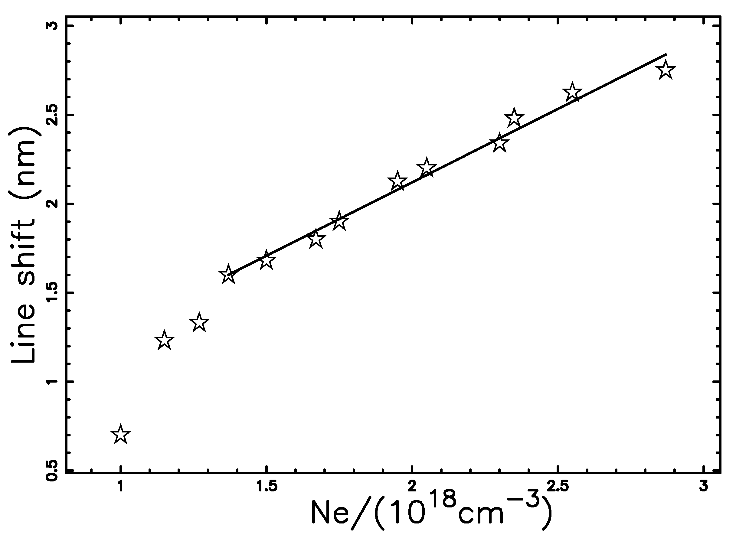
HgI 435.83 nm line shifts versus the electron density, data as extracted by the author from Figure 7 in [16] (empty stars) and linear regime (full line).
Figure 1.
HgI 435.83 nm line shifts versus the electron density, data as extracted by the author from Figure 7 in [16] (empty stars) and linear regime (full line).

A Taylor expansion around of this equation gives
In the limit , the linear distance, , and the nonlinear, d, are equal. The laboratory results of the line shift in dense and hot plasmas can be found in [17,18,19,20,21]. As a first example, the experimental verification of the redshift of the spectral line of mercury as due to the surrounding electrons can be found in Figure 1, see also [22]. A second example is given by the Balmer series line emitted by laser-produced hydrogen. A linear fit of the data in Table 1 in [23] gives the relation for the redshift of the line
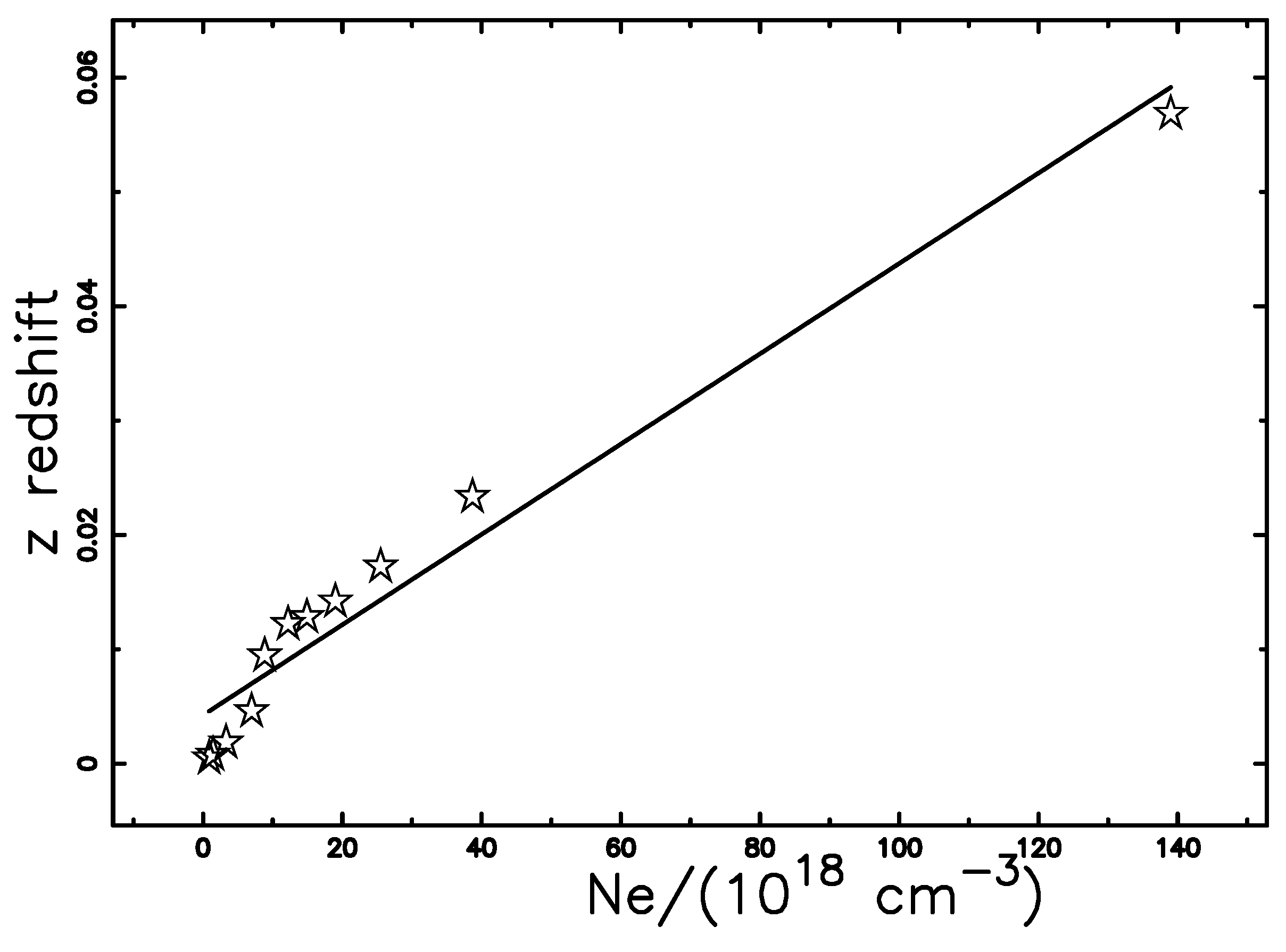
where is the electron number density. This linear relation can be visualized in Figure 2. The previous relation shows a laboratory redshift as a function of a growing density. In astrophysical plasma, we are interested in the redshift as a function of the distance when the temperature of the medium is 3 K, as known from the cosmic microwave background (CMB), and its mean density is extremely low.
Figure 2.
Redshift of the line versus the electron density, data as extracted by the author from Table 1 in [23] (empty stars) and linear fit (full line).
Figure 2.
Redshift of the line versus the electron density, data as extracted by the author from Table 1 in [23] (empty stars) and linear fit (full line).

Therefore the previous laboratory experiment is illustrative rather than quantitative.
2.1. Magnitude System
The absolute magnitude of a galaxy, M, is connected with the apparent magnitude m through the relation
The nonlinear absolute magnitude as a function of the redshift as given by the nonlinear Equation (7) is
The previous formula predicts, from a theoretical point of view, an upper limit on the maximum absolute magnitude which can be observed in a catalog of galaxies characterized by a given limiting magnitude. The previous curve can be connected with the Malmquist bias, see [24,25], which was originally applied to the stars and later on to the galaxies by [26]. We now define the Malmquist bias as the systematic distortion in luminosity or absolute magnitude for the effective range of galaxies due to a failure in detecting those galaxies with fainter luminosity or high absolute magnitude at large distances.
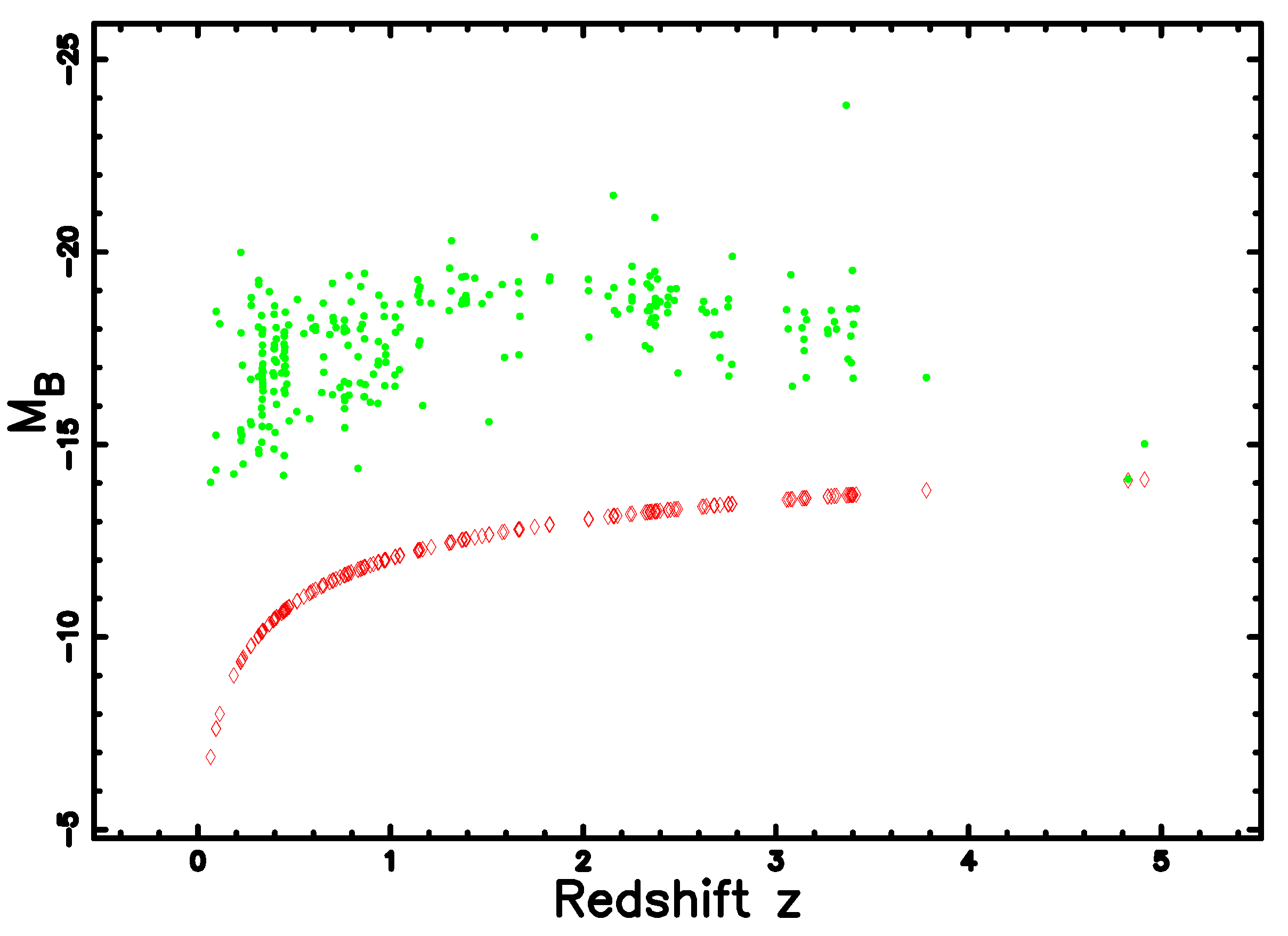
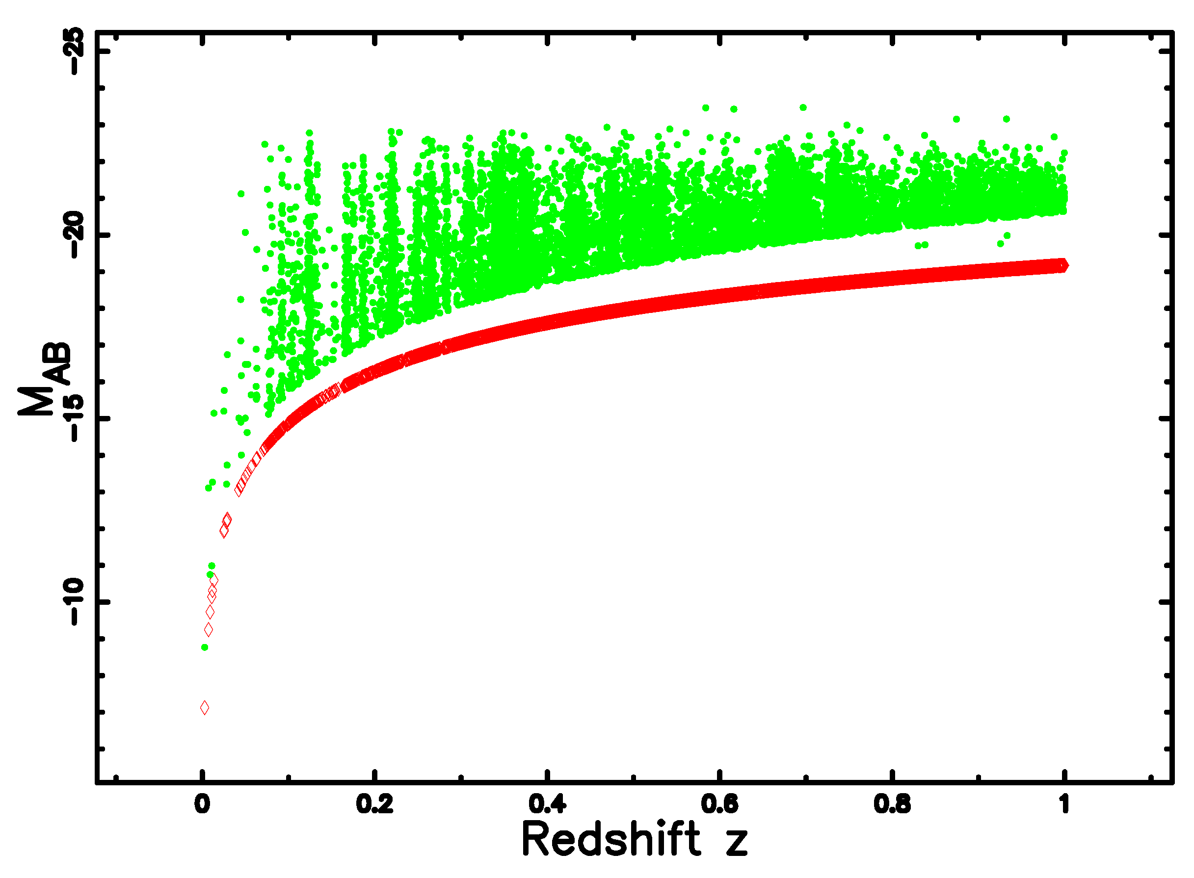
Figure 3 shows such a curve, the Malmquist bias, for the FDF catalog. The well measured spectroscopic redshift, the blue and red apparent magnitude of the FDF data, can be found at the Strasbourg Astronomical Data Centre (CDS). Figure 4 shows the curve of the Malmquist bias for the zCOSMOS catalog. A careful examination of Figure 3 and Figure 4 allows to conclude that all the galaxies are in the region over the border line of the Malmquist bias and the number of observed galaxies decreases with increasing z as theoretically predicted.
Figure 3.
The blue absolute magnitude computed with the nonlinear Equation (11) for 263 galaxies belonging to the FORS Deep Field (FDF) catalog versus the well measured redshift. The lower theoretical curve as represented by the nonlinear Equation (11) is the red thick line when = 30.33, which is the maximum apparent magnitude of the catalog, = 5.48 and (green points). The redshift covers the range .

In a Euclidean, non-relativistic, and homogeneous universe, the flux of radiation without attenuation, f, expressed in units of , where represents the luminosity of the sun, is
where d represents the nonlinear distance of the galaxy expressed in Mpc, see Equation (7). The relation connecting the absolute magnitude, M, of a galaxy to its luminosity is
where is the reference magnitude of the sun in the considered bandpass.
The flux expressed in units of as a function of the apparent magnitude is
and the inverse relation is
Once a band is fixed, we have a reference magnitude of the sun in that band. We give a few examples: band in SDSS = 6.38, band B in FDF = 5.48 and band B in zCOSMOS = 4.08.
Figure 4.
The B absolute magnitude M computed with the nonlinear Equation (11) for 9697 galaxies belonging to the zCOSMOS catalog versus the redshift. The lower theoretical curve as represented by the nonlinear Equation (11) is the red thick line when = 23.2, = 4.08 and (green points). The redshift covers the range .

2.2. Tired Light
Assume that the photon loses energy, E, in a way proportional to its energy:
The coefficient is assumed to be proportional to the averaged number density of the IGM, n,
and therefore
We now replace the energy where h is Planck’s constant,
and we convert the frequency to the wavelength,
The speed of light, c, is assumed to be constant,
where is the original wavelength. On introducing the redshift
We obtain
where is the averaged number density. The Hubble constant can be introduced with the following meaning,
obtaining
The distance d has the same dependence on the photo-absorption/plasma process as given by Equation (7)
The observed flux without the absorption of our galaxy is
and the distance modulus for tired light is
A generalization of the concept of tired light can be obtained by inserting a supplementary absorption of the light, i.e., Compton scattering, see formula (51) in [3]:
where β is a variable parameter which is 1 when only tired light is considered and 3 when the Compton scattering is added. Here we have invoked the Compton scattering as a possible source of absorption but the parameter β can be considered a regulating parameter of an unknown scattering mechanism. The distance modulus of generalized tired light without galactic extinction is
Hubble’s constant can be extracted from this equation as a function of the distance modulus ():
and, as a practical example, when = 43.834 and , which is the case with SN C-001 in the Union 2.1 compilation, we have when β = 2.032, which is the same value quoted in our Introduction.
A first comparison can be done with the distance modulus in a plasma environment as given by Equation (7) in [27] without galactic extinction:
see Equation (7) in [27]. A second comparison can be done with the historical equation (23) in [28], which is the relation for the steady-model
We briefly recall that Sandage [28] used two explosive models, a Friedman model [8,9] and a steady state model [29].
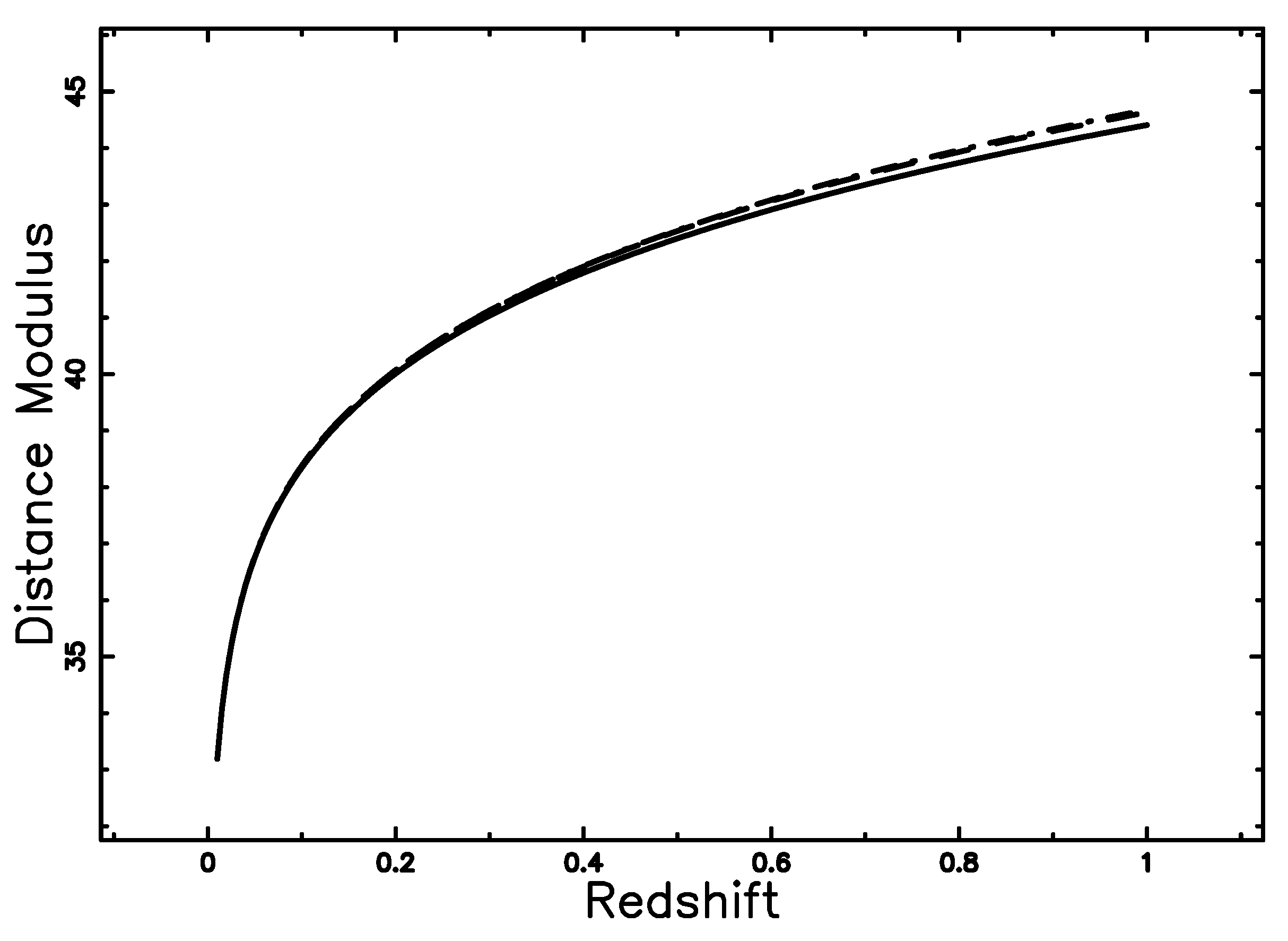
Figure 5 presents the behavior of the three distance moduli here considered as functions of the redshift. We now outline how formula (26) dates back to the year 1929. The original formula for the change of frequency of light in a gravitational framework is due to [15]:
Figure 5.
Distance modulus for the generalized tired light as given by Equation (30) (full line) with β = 2.7, for a plasma as given by Equation (32) (dashed line), and for the steady-model as given by Equation (33) (dot-dash-dot-dash line).

Here, ν is the frequency, G is the Newtonian gravitational constant, ρ is the density in g/cm, D is the distance after which the perturbing effect begins to fade out, L is the distance, and c is the speed of light. We make the change of variables , , , and , which means
On repeating the previous procedure, we obtain formula (26).
There is actually a debate on the existence of tired light in laboratory experiments. Here we use tired light as a simple theory to model a more complex interaction between light and the intergalactic plasma.
2.3. The Luminosity Function
The Schechter function, introduced by Schechter [30], provides a useful fit for the luminosity function (LF) for galaxies:
Here, α sets the slope for low values of L, is the characteristic luminosity, and is a normalization. The equivalent distribution in absolute magnitude is
where is the characteristic magnitude as derived from the data. The scaling with h is and .
3. N–z Relation
This section evaluates the number of galaxies as a function of the redshift, firstly assuming a linear relation and secondly a nonlinear relation between redshift and distance. The evaluations are done on a sphere of radius r which is identified with the chosen distance. The main statistical test is the :
where n is the number of bins, is the theoretical value, is the experimental value represented in terms of frequencies, and is the error computed as the square root of .
3.1. The Linear Case
The joint distribution in z and f for galaxies, see formula (5.133) in [31] or formula (1.104) in [32] or formula (1.117) in [33], is
where , and represent the differential of the solid angle, the redshift, and the flux, respectively, and Φ is the Schechter LF. The critical value of z, , is
The number of galaxies in z and f as given by formula (39) has a maximum at , where
which can be re-expressed as
or introducing the two observable variables, and ,
These two formulas, which model the photometric maximum, are not reported in chapter 5 of [31].
3.2. The Nonlinear Case
We assume that and
where r is the distance; in our case, d is as represented by the nonlinear Equation (7). The relation between and is
The joint distribution in z and f for the number of galaxies is
where δ is the Dirac delta function.
The evaluations of the integral over luminosity and distances gives
The number of galaxies in z and f as given by formula (48) has a maximum at , where
or introducing the two observable variables, and
The total number of galaxies comprised between a minimum value of flux, , and a maximum value of flux , for the Schechter LF can be computed through the integral
This integral does not have an analytical expression and we must perform a numerical integration.
The above integral does not have an analytical expression, and should be numerically evaluated. The differences between the formulas of this subsection and the formulas in Chapter 5 of [31] are that our formalism is built to cover high values of the redshift, against the low values of the redshift of the standard approach. Both models are built in the framework of a Euclidean universe.
4. Astrophysical Applications
We processed two catalogs in order to test the theoretical formulae: the FDF and the zCOSMOS. These two catalogs differ for the number of galaxies and parameters of the Schechter luminosity function (LF) for galaxies. We now review the three parameters of the Schechter LF: α is fixed, is not relevant because we equalize the theoretical maximum in frequencies, and is allowed to vary in order to match the observed frequencies. The observed mean redshift of galaxies with a flux f or m, , is evaluated by the following algorithm.
- (1)
- A window in apparent magnitude or flux is chosen around m or f.
- (2)
- All the galaxies which fall in the window are selected.
- (3)
- The mean value in redshift of N selected galaxies is and the uncertainty in the mean, , is where s is the standard deviation, see formula (4.14) in [34].
4.1. The FDF Catalog
The pencil beam catalog FDF has a solid angle of ≈ 5.6 sq arcmin, or around the south galactic pole, and covers the interval in redshift. In particular, we selected the 263 galaxies with spectroscopical redshift and we processed the B band which has the range in apparent magnitude mag. The reference magnitude for FDF in the B band is = 5.48. The Schechter LF for galaxies has been widely used to parametrise the LF in FDF as a function of the redshift. As an example in band B, in the range with , see Figure 5 in [12]. We have maintained but we make variable and specify it in the captions of the figures. The distribution of the spectroscopic redshifts in the FDF is presented in Figure 6 and a comparison should be made with the distribution of photometric redshifts, see Figure 2 in [13].
Figure 7 presents the number of observed galaxies in the FDF catalog at a random apparent magnitude and Figure 8 reports the theoretical number of galaxies as function of redshift and apparent magnitude. Here we adopted the law of the rare events or Poisson distribution in which the variance is equal to the mean, i.e., the error bar is given by the square root of the frequency. An enlarged discussion on the validity of this approximation can be found in [35].
Figure 6.
The galaxies of the FDF catalog are organized in frequencies versus spectroscopic redshift. The redshift covers the range and the histogram’s interval is 0.1.
Figure 6.
The galaxies of the FDF catalog are organized in frequencies versus spectroscopic redshift. The redshift covers the range and the histogram’s interval is 0.1.

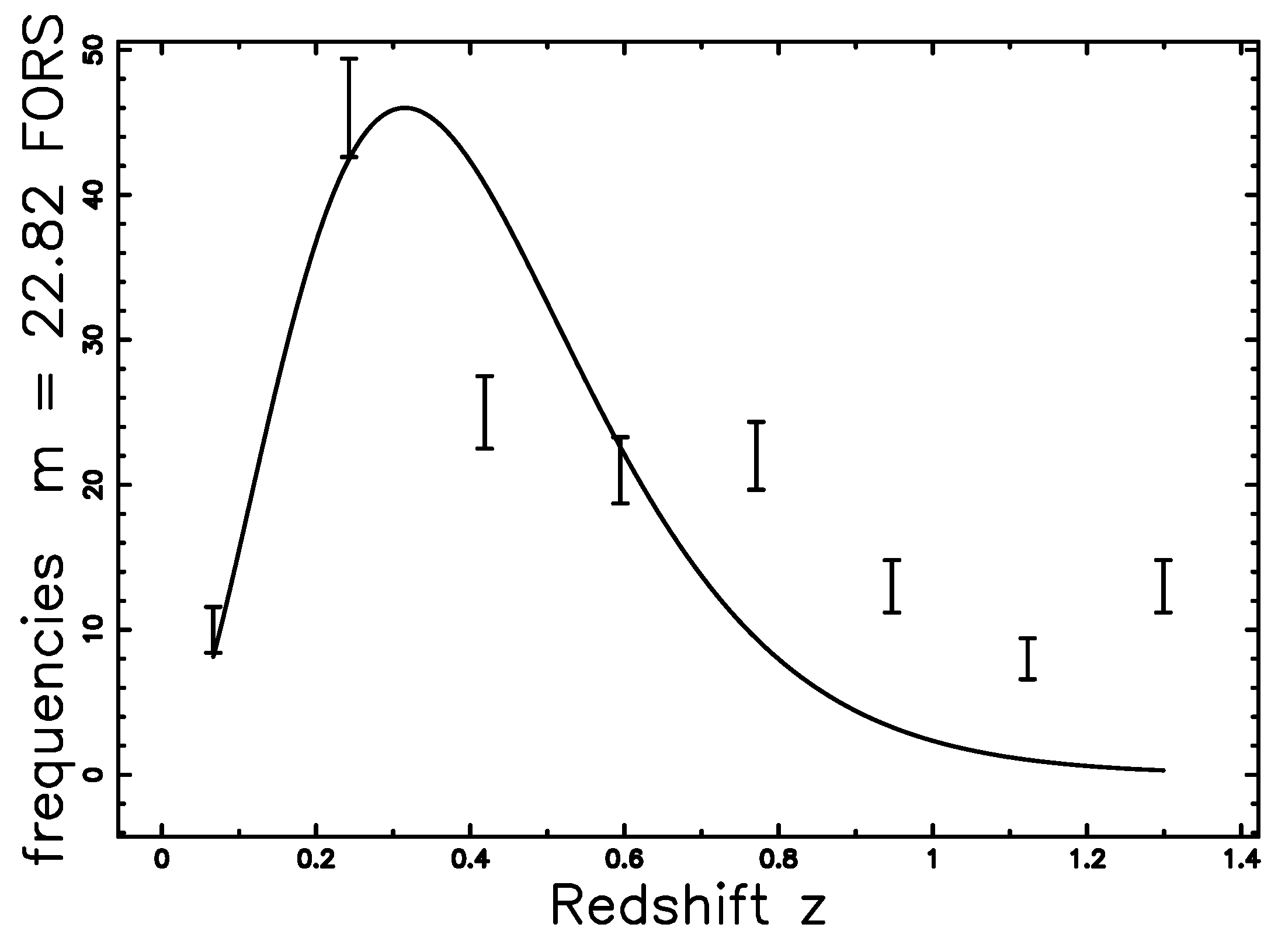
Figure 7.
The galaxies of the FDF catalog with or are organized in frequencies versus spectroscopic redshift. The redshift covers the range and the histogram’s interval is 0.18. The maximum frequency of observed galaxies is at , 77.8, and the number of bins is 8. The full line is the theoretical curve generated by as given by the application of the Schechter luminosity function (LF) which is Equation (48) with , and .

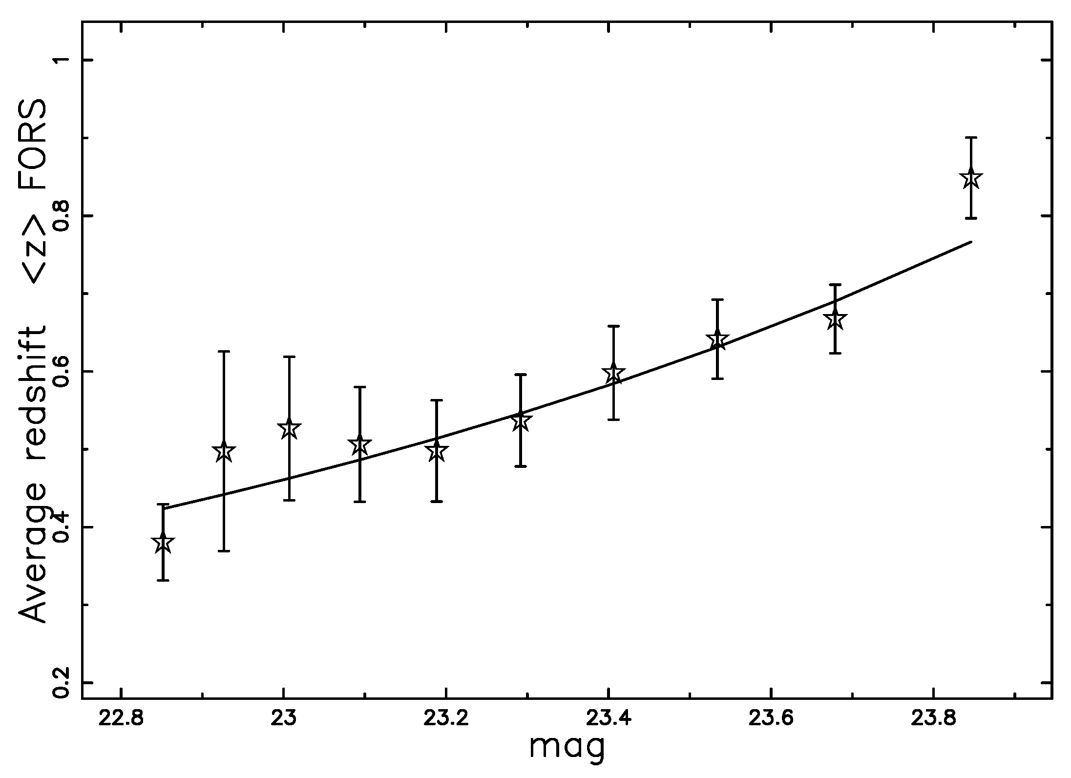
A careful examination of Figure 3 in [13] gives the maximum frequency of galaxies with well measured spectroscopic redshift in the FDF at . The mean redshift of galaxies as a function of the apparent magnitude for the FDF catalog is presented in Figure 9, which shows an acceptable agreement between the data (empty stars) and the theoretical values (full line).
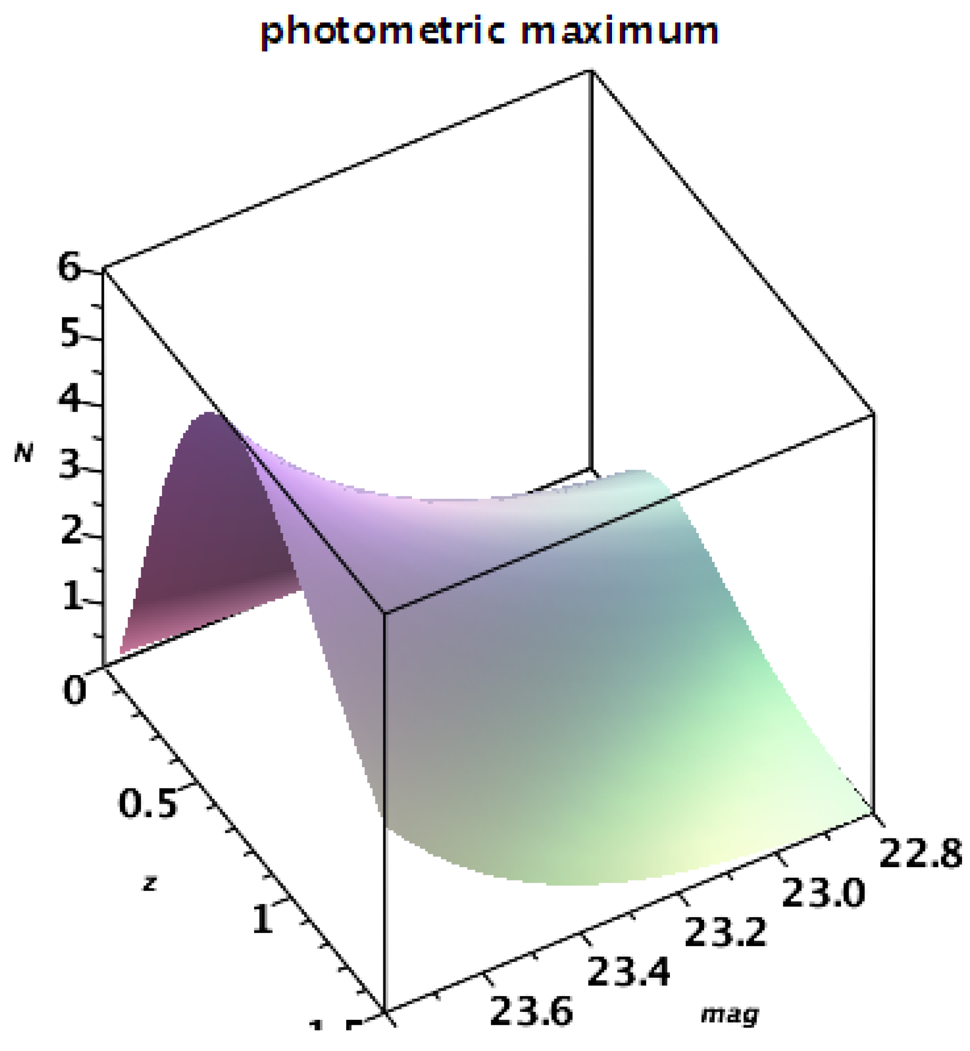
Figure 8.
The theoretical number of galaxies of the FDF catalog as afunction of redshift and apparent magnitude represented as a 3D surface, parameters as in Figure 7.
Figure 8.
The theoretical number of galaxies of the FDF catalog as afunction of redshift and apparent magnitude represented as a 3D surface, parameters as in Figure 7.


4.2. The zCOSMOS Catalog
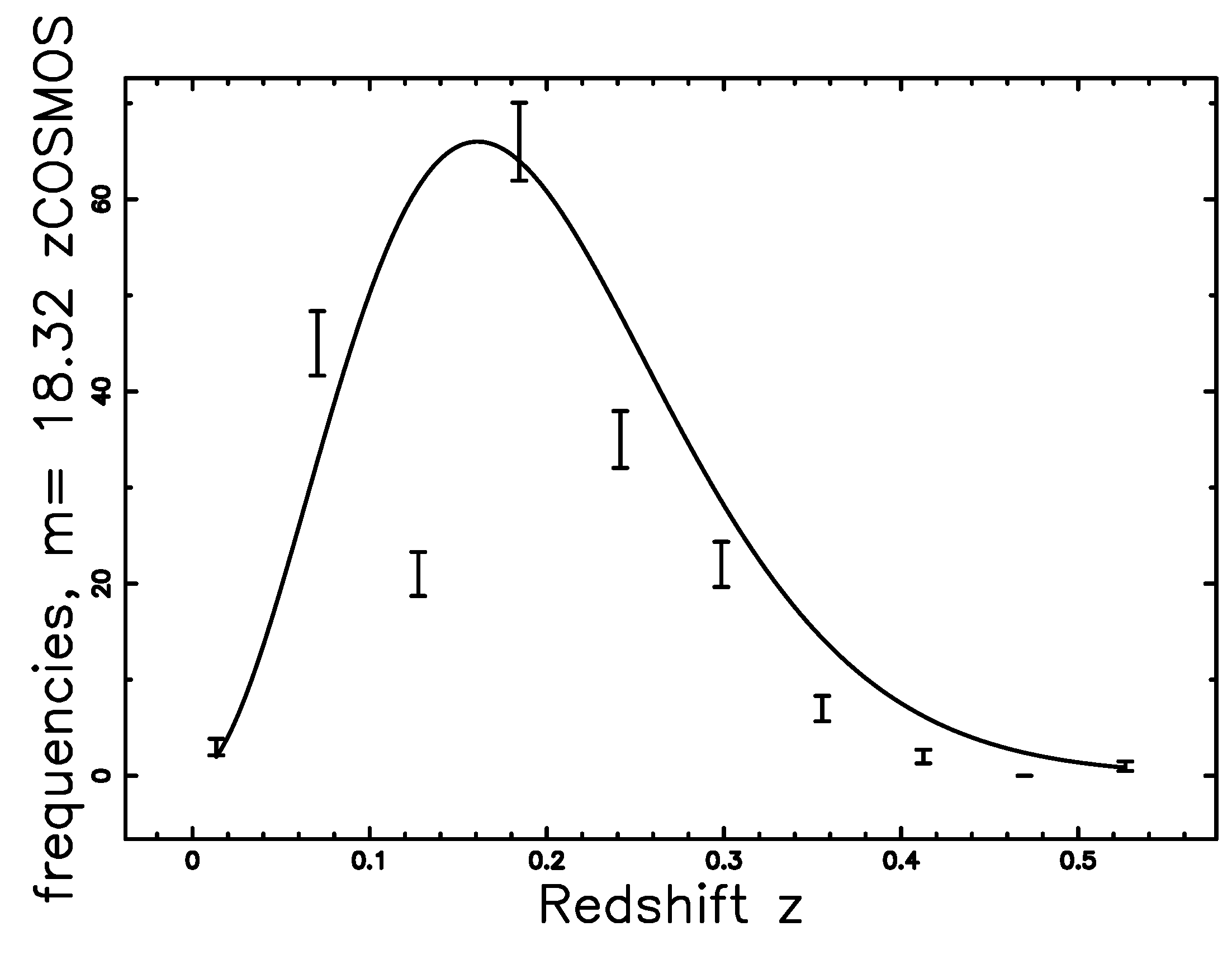
The zCOSMOS bright redshift 10k catalog, which covers a solid angle or sr, consists of 9697 galaxies in the the interval in redshift and range in the band mag, see [14]. The reference magnitude for zCOSMOS in the band is = 4.08, see Table 2.1 in [36]. The number of galaxies as a function of the redshift does not have a continuous behavior: rather, we are in the presence of an alternating behavior of voids and relative maxima, see Figure 10. This nonhomogeneous spatial distribution of galaxies can be made continuous by introducing bigger intervals in the computation of the frequencies, e.g., a histogram interval equal to 0.1. Figure 11 presents the number of observed galaxies in the zCOSMOS catalog for a given apparent magnitude.
Figure 10.
The galaxies of the zCOSMOS catalog are organized in frequencies versus spectroscopic redshift. The redshift covers the range and the histogram’s interval is 0.02.
Figure 10.
The galaxies of the zCOSMOS catalog are organized in frequencies versus spectroscopic redshift. The redshift covers the range and the histogram’s interval is 0.02.

Figure 11.
The galaxies of the zCOSMOS catalog with or are organized in frequencies versus spectroscopic redshift. The redshift covers the range and the interval in the histogram is 0.1. The error bar is given by the square root of the frequency (Poisson distribution) . The maximum frequency of observed galaxies is at , 147.3, and the number of bins is 10. The full line is the theoretical curve generated by as given by the application of the Schechter LF, which is Equation (48) with , and .

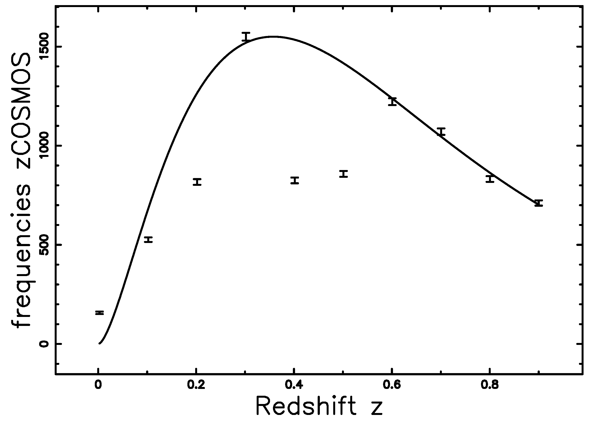
The total number of galaxies, , can be computed with the integral represented by Equation (51), see Figure 12.
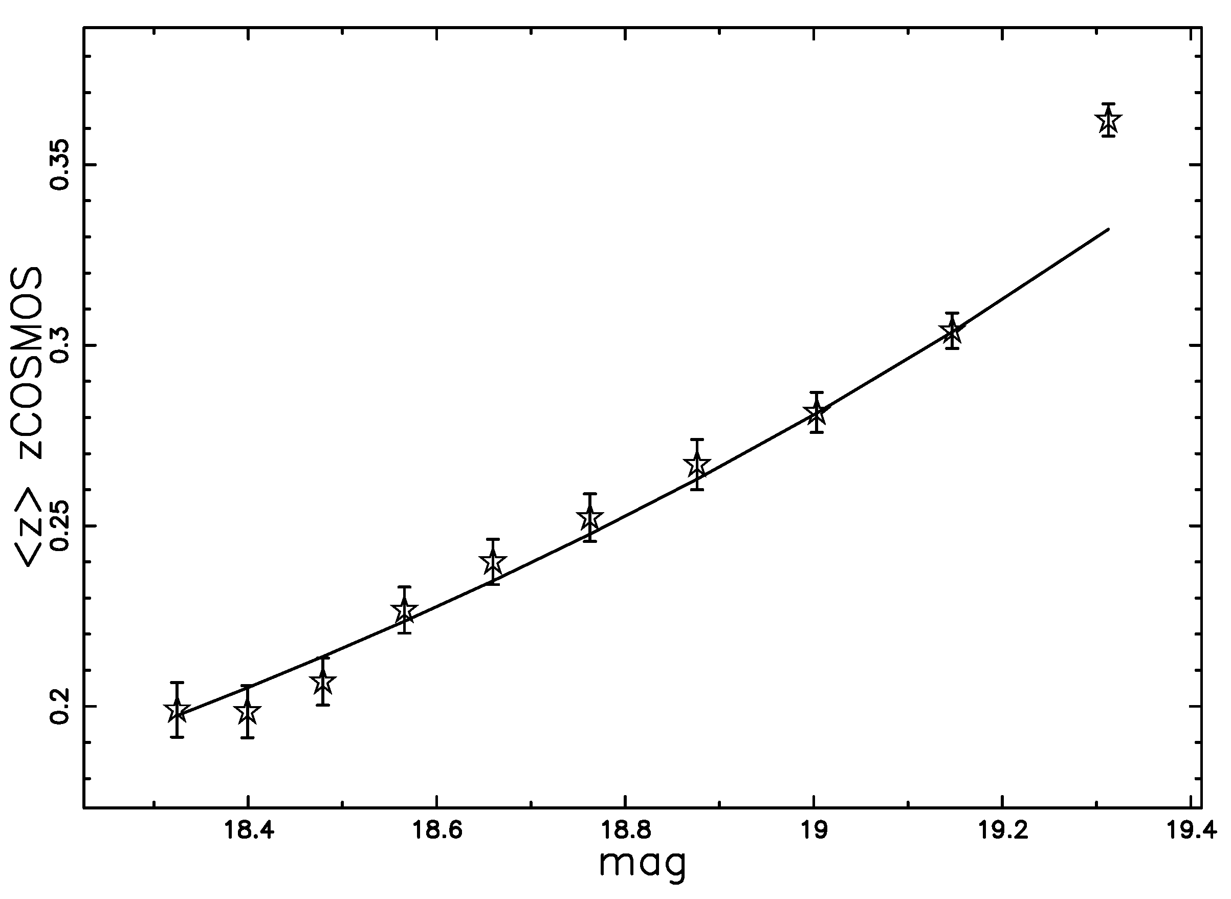
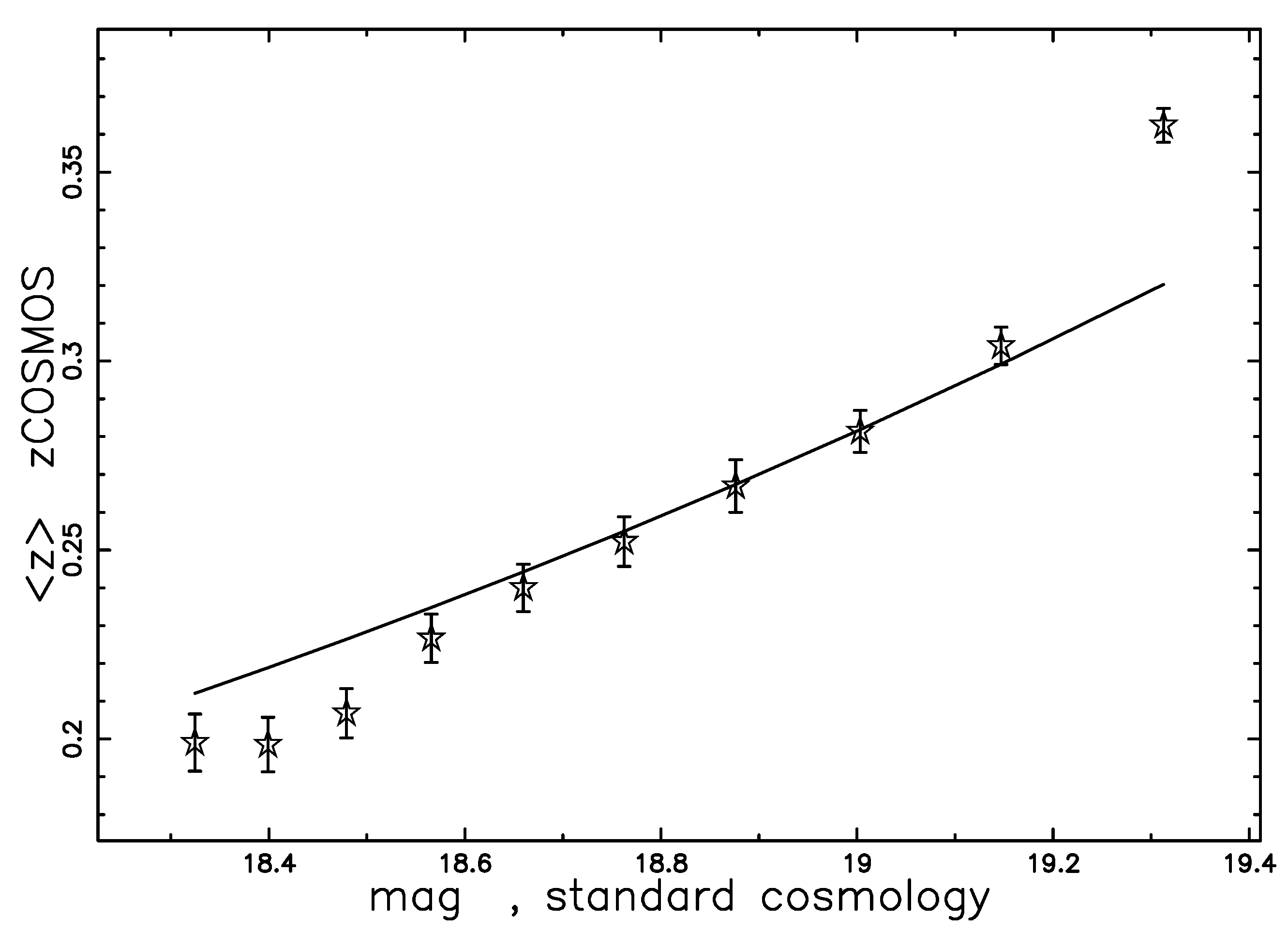
The mean redshift of galaxies as a function of the apparent magnitude for zCOSMOS is presented in Figure 13.
Figure 12.
All the galaxies of the zCOSMOS catalog, organized in frequencies versus spectroscopic redshift. The redshift covers the range and the interval in the histogram is 0.1. The error bar is given by the square root of the frequency (Poisson distribution) . The maximum frequency of all observed galaxies is at , 1864.65, and the number of bins is 10. The full line is the theoretical curve generated by as given by the numerical integration of Equation (51) with , and .


5. The Relativistic Case
The possibility of deriving an analytical result for the number of galaxies as a function of the redshift in the relativistic case is connected with the availability of an analytical expression for the luminosity distance. We now use the same symbols as in [37] and we define the Hubble distance as
We then introduce a first parameter
where G is the Newtonian gravitational constant and is the mass density at the present time. A second parameter is
where λ is the cosmological constant, see [31]. The two previous parameters are connected with the curvature by
The comoving distance, , is
where is the “Hubble function”
The transverse comoving distance is
An analytic expression for can be obtained when :
A new form for when is
The luminosity distance is
which in the case of becomes
and the distance modulus
We now return to : the ration between the differential of the luminosity distance and the differential of the redshift is
This means that we have an analytical expression for the differential when . This analytical differential will be inserted later on in Equation (67). The inverse relation between distance and redshift, now denoted by , is
The joint distribution in z and f for the number of galaxies in the relativistic case is
and its explicit value is
where
and
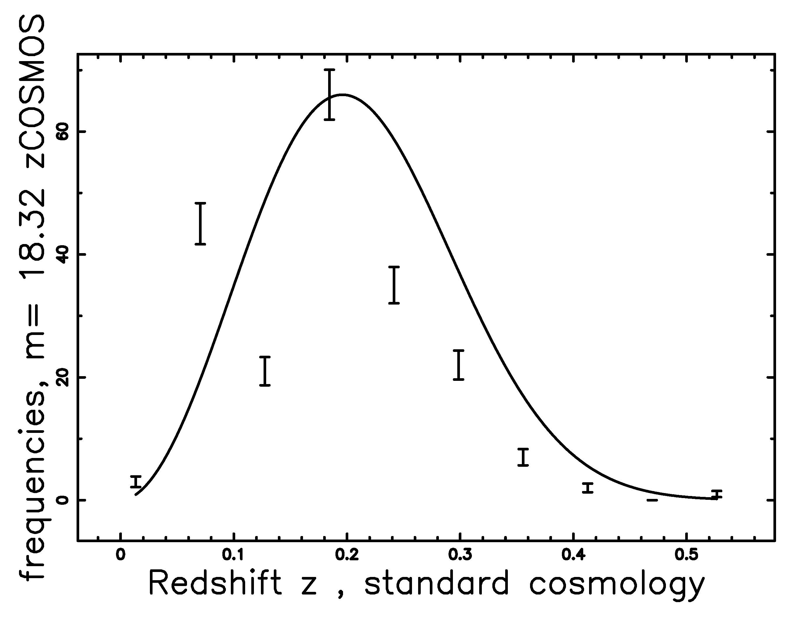
Figure 14 presents the number of observed galaxies in the zCOSMOS catalog for a given apparent magnitude in the relativistic case; we adopted the value of because it is the concordance value, see [7].
The mean numerical redshift of galaxies as a function of the apparent magnitude for zCOSMOS is presented in Figure 15 for the relativistic case.
The observed galaxy number over-density on cosmological scales up to second order in perturbation theory with all relativistic effects that arise by observing on the past lightcone are discussed in [38,39].
Figure 14.
The galaxies of the zCOSMOS catalog with the same parameters of Figure 11 are organized in frequencies versus spectroscopic redshift. The full line is the theoretical curve generated by as given by the application of the Schechter LF in the relativistic case, which is Equation (68) with , , and ; =95.68 when the number of bin is 10.

Figure 15.
Average observed redshift, , as function of the apparent magnitude for the zCOSMOS catalog (empty stars) and theoretical full line, , as given by a numerical integration. Theoretical parameters as in Figure 14.
Figure 15.
Average observed redshift, , as function of the apparent magnitude for the zCOSMOS catalog (empty stars) and theoretical full line, , as given by a numerical integration. Theoretical parameters as in Figure 14.

6. Evolutionary Effects
The main problem in modeling the LF as a function of the redshift is that the low luminosity galaxies progessively disappear. This observational fact can be solved by adopting a truncated probability density function (PDF). The beta distribution is defined in and the beta with scale PDF is defined in . On introducing a truncation in the beta PDF at low values, we can model the observed LF as a function of the redshift, see formula (34) in [40]. Once the random variable X is substituted with the luminosity L, we obtain a new LF for galaxies, Ψ,
where is a normalization factor which defines the overall density of galaxies, a number per cubic Mpc. The constant is
and , are the lower, upper values in luminosity and is the regularized hypergeometric function [41,42]. The averaged luminosity, , is
where
The relations connecting the absolute magnitude M, and of a galaxy to the respective luminosities are
where is the absolute magnitude of the sun in the considered band. The beta truncated LF in magnitude is
where
This LF contains the five parameters α, β, , , which can be derived from the operation of fitting the observational data and which characterize the considered band, see [43]. The number of variables can be reduced to three once and are identified with the maximum and the minimum absolute magnitude of the considered sample. A further reduction of parameters can be realized in the case of a well defined catalog of galaxies, e.g., zCOSMOS, where = −23.47 mag, , and = 4.08. The low luminosity bound (high magnitude) can be modeled in the classic case by extracting the absolute magnitude from Equation (28) which represents the distance modulus for tired light by
where is the limiting apparent magnitude, which for zCOSMOS is mag. With the above choice of parameters, the observed LF for zCOSMOS as a function of the redshift has only one free parameter, , which can be easily derived from the fit of the histograms. The observed LF for zCOSMOS can be built by adopting the following algorithm.
- (1)
- A value for the redshift is fixed, z, as well as the thickness of the layer, .
- (2)
- All the galaxies comprised between z and are selected.
- (3)
- The absolute magnitude can be computed from Equation (28) which represents the distance modulus for tired light.
- (4)
- The distribution in magnitude is organized in frequencies versus absolute magnitude.
- (5)
- The frequencies are divided by the volume, which is , where r is the considered radius, is the thickness of the radius, and Ω is the solid angle of ZCOSMOS.
- (6)
- The error in the observed LF is obtained as the square root of the frequencies divided by the volume.
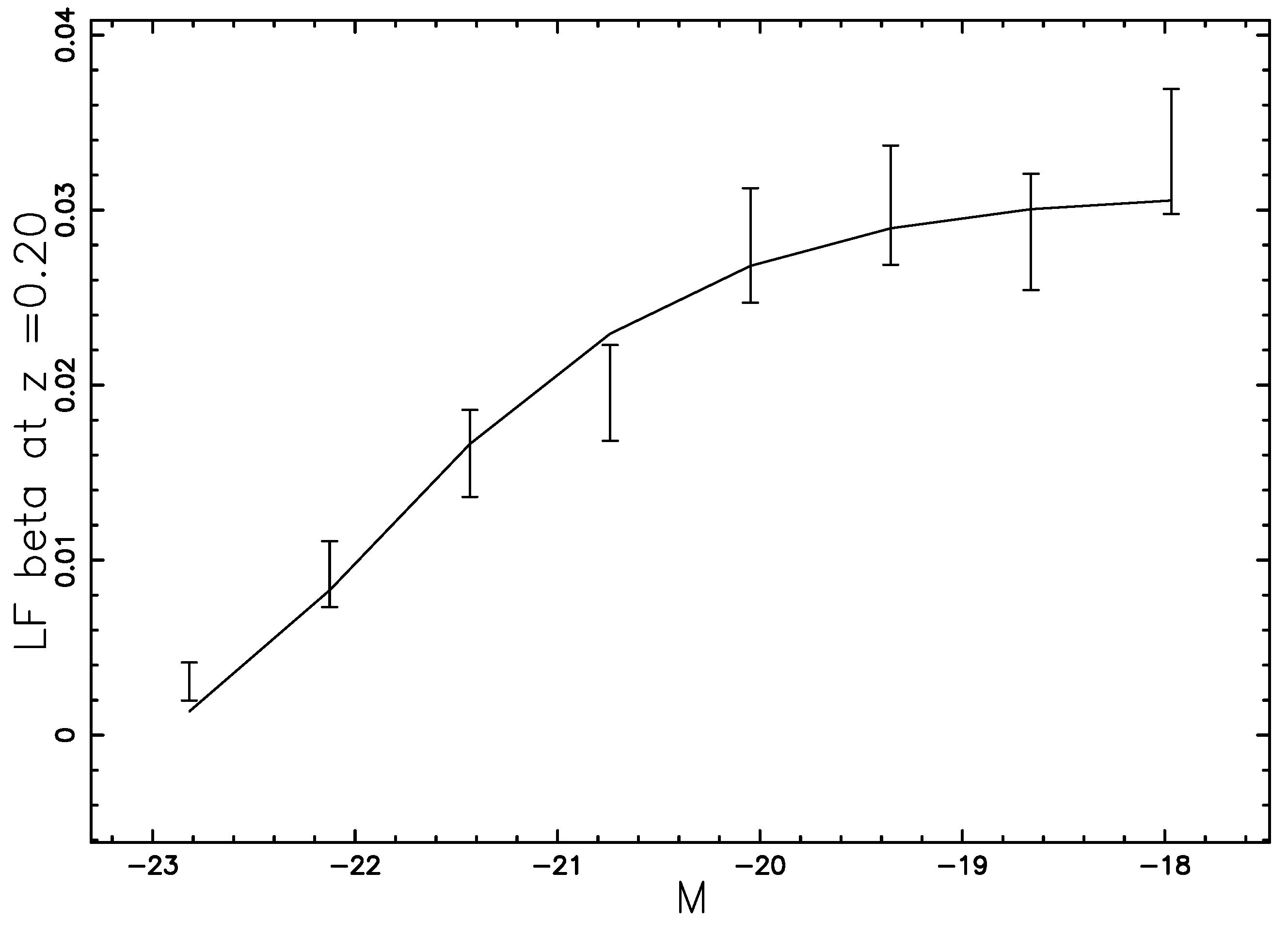
Figure 16, Figure 17 and Figure 18 present the LF of zCOOSMOS as well the fit with the truncated beta LF at z = 0.7, respectively.
In the relativistic case, we can extract the absolute magnitude from Equation (64), which represents the distance modulus when :
Figure 16.
The luminosity function data of zCOSMOS are represented with error bars. The continuous line fit represents our beta LF (77), the parameters are , = 0.05 and NDIV = 8, which means .
Figure 16.
The luminosity function data of zCOSMOS are represented with error bars. The continuous line fit represents our beta LF (77), the parameters are , = 0.05 and NDIV = 8, which means .

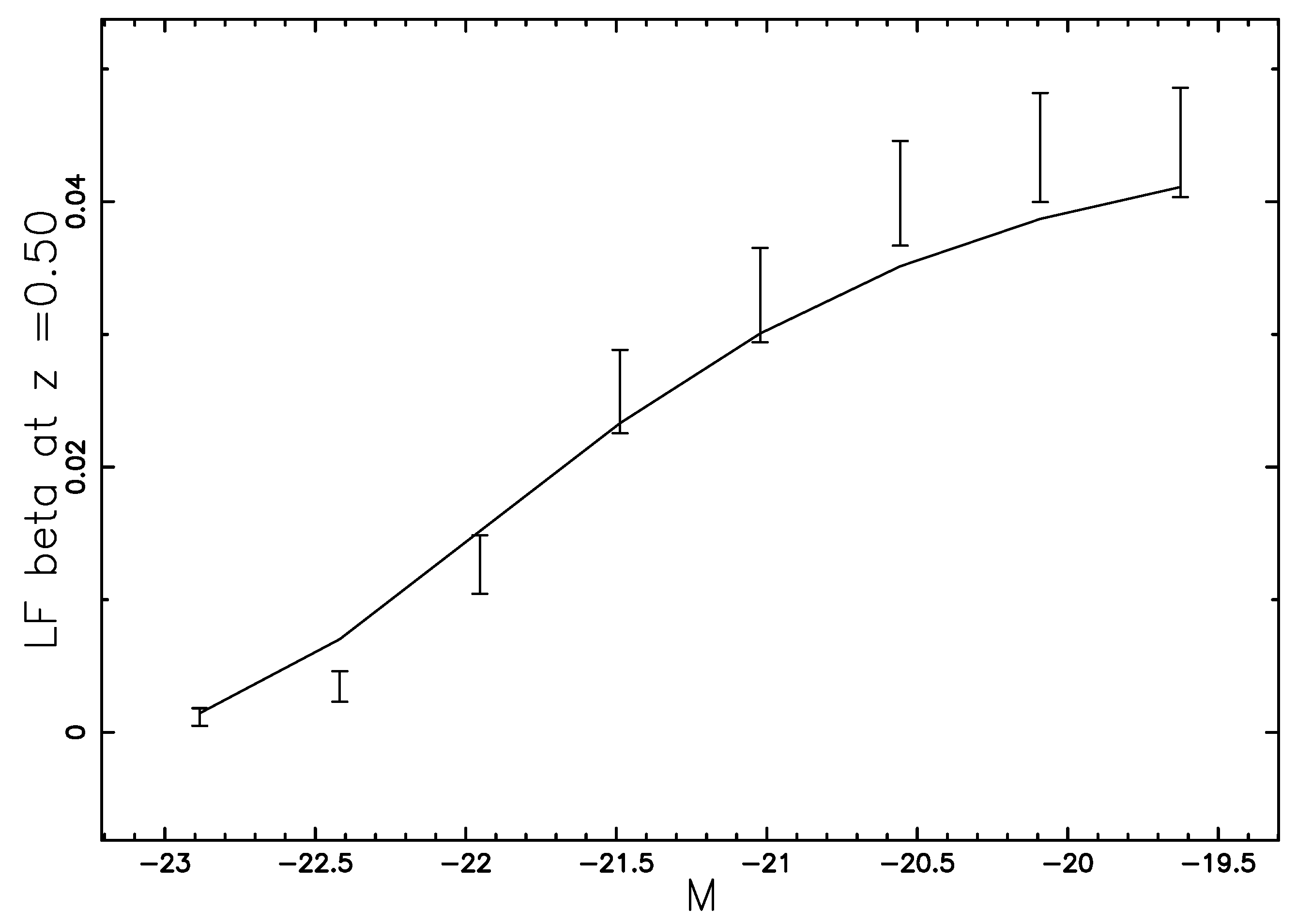
Figure 17.
The luminosity function data of zCOSMOS are represented with error bars. The continuous line fit represents our beta LF (77), the parameters are , = 0.05, and NDIV = 8, which means = 16.71.
Figure 17.
The luminosity function data of zCOSMOS are represented with error bars. The continuous line fit represents our beta LF (77), the parameters are , = 0.05, and NDIV = 8, which means = 16.71.

Figure 18.
The luminosity function data of zCOSMOS are represented with error bars. The continuous line fit represents our beta LF (77), the parameters are , = 0.03, and NDIV = 4, which means = 8.76.
Figure 18.
The luminosity function data of zCOSMOS are represented with error bars. The continuous line fit represents our beta LF (77), the parameters are , = 0.03, and NDIV = 4, which means = 8.76.

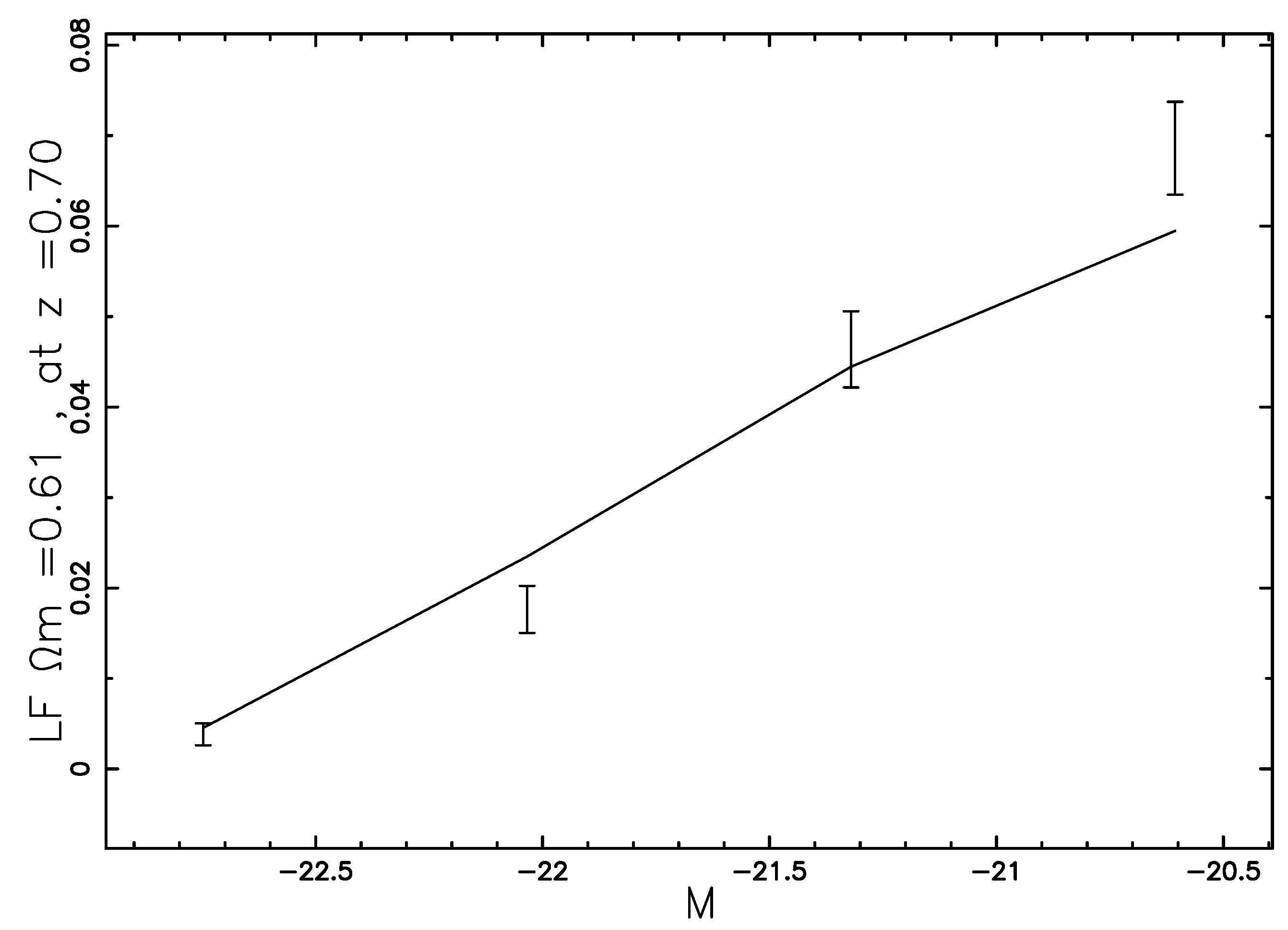
Figure 19 presents the LF of zCOOSMOS as well as the fit with the truncated beta LF when in the relativistic case.
Figure 19.
The luminosity function data of zCOSMOS are represented with error bars. The continuous line fit represents our beta LF (77) in the relativistic case. The input parameters are , , , = 0.03 and NDIV = 4, which means = 8.78.
Figure 19.
The luminosity function data of zCOSMOS are represented with error bars. The continuous line fit represents our beta LF (77) in the relativistic case. The input parameters are , , , = 0.03 and NDIV = 4, which means = 8.78.

7. Conclusions
7.1. Results
A nonlinear formulation of Hubble’s law allows determinaing an old/new relation for the distance as a function of the redshift, see Equation (7). This distance, when inserted in the definition of the joint distribution in z and f for the number of galaxies, allows the determination of a new relation, see Equation (48). Two photometric tests were done for 263 galaxies belonging to the FDF catalog and for 9697 galaxies belonging to the zCOSMOS catalog. The first test is dedicated to the photometric maximum in redshift, for which it is possible to derive an analytical expression as a function of the flux, see Equation (49), or the apparent magnitude, see Equation (49); this results in Figure 7 and Figure 11.
A second test is dedicated to the average redshift, for which a numerical integration of Equation (52) should be done; it results in Figure 9 and Figure 13.
The same formalism can also be applied to the relativistic case once the relativistic luminosity distance is given, see Equation (63). In the standard cosmology or relativistic case the the joint distribution in z and f for the number of galaxies is given by Equation (68). A comparison between the Euclidean and relativistic model can be made on the photometric maximum as represented by Figure 11 and Figure 14. The test gives for the Euclidean case, as represented by Equation (47) and for the relativistic case as represented by Equation (68), but large oscillations are present in the observed frequencies and therefore the definitive answer is remanded to future efforts.
The observed LF for galaxies can be modeled by a truncated beta LF, see Equation (77). This new LF with an appropriate choice of parameters has only one free parameter, which is the number of galaxies per cubic Mpc, , and this parameter decreases with the redshift. The high magnitude bound, , can be modeled both by a Euclidean model as given by Equation (79) and by a relativistic model, , as given by Equation (80). As an example, the third test for the observed LF for galaxies at gives = 8.76 for the Euclidean case and = 8.78 for the relativistic case when and .
7.2. Generalizated Tired Light
The presence of the factor β for adjustable tired light, see Equations (29) and (30), poses the problem of its determination. Equation (30), which represents the distance modulus, can be calibrated on the database of supernova (SN) of type Ia. A careful determination of β and can provide a better determination of the Malmquist bias, as represented by Figure 3 and Figure 4, which present a lack of galaxies just above the red lines.
7.3. Tired Light versus GR
The new distance modulus as represented by Equation (30) requires a careful comparison with the standard LCDM. In the case of LCDM with , an analytical solution for the luminosity distance exists and allows the determination of the relation between the differential of the distance and the differential of the redshift, see Equation (65).
In the case of , an analytical expression for the luminosity distance does not exist, and as a consequence we do not have at the moment of writing a relation between the differential of the distance and the differential of the redshift. The use of the Padé approximant can produce analytical results for the luminosity distance, see [44,45]; this approximation will be the subject of future research.
7.4. The Cells
The cellular structure of our universe, see as an example Figure 10, is now the greatest inconvenience to the application of the continuous models for the number of galaxies as a function of the redshift, and perhaps an explanation for why the theoretical lines do not fit the data, as an example see Figure 12. We briefly recall that there is an actual debate on the dimension of the universe which is modeled by , where N is the number of galaxies, R the radius of the considered sphere, and D the dimension. An homogeneous universe means . In the concordance model, D makes a transition to at scales between 40 and 100 Mpc, see [46]. An accurate analysis of 2MASS Photometric Redshift catalogue (2MPZ), shows an agreement with the standard cosmological model; the homogeneous regime is reached faster than a class of fractal models with D < 2.75, see [47]. As an example of non-homogeneity the value has been reported in [48] where the 2MASS Redshift Survey catalog was analysed.
Acknowledgments
I am grateful to the anonymous referee for useful suggestions which have changed the structure of the paper.
Conflicts of Interest
The author declare no conflict of interest.
References
- Mohr, P.J.; Taylor, B.N.; Newell, D.B. CODATA recommended values of the fundamental physical constants: 2010. Rev. Mod. Phys. 2012, 84, 1527–1605. [Google Scholar] [CrossRef]
- Kaiser, N. Astronomical redshifts and the expansion of space. Mon. Not. R. Astron. Soc. 2014, 438, 2456–2465. [Google Scholar] [CrossRef]
- Brynjolfsson, A. Redshift of Photons Penetrating a Hot Plasma; Cornell University: Ithaca, NY, USA, 2004. [Google Scholar]
- Ashmore, L. Recoil Between Photons and Electrons Leading to the Hubble Constant and CMB. Galilean Electrodyn. 2006, 17, 53–57. [Google Scholar]
- Crawford, D.F. Observational Evidence Favors a Static Universe (Part I). J. Cosmol. 2011, 13, 3875–3946. [Google Scholar]
- Marmet, L. Survey of Redshift Relationships for the Proposed Mechanisms at the 2nd Crisis in Cosmology Conference, Proceedings of the 2nd Crisis in Cosmology Conference, Port Angeles, WA, USA, 7–11 September 2008; Potter, F., Ed.; Astronomical Society of the Pacific: San Francisco, CA, USA, 2009; Volume 413, pp. 315–335.
- Bennett, C.L.; Larson, D.; Weiland, J.L.; Hinshaw, G. The 1% Concordance Hubble Constant. Astrophys. J. 2014, 794, 135. [Google Scholar] [CrossRef]
- Friedmann, A. Über die Krümmung des Raumes. Z. Phys. 1922, 10, 377–386. [Google Scholar] [CrossRef]
- Friedmann, A. Über die Möglichkeit einer Welt mit konstanter negativer Krümmung des Raumes. Z. Phys. 1924, 21, 326–332. [Google Scholar] [CrossRef]
- Riess, A.G.; Filippenko, A.V.; Challis, P.; Clocchiatti, A. Observational Evidence from Supernovae for an Accelerating Universe and a Cosmological Constant. Astron. J. 1998, 116, 1009–1038. [Google Scholar] [CrossRef]
- Perlmutter, S.; Aldering, G.; Goldhaber, G.; Knop, R.A. Measurements of Omega and Lambda from 42 High-Redshift Supernovae. Astrophys. J. 1999, 517, 565–586. [Google Scholar] [CrossRef]
- Gabasch, A.; Bender, R.; Seitz, S.; Hopp, U.; Saglia, R.P.; Feulner, G.; Snigula, J.; Drory, N.; Appenzeller, I.; Heidt, J.; et al. The evolution of the luminosity functions in the FORS Deep Field from low to high redshift. I. The blue bands. Astron. Astrophys. 2004, 421, 41–58. [Google Scholar] [CrossRef]
- Appenzeller, I.; Bender, R.; Böhm, A.; Frank, S.; Fricke, K.; Gabasch, A.; Heidt, J.; Hopp, U.; Jäger, K.; Mehlert, D.; et al. Exploring Cosmic Evolution with the FORS Deep Field. Messenger 2004, 116, 18–24. [Google Scholar]
- Lilly, S.J.; Le Brun, V.; Maier, C.; Mainieri, V. The zCOSMOS 10k-Bright Spectroscopic Sample. Astrophys. J. Suppl. Ser. 2009, 184, 218–229. [Google Scholar] [CrossRef]
- Zwicky, F. On the Red Shift of Spectral Lines through Interstellar Space. Proc. Natl. Acad. Sci. 1929, 15, 773–779. [Google Scholar] [CrossRef] [PubMed]
- Chen, C.S.; Zhou, X.L.; Man, B.Y.; Zhang, Y.Q.; Guo, J. Investigation of the mechanism of spectral emission and redshifts of atomic line in laser-induced plasmas. Optik 2009, 120, 473–478. [Google Scholar] [CrossRef]
- Nguyen, H.; Koenig, M.; Benredjem, D.; Caby, M.; Coulaud, G. Atomic structure and polarization line shift in dense and hot plasmas. Phys. Rev. A 1986, 33, 1279–1290. [Google Scholar] [CrossRef] [PubMed]
- Leng, Y.; Goldhar, J.; Griem, H.R.; Lee, R.W. C vi Lyman line profiles from 10-ps KrF-laser-produced plasmas. Phys. Rev. E 1995, 52, 4328–4337. [Google Scholar] [CrossRef]
- Saemann, A.; Eidmann, K.; Golovkin, I.E. Isochoric heating of solid aluminum by ultrashort laser pulses focused on a tamped target. Phys. Rev. Lett. 1999, 82, 4843–4846. [Google Scholar] [CrossRef]
- Zhidkov, A.G.; Sasaki, A.; Tajima, T. Direct spectroscopic observation of multiple-charged-ion acceleration by an intense femtosecond-pulse laser. Phys. Rev. E 1999, 60, 3273–3278. [Google Scholar] [CrossRef]
- Wang, H.; Yang, X.; Li, X. Ground-State Energy Shifts of H-Like Ti Under Dense and Hot Plasma Conditions. Plasma Sci. Technol. 2007, 9, 128–132. [Google Scholar]
- Ashmore, L. Intrinsic Plasma Redshifts Now Reproduced In the Laboratory—A Discussion in Terms of New Tired Light; Cornell University: Ithaca, NY, USA, 2011. [Google Scholar]
- Kielkopf, J.F.; Allard, N.F. Shift and width of the Balmer series Halpha line at high electron density in a laser-produced plasma. J. Phys. B 2014, 47, 155701. [Google Scholar] [CrossRef]
- Malmquist, K. A study of the stars of spectral type A. Lund Medd. Ser. II 1920, 22, 1–10. [Google Scholar]
- Malmquist, K. On some relations in stellar statistics. Lund Medd. Ser. I 1922, 100, 1–10. [Google Scholar]
- Behr, A. Zur Entfernungsskala der extragalaktischen Nebel. Astron. Nachr. 1951, 279, 97–107. [Google Scholar] [CrossRef]
- Brynjolfsson, A. Magnitude-Redshift Relation for SNe Ia, Time Dilation, and Plasma Redshift; Cornell University: Ithaca, NY, USA, 2006. [Google Scholar]
- Sandage, A. The Ability of the 200-INCH Telescope to Discriminate Between Selected World Models. Astrophys. J. 1961, 133, 355. [Google Scholar] [CrossRef]
- Hoyle, F.; Sandage, A. The Second-Order Term in the Redshift-Magnitude Relation. Publ. Astron. Soc. Pac. 1956, 68, 301–307. [Google Scholar] [CrossRef]
- Schechter, P. An analytic expression for the luminosity function for galaxies. Astrophys. J. 1976, 203, 297–306. [Google Scholar] [CrossRef]
- Peebles, P.J.E. Principles of Physical Cosmology; Princeton University Press: Princeton, NJ, USA, 1993. [Google Scholar]
- Padmanabhan, T. Cosmology and Astrophysics through Problems; Cambridge University Press: Cambridge, UK, 1996. [Google Scholar]
- Padmanabhan, P. Theoretical Astrophysics. Volume III: Galaxies and Cosmology; Cambridge University Press: Cambridge, UK, 2002. [Google Scholar]
- Bevington, P.R.; Robinson, D. K. Data Reduction and Error Analysis for the Physical Sciences; McGraw-Hill: New York, NY, USA, 2003. [Google Scholar]
- Aggarwal, R.; Caldwell, A. Error bars for distributions of numbers of events. Eur. Phys. J. Plus 2012, 127, 1–8. [Google Scholar] [CrossRef]
- Binney, J.; Merrifield, M. Galactic Astronomy; Princeton University Press: Princeton, NJ, USA, 1998. [Google Scholar]
- Hogg, D.W. Distance Measures in Cosmology; Cornell University: Ithaca, NY, USA, 1999. [Google Scholar]
- Bertacca, D.; Maartens, R.; Clarkson, C. Observed galaxy number counts on the lightcone up to second order: I. Main result. J. Cosmol. Astropart. Phys. 2014, 9, 37. [Google Scholar] [CrossRef]
- Bertacca, D.; Maartens, R.; Clarkson, C. Observed galaxy number counts on the lightcone up to second order: II. Derivation. J. Cosmol. Astropart. Phys. 2014, 11, 13. [Google Scholar] [CrossRef]
- Zaninetti, L. The initial mass function modeled by a left truncated beta distribution. Astrophys. J. 2013, 765, 128–135. [Google Scholar] [CrossRef]
- Abramowitz, M.; Stegun, I.A. Handbook of Mathematical Functions with Formulas, Graphs, and Mathematical Tables; Dover: New York, NJ, USA, 1965. [Google Scholar]
- Olver, F.W.J.; Lozier, D.W.; Boisvert, R.F.; Clark, C.W. NIST Handbook of Mathematical Functions; Cambridge University Press: Cambridge, UK, 2010. [Google Scholar]
- Zaninetti, L. The Luminosity Function of Galaxies as Modeled by a Left Truncated Beta Distribution. Int. J. Astron. Astrophys. 2014, 4, 145–154. [Google Scholar] [CrossRef]
- Adachi, M.; Kasai, M. An Analytical Approximation of the Luminosity Distance in Flat Cosmologies with a Cosmological Constant. Prog. Theor. Phys. 2012, 127, 145–152. [Google Scholar] [CrossRef]
- Wei, H.; Yan, X.P.; Zhou, Y.N. Cosmological applications of Pade approximant. J. Cosmol. Astropart. Phys. 2014, 1, 45. [Google Scholar] [CrossRef]
- Bagla, J.S.; Yadav, J.; Seshadri, T.R. Fractal dimensions of a weakly clustered distribution and the scale of homogeneity. Mon. Not. R. Astron. Soc. 2008, 390, 829–838. [Google Scholar] [CrossRef]
- Alonso, D.; Salvador, A.I.; Sánchez, F.J.; Bilicki, M.; García-Bellido, J.; Sánchez, E. Homogeneity and isotropy in the Two Micron All Sky Survey Photometric Redshift catalogue. Mon. Not. R. Astron. Soc. 2015, 449, 670–684. [Google Scholar] [CrossRef]
- Zaninetti, L. Revisiting the Cosmological Principle in a Cellular Framework. J. Astrophys. Astron. 2012, 33, 399–416. [Google Scholar] [CrossRef]
© 2015 by the authors; licensee MDPI, Basel, Switzerland. This article is an open access article distributed under the terms and conditions of the Creative Commons Attribution license (http://creativecommons.org/licenses/by/4.0/).
Share and Cite
MDPI and ACS Style
Zaninetti, L. On the Number of Galaxies at High Redshift. Galaxies 2015, 3, 129-155. https://doi.org/10.3390/galaxies3030129
AMA Style
Zaninetti L. On the Number of Galaxies at High Redshift. Galaxies. 2015; 3(3):129-155. https://doi.org/10.3390/galaxies3030129
Chicago/Turabian StyleZaninetti, Lorenzo. 2015. "On the Number of Galaxies at High Redshift" Galaxies 3, no. 3: 129-155. https://doi.org/10.3390/galaxies3030129