Approximate Methods for the Generation of Dark Matter Halo Catalogs in the Age of Precision Cosmology

Abstract

Precision cosmology has recently triggered new attention on the topic of approximate methods for the clustering of matter on large scales, whose foundations date back to the period from the late 1960s to early 1990s. Indeed, although the prospect of reaching sub-percent accuracy in the measurement of clustering poses a challenge even to full N-body simulations, an accurate estimation of the covariance matrix of clustering statistics, not to mention the sampling of parameter space, requires usage of a large number (hundreds in the most favourable cases) of simulated (mock) galaxy catalogs. Combination of few N-body simulations with a large number of realizations performed with approximate methods gives the most promising approach to solve these problems with a reasonable amount of resources. In this paper I review this topic, starting from the foundations of the methods, then going through the pioneering efforts of the 1990s, and finally presenting the latest extensions and a few codes that are now being used in present-generation surveys and thoroughly tested to assess their performance in the context of future surveys.

1. Introduction

The formation of structure in the cosmological ΛCDM model (Cold Dark Matter with a cosmological constant Λ) proceeds through gravitational evolution and collapse of small fluctuations, imprinted at very early times during an inflationary period (e.g., [1,2]). These are visible in the cosmic microwave background as small temperature fluctuations, while they are still well in the linear regime [3]. Structure in the dark matter (DM) component, illustrated in Figure 1, includes the high-density DM halos, that contain astrophysical objects (like galaxies and galaxy clusters), and the low-density, filamentary network that connects them. The small or vanishing velocity dispersion of CDM particles guarantees that power is present in fluctuations at all cosmic scales and structure grows in a hierarchical fashion, smaller perturbations collapsing at earlier times into less massive halos.

The cosmological model provides initial and boundary conditions to the problem of the evolution of structure, so, as long as baryons are treated to a first approximation, like collisionless DM particles, the prediction of the growth of perturbations is in principle determined. The problem is highly simplified by studying it in the Newtonian limit, on the basis that non-linear structures are well within the horizon; this leaves the question open of how to correctly formulate a Newtonian theory in a general relativistic, inhomogeneous universe, see, e.g., [4]. However, a straightforward, analytic prediction is made impossible both by the non-linear and by the non-local character of gravity. Non linearities make the treatment of the formation of DM halos untreatable, while simple assumptions like instantaneous virialization of halos are a clear oversimplification of what is taking place. Non localities make approaches based on statistical mechanics, like the BBGKY hierarchy of little use because closing the hierarchy requires strong assumptions on the higher-order mass correlations that are not realistic. (Note: the Bogoliubov–Born–Green–Kirkwood–Yvon hierarchy of equations, introduced in cosmology textbooks [1,2], connects the N-point probability distribution functions of a set of interacting particles, in such a way that the n-th equation links the n-point with the $(n+1)$-point function. The set of equations cannot be closed without making assumptions on the behaviour of higher-order correlations.) Finally, the stochastic character of fluctuations hampers the straightforward usage of exact solutions that can be worked out in simplified geometries like planar, spherical or ellipsoidal.

But this is not, nowadays, a big worry for most cosmologists. The straightforward, brute-force way out of this problem is that of sampling a cosmological volume with a large number of particles, and directly compute their mutual gravitational forces. Several techniques have been proposed to reduce the computation of forces of a set of N particles from an $N^2$ to a much more manageable $NlogN$ problem, keeping an acceptable level of accuracy [6]. Codes are now able to scale up to thousands of cores, and even better scalings have been obtained on specific architectures. Presently, simulations with ${10}^{10}$ particles, as the Millennium simulation [7], are routinely run, while the state of the art has progressed to reach and overtake the ${10}^{12}$ particle limit [8,9,10,11,12,13,14]. The experience gathered so far, and the availability of excellent open source codes, allows any researcher with a minimal experience in N-body simulations to straightforwardly design, set up and run a cosmological simulation with ∼${10}^9$ particles. With significant effort, the accuracy with which numerical codes produce basic quantities like the matter power spectrum or the mass function of DM halos (for a given halo definition) can reach the percent level (e.g., [15,16,17]). The main limitation for the next generation of simulations is the difficulty of writing a large number of full snapshots of all the particles, that are necessary to synthesize basic predictions at the post-processing level. The in-lining of post-processing codes, like halo finders or codes to construct a past light cone, can overtake this bottleneck, with the only limit that the needed final products must be known in advance, and further detailed analysis may require to re-run the simulation.

Besides the numerical approach, much effort has been devoted to understanding the formation of structure with analytic or semi-analytic methods. In the 1990s, a typical paper on this topic might state that simulations can provide a “blind” solution to the problem, but to gain insight on what is happening requires a careful comparison of analytic approximations and simulations. Indeed, much progress in the understanding of the formation of structure has been gained by treating simulations as numerical experiments, and analyzing them in great detail, either phenomenologically or by comparing them with simple models. As a result, though the process of violent relaxation of DM halos is still poorly understood [18,19] and the reason why the mass profile of DM halos takes the double power-law form of Navarro et al. [20] is still debated, the formation of structure in a hierarchical Universe is typically regarded as a broadly understood topic. From this point of view, one would expect approximate methods for the formation of structure to be out of fashion.

This should be even more true in this age of precision cosmology. While observations of the cosmic microwave background at z ∼1100 with WMAP and Planck have given very accurate constraints on cosmological parameters [21,22], the next generation of surveys of the large-scale structure, like DES (http://www.darkenergysurvey.org/) (Dark Energy Survey [23]), eBOSS (http://www.sdss.org/surveys/eboss/) (Extended Baryon Oscillation Spectroscopic Survey [24]), DESI (http://desi.lbl.gov/) (Dark Energy Spectroscopic Instrument [25]), LSST (http://www.lsst.org/) (Large Synoptic Survey Telescope [26]), Euclid (http://sci.esa.int/euclid/) [27], WFIRST (http://wfirst.gsfc.nasa.gov/) (Wide-Field Infrared Survey Telescope [28]) or the Square Kilometer Array (http://www.skatelescope.org/) surveys, will provide measurements that are accurate at the sub-percent level. With statistical errors beaten down by the very large number of galaxies that can be observed in the past light cone up to redshift z ∼1–2, the quantification of systematics will be the key element for assessing the errorbar of measurements. In the most optimistic scenario, it will assess the significance of newly found discrepancies between observations and the ΛCDM model that will provide clues to the nature of dark energy or to modifications of gravity beyond general relativity (or to the amount of cosmological backreaction within general relativity). These highly accurate observations must be matched with predictions that are as accurate, and that this high level of accuracy is to be reached with approximate methods is somewhat counter-intuitive.

However, in fact, despite the impressive progress of N-body simulations, modeling a wide galaxy survey is still a major challenge. Sampling the very important scale of Baryonic Acoustic Oscillations (BAOs), at ∼110 $h^{-1}$ Mpc (or k ∼0.07 h Mpc${}^{-1}$), requires to simulate a volume at least ∼10 times bigger. Creating a continuous and wide past light cone, without replicating the information many times along the same line of sight, requires even larger volumes, (4 $h^{-1}$ Gpc)${}^3$ being a typical minimal value. Besides, resolving the halos that host the faintest galaxies in a survey, that dominate the number and then the measurements on which cosmological parameter estimation is based, requires to resolve halos at least as small as ${10}^{11}$ M${}_{\odot }$. A proper sampling of these halos requires particle masses at least two orders of magnitude smaller. These conditions push the requirements on simulations toward ∼${\mathrm{16,000}}^3$ particles, for a rather non-linear configuration at low redshift; no such big simulation has ever been run. This makes the realization of one single, DM-only simulation a big challenge. However, this is only the start of the story, because a proper estimation of random and systematic errors needs the production of a very large number of “mock” galaxy catalogs, ∼10,000 being a typical number for a brute-force approach. This applies of course to one single cosmological model, each dark energy or modified gravity theory would require a similar effort. It is clear that, if one single simulation is a challenge that will be won in the next few years, thousands of them are simply out of the question.

This has renewed the interest in approximate techniques, able to produce realizations of a non-linear universe in a much quicker way than a standard N-body simulation. The aim here is not to provide the average of predicted quantities but their covariance, to be inserted into a likelihood to obtain confidence levels for parameters. (Note: this is a simplification of the procedure, that is correct only if measurements are Gaussian-distributed. For example, for the power spectrum it can be shown that the variance of a Gaussian process has as inverse-Gamma (or inverse-Wishart) distributionm, see e.g., [29,30]. This important aspect is however beyond the scope of the present review.) However, the interest in approximate methods is not limited to this aspect. For instance, they are used to generate accurate initial conditions for the N-body simulations that produce minimal transients (decaying modes due to inaccuracies in the initial conditions), and thus provide maximal accuracy, when the N-body code is started. Approximate methods are also used by many astronomers that develop semi-analytic models (SAMs) [31,32,33] for the formation and evolution of galaxies, taking advantage of the flexibility of such methods that make the production of model predictions much smoother in many cases. Another interesting application of approximate methods is the production of constrained realizations of initial conditions that reproduce, for instance, the local Universe (see Section 4.1); the Bayesian techniques employed to sample the large parameter space require many forecasts on what the large-scale structure is expected to be for a given initial configuration, and this would lead to painfully long computing times if a proper N-body code were used.

In this paper, I review the state of the art of approximate methods for the generation of non-linear structure in the age of precision cosmology. I will mostly focus on DM halos, whose interest relies on the fact that they host galaxies, the main observable quantity after recombination. The paper is biased toward the topic of galaxy clustering, predictions of galaxy lensing can in principle benefit from approximate methods as well, but its requirements make the usage of these methods more problematic; I will get back to this point in the concluding remarks.

I will first quickly review, in Section 2, the foundations of these methods: Eulerian and Lagrangian perturbation theories, the Press and Schechter approach and its extensions, density peaks, exact solutions in spherical and ellipsoidal geometries, and the issue of halo bias. I will then describe, in Section 3, the pioneering work done in the 1990s to produce accurate realizations of non-linear density fields. Section 4 will describe the latest developments in the age of precision cosmology and the codes that are now being used or developed to produce mock catalogs of galaxies for clustering surveys, while Section 5 will present two comparisons of methods that have been recently performed. Section 6 will give a closing discussion.

2. Foundations of Approximate Methods

Most of the topics of this section are treated by dedicated reviews, if not by university textbooks, like Peebles’ seminal book The large-scale structure of the universe [34], Coles and Lucchin [1] or Mo, van den Bosch and White [2]. Here I will concentrate on the few elements that are needed to understand the potentiality of the methods described later.

2.1. Perturbation Theories

After recombination, it is possible to treat dark matter as a perfect fluid characterized by an equation of state of dust, $p=0$. It is customary to define a density contrast δ at a comoving position $\overrightarrow{x}$ and at a time t as follows:

$$\delta (\overrightarrow{x},t)=\frac{\rho (\overrightarrow{x},t)-\overline{\rho }(t)}{\overline{\rho }(t)}$$

(1)

where $\rho (\overrightarrow{x},t)$ is the matter density and $\overline{\rho }(t)$ its cosmic mean at time t, taken to be the homogeneous-isotropic solution (a valid approach in Newtonian cosmology, see [35]). The density contrast δ is assumed to be a Gaussian random field (a stochastic field for which all N-point distribution functions are Gaussian multi-variates) with zero mean. The condition $\rho \ge 0$ implies that $\delta \ge -1$. Evolution of the fluid under its own gravity is determined by Euler, continuity and Poisson equations. Under the assumption that perturbations are small, it is possible to neglect non-linear terms in the equations and obtain a linear solution with a growing and a decaying mode. The growing mode evolves like:

$$\delta (\overrightarrow{x},t)=\frac{D(t)}{D(t_i)}\delta (\overrightarrow{x},t_i)$$

(2)

The evolution of density contrast is thus self-similar, its value is simply rescaled, point by point, by the growth factor $D(t)$, normalized here as $D(t_0)=1$ ($t_0$ being the actual cosmic time). An important feature of the growing mode is that it allows a direct connection of density contrast with peculiar velocity. Let’s call $\varphi (\overrightarrow{x})$ the (suitably rescaled) peculiar gravitational potential that obeys the equation $\delta (\overrightarrow{x},t)=D(t){\nabla }_{\overrightarrow{x}}^2\varphi (\overrightarrow{x})$. Then the velocity field of the growing mode can be written as:

$$\overrightarrow{v}=-H(t)a(t)D(t)f({\mathrm{\Omega }}_m){\nabla }_{\overrightarrow{x}}\varphi$$

(3)

where $a(t)$ and $H(t)$ are the scale factor and Hubble parameter, and $f({\mathrm{\Omega }}_m)=dlnD/dlna$ is typically expressed as a function of the matter density parameter ${\mathrm{\Omega }}_m(t)$.

Linear evolution of perturbations is relatively trivial: the density contrast grows in a self-similar way, so that what is over- or under-dense will become more and more over- or under-dense. Starting from Gaussian initial conditions, half of the mass has $\delta <0$, so the extrapolation of linear theory predicts that half of the mass is always in underdense regions, possibly where $\delta <-1$.

There are two reasons for this rather unphysical prediction. The first is rather obvious, linear theory is valid as long as $\delta \ll 1$, so the extrapolation to high values of the density contrast is to be avoided. The other reason is more subtle. Non-linear terms in the Euler and continuity equations involve also velocities, and they can be neglected not only under the condition that $\delta \ll 1$, but also under the conditions that displacements of particles from their initial conditions are “negligible”. What “negligible” means must be specified. Textbooks like Peebles [34] give the condition that, at time t, $vt/R\ll 1$, where v is the velocity of the mass element at time t so that $vt$ is roughly its displacement from the position at $t=0$, while R is the typical size of the smallest perturbation that is present in the density field. The introduction of a scale R is not arbitrary. The variance of the density contrast, often called mass variance, can be computed from the power spectrum $P(k)$ as:

$${\sigma }^2(t)=D^2(t)\frac{1}{2{\pi }^2}{\int }_0^{\infty }P(k)k^{2}dk$$

(4)

For a CDM model, the integral has a logarithmic divergence, due to the fact that at small scales the power spectrum tends to $P(k)\propto k^{-3}$ and is generally shallower. To avoid that power at very small scales gives a very high mass variance ${\sigma }^2$ even at very small times, the power spectrum must be truncated somewhere. We will get back to this point in the next Subsection.

The obvious step beyond linear theory is to calculate higher-order corrections through a standard perturbation approach, where δ is the small parameter of the perturbation series. This is known as Eulerian Perturbation Theory (hereafter EPT), and has been reviewed by Bernardeau et al. [36] (but see Carlson et al. [37] for a more recent assessment of the accuracy of perturbation theories). EPT, often called standard perturbation theory, has very nice points of contact with the perturbation theory in quantum electrodynamics, so some of the techniques developed to solve Feynman diagrams can be used to compute higher-order perturbations. In general, the n-th order determines the statistics at $(n+1)$-th order, so if the Probability Distribution Function (PDF) of the density contrast remains Gaussian in linear theory (assuming of course Gaussian initial conditions), it gets a skewness at the second-order and a kurtosis at the third order.

The name “Eulerian” in EPT is due to the use of Eulerian approach to the evolution of the cosmic fluid, where, e.g., $\rho (\overrightarrow{x},t)$ is the density of the fluid element that happens to be in the position $\overrightarrow{x}$ at time t. A different approach is based on the Lagrangian description of fluid dynamics, where dynamical quantities follow fluid elements along their trajectories. Let’s call $\overrightarrow{q}$ the position of a mass element at time $t=0$. Its position $\overrightarrow{x}(\overrightarrow{q},t)$ at t can be written as:

$$\overrightarrow{x}(\overrightarrow{q},t)=\overrightarrow{q}+\overrightarrow{S}(\overrightarrow{q},t)$$

(5)

where, in mathematical terms, $\overrightarrow{S}(\overrightarrow{q},t)$ is a map from the Lagrangian space $\overrightarrow{q}$ to the Eulerian space $\overrightarrow{x}$ space. This approach was pioneered by Zeldovich [38,39], who noticed that an approximation to fluid motion (hereafter Zeldovich approximation, ZA) is obtained by assuming that each mass element keeps its velocity $\overrightarrow{u}=d\overrightarrow{x}/dD=\overrightarrow{v}/a\dot{D}$ unchanged (here we use the growth factor as time variable):

$$\frac{d\overrightarrow{u}}{dD}=0$$

(6)

The operator $d/dD$ denotes the Lagrangian or convective derivative. In terms of the map $\overrightarrow{S}$:

$$\overrightarrow{S}(\overrightarrow{q},t)=-D(t){\nabla }_{\overrightarrow{q}}\varphi$$

(7)

Here ϕ is the rescaled peculiar gravitational potential introduced above, as a function of the initial $\overrightarrow{q}$ coordinate, and $D(t)$ the linear growing mode. This approximation at early times is entirely consistent with linear theory; the big difference is that fluid elements here are supposed to move, while in linear theory they are not. This difference influences much the predictive power of the two approaches: trying to extrapolate them toward the highly non-linear regime, linear theory breaks very soon, while ZA remains roughly accurate as long as the map $\overrightarrow{S}$ is single-valued, or in other words as long as the evolution of the fluid is laminar (there are no regions characterized by multiple streams) and particle orbits do not cross. As an illustration, the density can be computed by recalling that the Jacobian determinant, $det(\partial x_i/\partial q_j)$, gives the relative change of the volume element under the transformation from $\overrightarrow{q}$ to $\overrightarrow{x}$, so the density contrast can be written as:

$$1+\delta (\overrightarrow{q},t)=\frac{1}{det(\partial x_i/\partial q_j)}=\frac{1}{|[1-{\lambda }_{1}D(t)][1-{\lambda }_{2}D(t)][1-{\lambda }_{3}D(t)]|}$$

(8)

In the second passage ${\lambda }_i$ ($i=1,2,3$) are the Eigenvalues of the Hessian of the peculiar potential ϕ, ${\partial }^2\varphi /\partial x_i\partial x_j$. This equation shows that the property $\delta \ge -1$ remains true at all times, at variance with linear theory. It also shows that δ becomes infinite at times $D(t)={\lambda }_i^{-1}$. This corresponds to the formation of “caustics” in the density field, due to the crossing of particle orbits, as thoroughly commented in Shandarin and Zeldovich [39]. The largest Eigenvalue ${\lambda }_1$ will determine the first caustic, and will mark the breaking of the validity of the approximation.

Figure 2 shows the ability of several of the methods described in this paper to reconstruct the large-scale structure of a cubic box of 1024 $h^{-1}$ Mpc sampled with ${1024}^3$ particles, where the power spectrum is given by the ΛCDM model; here we show a slab of 128 $h^{-1}$ Mpc of side and 20 $h^{-1}$ Mpc thick. The first top-left panel gives the results of the standard gadget N-body code [5], the ZA is in the panel below (mid-left panel). Large-scale structure is neatly recovered, but structures are fuzzy and the DM halos are not cleanly recognizable.

As well as linear theory is the first order of EPT, the ZA is the first order of a Lagrangian Perturbation Theory (LPT [40]), where the small parameter is the displacement of particles (again, compared to some coherence scale R of the power spectrum). This theory was developed by Bouchet et al. [41,42,43] and Buchert et al. [44,45,46,47]; see also Catelan [48]. Development was first done to second (2LPT) and third (3LPT) order, higher orders will be discussed below. Reviews can be found in Buchert [49], Bouchet [50], Ehlers and Buchert [51]. The way these approximations can recover the large-scale structure can be seen in the middle row of Figure 2, where we show the ZA, 2LPT and 3LPT approximations. At this level, the most visible effect is a further thickening of the highly non-linear structures at higher order, their advantage can be judged by analyzing how well the power spectrum is recovered. We will get back to this point later in Section 5.

A notable application of LPT is the creation of initial conditions for N-body simulations. A Gaussian density field is generated on a regular grid, then the ZA is used to compute the displacements of particles from their initial position, at an early enough time so that displacements are small and multi-streaming is still absent. Many tests have been devoted to find the optimal initial time (e.g., [52]); too early a time, beside increasing the computational time, would increase the weight of round-off errors, but a late time would give displacements that are too approximate, giving raise to decaying transients that have an impact on the results. A better choice is to use 2LPT to generate the initial displacements [52,53]. This technique is now standard in the generation of initial conditions for N-body simulations.

2.2. The Need for Smoothing

Both EPT and LPT are based on the idea that the density field is smooth on some scale R, so that the power spectrum is truncated and the mass variance finite. In fact, as mentioned above, for a completely cold DM particle, the evolution of perturbations in the radiation-dominated epoch will force the power spectrum at recombination to behave asymptotically as $P(k)\propto k^{-3}$. This implies a very slow, logarithmic divergence of the mass variance ${\sigma }^2$, that is easily cured by assuming that particles have a non-vanishing free streaming scale. However, non-linearities will start to be important soon after matter-radiation equivalence, so the first DM halos may form at a very high redshift and at very small masses, of the order of the Earth mass [54,55]. Such high non-linearities that develop so early would in principle make any perturbation approach useless.

This is, however, no hamper to the applicability of perturbation theories, and this is due to the fact that the power spectrum $P(k)$ has a decreasing, negative slope at all scales where non-linearities are important. Indeed, a consequence of the simplicity of linear evolution (Equation (2)) is that, in Fourier space, perturbations at different wavenumbers evolve independently. This means that, as long as the field is linear, we are allowed to evolve large scales ignoring what happens at small scales. Unfortunately this is not true when the field becomes non-linear: different modes couple, so their evolution cannot be treated independently. Let’s imagine to decompose, at some initial time $t_i$, the density field into a low-frequency and a high-frequency part: $\delta (\overrightarrow{x},t_i)={\delta }_{\mathrm{lf}}(\overrightarrow{x},t_i)+{\delta }_{\mathrm{hf}}(\overrightarrow{x},t_i)$. The way we decompose it is the following: we transform the field into the Fourier space, then to obtain ${\delta }_{\mathrm{lf}}$ we apply a sharp low-pass filter, removing all high-frequency modes with $k>=k_f$; a complementary high-pass filter will be used for the high-frequency term ${\delta }_{\mathrm{hf}}$. If we evolve ${\delta }_{\mathrm{lf}}$ alone, we will soon create much power at $k>k_f$. This means that, when evolving the full density field, transfer of power from low to high wavenumbers will have a deep impact on the evolution of high frequencies. However, when we evolve ${\delta }_{hf}$ alone into the non-linear regime, its power spectrum will develop a tail of power at $k<k_f$ only as $P(k)\propto k^4$ [34]. This gives a measure of the expected transfer of power from small to large scales, due to non-linearities. The decreasing slope of the cosmological power spectrum will thus guarantee that this transfer of power has a negligible effect on the larger scales.

Smoothing thus opens the way to the applicability of all approximate methods: to avoid that non-linearities on small scales hamper our predictive power on what is happening at large scales, we can just filter them out. However, we must keep in mind that smoothing introduces one arbitrary scale R and a filter shape that can take different functional forms.

This argument applies to N-body simulations as well: sampling a field on a grid with inter-particle distance d is in fact a kind of smoothing at the scale $R=d$, and this produces a good representation of the evolution of perturbations as long as non-linearities present at unresolved scales do not influence much the resolved dynamics.

2.3. Press and Schechter and Its Extensions

Smoothing at different scales is the base upon which Press and Schechter ([56], hereafter PS) in 1974 (anticipated by Doroshkevich [57] in 1969) performed a first computation of the expected mass function of DM halos, that turned out to be surprisingly accurate [58].

The main assumptions of the PS approach are the following: (i) the initial density field is Gaussian; (ii) density is computed by extrapolating linear theory to the non-linear regime (Note: It is a common misconception that PS is based on spherical collapse, this is only used to give a plausible value to ${\delta }_c=1.686$); (iii) regions with $\delta >{\delta }_c$, where ${\delta }_c$ is a parameter of order unity, will end up in DM halos; (iv) the density smoothed on a scale R, with a top-hat filter, will give information on halos of mass $M=\overline{\rho }4\pi R^3/3$ (up to a constant that may depend on the filter). Under these assumptions, the fraction of matter in halos more massive than M can be equated to the probability that the density contrast, smoothed on a scale R, is larger than ${\delta }_c$:

$$\frac{1}{\overline{\rho }}{\int }_M^{\infty }{M}^{\prime }n(M^{\prime })d{M}^{\prime }=P(>{\delta }_c)={\int }_{{\delta }_c}^{\infty }\frac{1}{\sqrt{2\pi {\sigma }^2(R)}}exp\left(-\frac{{\delta }^2}{2{\sigma }^2(R)}\right)d\delta$$

(9)

The mass function $n(M)dM$, the number density of halos with mass between M and $M+dM$, can be readily found by differentiating Equation (9) with respect to the mass.

The big problem with the original formulation of this mass function theory is that, when ${\sigma }^2(R)$ goes to infinity, ${\delta }_c\ll \sigma (R)$ and the right-hand side of Equation (9) becomes an integral from ∼0 to ∞ of a Gaussian, that gives $1/2$. This means that for infinite variance only half of the mass is expected to be found in DM halos. The reason why this happens is that PS is based on linear theory, that cannot change the sign of δ, so if half of the mass is in underdensities then half of the mass will end up in voids. Press and Schechter fixed this problem by introducing a “fudge factor” of 2, but with the excursion sets approach [59,60,61] a very nice and elegant justification was found. A basic treatment can be found in the Mo, van den Bosch and White textbook, while reviews of the mass function and excursion sets theory have been written by Monaco [62] and by Zentner [63]. This approach explicitly deals with the fact that predictions are based on a field that is smoothed on an arbitrary scale R, and that predictions at different smoothing scales can be in contradiction; this has been dubbed the cloud-in-cloud problem. It can be demonstrated that the formulation of a mass function of halos can be recast into computing the rate at which a set of random walks, of $\delta (R)$ as a function of ${\sigma }^2(R)$, upcross an absorbing barrier at $\delta ={\delta }_c$; the random walk is a Markov process if the rather extreme “sharp k-space” smoothing filter is used; this is a sharp low-pass filter in Fourier space, like the one used in the previous Subsection.

Excursion sets theory is the basis for the Extended Press and Schecther (EPS) approach: a mass element can be part of halo $M_1$ at time $t_1$ and of halo $M_2>M_1$ at time $t_2>t_1$, and this information can be used to reconstruct the full merger history of a halo. This was first proposed by Bond et al. [61] and developed by Bower [64] and Lacey and Cole [65], then it was explored in other papers [66,67,68]. A further extension is based on the idea that improved predictions can be obtained using a “moving barrier”, that amounts to using a function of ${\sigma }^2$ as a barrier, in place of the constant ${\delta }_c$ [69,70]. This was originally motivated using ellipsoidal collapse, that I will describe in next Subsection.

The problem with the excursion sets and EPS approaches is that they are phenomenological in nature, and they are not guaranteed to give a reliable approximation of the formation of DM halos. If the agreement of PS with the first simulations in the mid 1980s was surprising, later works have demonstrated that theory and numerical experiment are in disagreement. In a proceeding of 1999 [71] I was proposing that PS is “a simple, effective and wrong way to describe the cosmological mass function”. It is missing so many elements, that happen to compensate each other, that it works more by the central limit theorem than by catching the main physics at play. Also, the construction of consistent of merger trees is rigorously possible only for a white-noise $P(k)$ [72], while in realistic cases a lot of care is needed to obtain merger histories that, to a good level of approximation, are self-consistent and accurately reproduce the results of simulations (e.g., [66,67]). However, PS and EPS are still widely used for a number of applications, mostly to have a quick prediction of the halo mass function and to generate merger trees for SAMs of galaxy formation.

The EPS approach attempts to reconstruct the hierarchical formation of extended objects, the DM halos, through the statistics of mass elements. Alternatively, one can start from the statistics of peaks in the smoothed linear density field, $\delta (\overrightarrow{q};R)$, assuming that one peak will collapse into one halo of mass M ∼$\overline{\rho }{R}^3$. The statistics of peaks of a stochastic Gaussian field is a classic topic of research in mathematics, well described in the textbook of Adler [73]. Anticipated once more by Doroshkevich [74], Peacock and Heavens [75] and especially Bardeen et al. [76] imported this knowledge into cosmology, and for a few years a large number of papers were devoted to using and extending the peak formalism to model dark matter halos in several contexts.

2.4. Ellipsoidal Collapse

Exact solutions of non-linear evolution of perturbations can be found only in three cases: planar, spherical and ellipsoidal perturbations. For planar perturbations, the ZA can be demonstrated to be the exact solution up to orbit crossing. A spherical perturbation of radius R can be treated as an universe with mean density equal to the density within R, so that its evolution is described by the solution of Friedmann equations up to collapse into a singularity (the equivalent of a big crunch), at least as long as shells at different radii do not cross. Shell crossing is indeed a spherically-symmetric form of the orbit crossing that limits the validity of LPT. In the case of a spherical top-hat, an easy way to treat the resulting singularity is to assume that virialization takes place when it forms, either instantaneously or after a bouncing time. Most uses of spherical collapse assume that the initial perturbation has a top-hat density profile, described by a Heavyside step function in radius, and that virialization takes place immediately at the formation of the singularity. Spherical collapse has been widely used to understand the formation of DM halos. The problem with it is that any deviation from spherical symmetry grows with time, so even if this may be a fair approximation at early time, all the transients that lead to a filamentary network before the complete formation of a relaxed halo are completely missed.

The next level of sophistication, the evolution of a homogeneous ellipsoid, is still treatable analytically (this applies to inhomogeneous models as well, see e.g., Kerscher et al. [77]), though the resulting integro-differential equations need numerical integration (e.g., [78]). However, Nadkarni-Ghosh and Singhal [79] have recently found a formulation of ellipsoidal collapse that does not involve integrals. Ellipsoidal collapse was already discussed in Peebles [34], and has been used by several authors to improve the description of the collapse of structures.

Ellipsoidal collapse has an interesting point of contact with the ZA. The ellipticity of the perturbation grows with time, and this is because collapse proceeds at a different pace on the three directions, the shortest axis collapsing fastest. So the peak will first collapse into a so-called pancake, a flattened structure, then into a filament, then into a knot.

This approximation has in fact been used to model the non-linear evolution of both density peaks and generic mass elements. Regarding peaks, very high peaks tend to have nearly spherical excursion sets, but a better approximation is clearly that of describing them as homogeneous ellipsoids, and use ellipsoidal collapse to describe their evolution. This raises the question on how to define the collapse. It is quite natural to wait for the collapse on the third axis before promoting the peak to a halo, the other collapses being transients that lead from the decoupling from Hubble expansion to the full virialization. However, this requires the further approximation that virialization takes place separately in the three dimensions at different times, or that the thickness of the objects along each collapsed dimension remains frozen after collapse.

Peaks are defined on a given smoothing scale. Changing the smoothing radius will result in a hierarchy of peaks on different scales that are nested in a non-trivial way, resembling the hierarchical formation of the halo through accretion and merger. So the cloud-in-cloud problem translates here into a peak-in-peak problem. The first to fully address this problem were Bond and Myers [78], with a semi-analytic algorithm that identifies peaks and treats their evolution by numerically integrating the equations of ellipsoidal collapse, freezing the axes just before their collapse and waiting for the collapse of the third axis. Recent developments in this direction will be reviewed later in Section 4.1.

Conversely, ellipsoidal collapse can be used to model the evolution not of an extended region but of a mass element, as proposed by myself in 1995 [80,81]. Take the peculiar potential ϕ and expand it in a Taylor series:

$$\varphi (\overrightarrow{q})=\varphi ({\overrightarrow{q}}_0)+(q_i-q_{0i})\frac{\partial \varphi }{\partial q_i}({\overrightarrow{q}}_0)+\frac{1}{2}(q_i-q_{0i})(q_j-q_{0j})\frac{{\partial }^2\varphi }{\partial q_i\partial q_j}({\overrightarrow{q}}_0)+...$$

(10)

where summation over repeated indices is assumed. While the zeroth order is immaterial and the first order determines a bulk flow of the mass element, the second-order term is the first one to determine its density evolution. It takes the form of a quadratic potential, determined by the Hessian of the potential in that point. (Note: a similar approach is used by [82] to quantify the topology of large-scale structure.) This is the same potential as an extended homogeneous ellipsoid, so one can use this solution to model the evolution of the mass element. In fact, one can apply LPT to third order to find a very useful approximation to the numerical evolution of the ellipsoid [81].

With respect to the evolution of an extended region, the definition of collapse should be changed. Collapse on the first axis of the ellipsoid marks orbit crossing, or the transition to the highly non-linear regime where perturbative approaches do not apply any more. But first-axis collapse does not imply the formation of a relaxed object like a halo. Indeed, the filamentary network that joins halos (Figure 1) is an example of mass that has collapsed on at least one axis but has not suffered violent relaxation. However, it would be unwise in this context to wait for collapse of third axis. One reason is that the extrapolation beyond the first caustic is not safe, but another reason is that there is a deep difference between the geometry of collapse of an extended region and of a mass element. As an elementary example (already presented in [62]), a spherical peak with a Gaussian density profile will collapse on all directions at the same time, but it is easy to demonstrate that any of its mass elements, with the exclusion of the one exactly at the peak (a set of zero measure), will collapse on two directions only, but not on the radial direction. Waiting for collapse on the third axis at the mass element level would result into a halo of vanishing mass, surrounded by a spherically symmetric distribution of “filaments”.

2.5. Halo Bias

Halos, as well as galaxies, are unfaithful, biased tracers of the underlying density field. The relation between halo and matter density is a very lively field of research, a necessary first step to better understand the much more complicated issue of galaxy bias, where baryon physics determines how halos and sub-halos are populated by bright objects. The foundations of this topic are well reviewed in Mo et al. [2] and in Cooray and Sheth [83], I will just recall here the main concepts that are needed to better understand what follows.

The idea behind most attempts to analytically predict halo bias is the peak-background split, introduced in Bardeen et al. [76]. Assuming that a halo is produced by the collapse of a peak of the linear density field, its properties will be determined by scales of order or smaller than its Lagrangian radius. Larger scales will have the main effect to modulate the number of peaks higher than a given threshold, thus producing a correlation between large-scale matter density and number density of halos. One can then divide (once more) the density field into a small-scale (high frequency) and a large-scale (low frequency) part, the former giving the condition for halo formation and the latter a modulation of their number density.

The first attempt to model bias, before Bardeen et al., was due to Kaiser [84], who computed the correlation function of excursion sets higher than some high threshold $\delta >\nu \sigma$. On large scales (for two-point correlation function $\mathsf{\xi }\ll 1$) the correlation function scales linearly with the matter one:

$${\mathsf{\xi }}_{>\nu }(r)\sim b_1^2\mathsf{\xi }(r)$$

(11)

(The expression for $b_1$ can be found in that paper). This is what happens when halo density is a linear function of matter density:

$${\delta }_h(\overrightarrow{x})=b_1\delta (\overrightarrow{x})$$

(12)

This was expanded by Bardeen et al. [76], who computed the correlation function of peaks of the linear density field, obtaining a similar result. However, as noticed by Bagla [85], the latter work implies an exponential increase of bias for very rare objects, and this explains why the clustering of luminous high-redshift galaxies grows with redshift while, going backwards in time, the clustering of matter decreases.

These works were neglecting the displacements of matter and halos from their initial, Lagrangian positions, so they were predicting a “Lagrangian” bias. The approach based on excursion sets was pushed forward by Mo and White [86] and Sheth and Tormen [69], Sheth et al. [87]. They used the EPS formalism to compute the conditional mass function of halos that lie in an overdense region; this is a similar problem as finding the merger tree of a halo: instead of requiring that a mass element is in a halo of some mass $M_1$ at $t_1$ and of mass $M_2$ at $t_2$, it is required that, at the same time t, a mass element lying in a halo of mass M is in some overdensity at a larger scale. Then they defined the (Eulerian) bias as the ratio of the conditional versus unconditional mass functions, corrected for the displacement of halos using spherical collapse. This scheme can predict the mass dependence of halo linear bias as well as the parent EPS scheme can predict the halo mass function [88]. An improved scheme, based on the moving barrier formalism, was given by Sheth and Tormen [70].

But linear bias is just a first approximation of the relation between halo and matter density. On the assumption that bias can be expressed as a deterministic function, this can be Taylor-expanded, and a hierarchy of bias terms can be introduced. The relation between these and the moments of large-scale correlations was first studied by Fry and Gaztanaga [89]. However, the relation may deterministically depend on other quantities like tidal fields, giving rise to “non-local” bias [90,91], or it may not be deterministic; bias stochasticity was addressed by Dekel and Lahav [92]. This of course needs a specification of the statistics of stochasticity, and the simplest assumptions (Poisson, Gaussian) may not be very accurate.

3. Approximate Methods in the 1990s

A large effort was devoted in the 1990s to develop approximate methods to produce predictions of the clustering of DM halos that could be compared with data to constrain cosmological parameters, in an age where N-body simulations were still very costly and numerical stability was still to be fully demonstrated. These efforts were thoroughly reviewed by Sahni and Coles [93].

3.1. Lognormal Model

A very simple way to obtain an approximation of a non-linear density contrast field is that of taking the exponential of a Gaussian field. Indeed, if the PDF of the density contrast is assumed to be Gaussian in linear theory, the quantity $exp(\delta )-1$ is ≃δ if δ is small, but is always >$-1$ even when δ becomes very negative. Coles and Jones [94] proposed this lognormal model as a very simple description of the non-linear evolution of perturbations.

3.2. Adhesion Theory

Many approximate methods developed in those years were extensions of the ZA, trying to fix or limit its tendency to spread collapsed structures. One very elegant way to avoid the thickening of “pancakes”, the so-called adhesion model of Kofman and Shandarin [95,96,97], is to add a very small viscosity term in the equations of motion (Equation (6)):

$$\frac{d\overrightarrow{u}}{dD}=\nu {\nabla }_{\overrightarrow{x}}^2\overrightarrow{x}$$

(13)

This is a version of the Burgers’ equation, well known in fluid mechanics. With a very small but non-zero ν, the viscosity term becomes important at the formation of the caustic, having the effect of forcing particles to stick to the collapsed web. The adhesion model and the sticking particle model can in fact be derived from kinetic theory with its exact coefficient [98]. Adhesion has not received much recent attention after the 1990s, with some exceptions like [99].

3.3. Extensions of ZA

Other modifications of the ZA were presented by Matarrese et al. [100], who devised a “frozen flow” approximation based on keeping the velocity field fixed in Eulerian coordinates, so that matter moves like massless test particles, and the “linear potential” approximation of Bagla and Padmanabhan [101], who extrapolated the constancy of the peculiar gravitational potential, valid in linear theory, to the non-linear regime. One problem with these approximations is that, while limiting but not solving the thickening of pancakes, they implement mixed Lagrangian and Eulerian approaches that are difficult to treat analytically. Conversely, constructing a realization of the density field requires to follow particle trajectories numerically, as in an N-body simulations (though without computing forces at each time-step).

3.4. Truncated Zeldovich Approximation and Beyond

The ZA can be applied to the smoothed density field, and the smoothing length R can be optimized to obtain the best agreement with simulations, as proposed by Coles et al. [102]. The same approach can be performed with the LPT series at any term (Melott et al. [103]); this was deepened by Melott in a series of papers reviewed in [104]. He and his collaborators compared the predictions of several approximations, among which truncated ZA, 2LPT and 3LPT, to the results of N-body simulations by applying them to the same initial density field, and comparing the smoothed densities on large scales with a standard cross-correlation coefficient. The effect of smoothing on LPT is to limit the thickening of structure after orbit crossing, and the best representation of the N-body density field was obtained for a smoothing scale R of order of that for which ${\sigma }^2(R)=1$. This was done for scale-free initial conditions with much small-scale power: $P(k)\propto k^n$ and $n\ge -1$. Figure 2 shows, in the second and third panel of the upper row, the large-scale structure obtained with the truncated ZA (middle panel) and 2LPT (right panel) approximations. The truncation radius is set at 3 $h^{-1}$ Mpc. The visual effect of the truncation is very apparent, but it is difficult to judge by eye if the truncated versions, that completely miss the small-scale details and yet show significant thickening of pancakes, give a better representation of the simulation. Actually they do not; this can be easily recovered from the original papers of Coles et al. [102] and Melott et al. [103], where improvements were reported for power-law spectra with growing or flat slope $n=1$ or 0, while for $n=-2$ the cross correlation coefficients of straight and truncated ZA were very similar. The slope of the $P(k)$ used here at $k=2\pi /3$ h Mpc${}^{-1}$ is ∼$-2.5$. Today most people would test the method by checking how this recovers the power spectrum (or two-point correlation function) of the density field; we will show this analysis later in Section 5.

The truncated ZA method was exploited by Borgani et al. [105] to generate mock catalogs of galaxy clusters, to be compared with measurements of the two-point correlation function of galaxy clusters available at that epoch. A density field was generated with truncated ZA, and the peaks of the density field were populated with a number of clusters, so as to reproduce the required number density. The production of many mock catalogs allowed to estimate sample variance, while the high speed of the computation allowed to test several cosmological models. The result was to rule out flat and open CDM models, while tilted CDM and mixed Cold-Hot DM models were acceptable; the cosmological constant was not yet fashionable at that time. This is possibly the first examples of generation of mock catalogs with an approximate method, used to obtain up-to-date cosmological information.

3.5. Reconstruction of Initial Conditions

Another application of approximate methods that attracted much attention in that period is their use to reverse the evolution of perturbations, to recover the initial conditions that gave origin to a specific, observed large-scale density field. A direct backward integration of a density field, known with some significant uncertainty, would amplify the noise by treating part of it as a decaying mode, but the evolution can be inverted in a much easier way by restricting the dynamics to the growing mode. This was achieved either by using the Zeldovich approximation (or a higher LPT order), as in the time machine of Nusser and Dekel [106] applied to peculiar velocity fields as well as to the density field traced by IRAS galaxies, or the least action principle, as proposed by Peebles [107] (see Keselman and Nusser [108] for a recent assessment on this technique). Some review of that line of research can be found in the introductions of Monaco and Efstathiou [109], that presented a recursive algorithm to find the Zeldovich or 2LPT displacement field that gives rise to an observed density distribution, and of Mohayaee et al. [110]. The latter authors tested against numerical simulations a Monge-Ampère-Kantorovich approach, proposed by Mohayaee et al. [111], that is a rigorous formalization of the two-boundary problem of the inversion of a Lagrangian map, subject to a constraint of homogeneity at early times and an observational constraint at late times.

This effort of reversing the growth of structure was paralleled by the work of Hoffman and Ribak [112], who proposed a statistical method to generate constrained realizations of a Gaussian density field. This was again conceived as a tool to generate initial conditions for N-body simulations subject to observational constraints, so as to reproduce the observed large-scale structure of a galaxy sample, though no emphasis was given to the aspect of non-linear dynamics. It is clear that the two dynamical and statistical approaches were to be joined together at a point.

4. The age of Precision Cosmology

Measurement of cosmological parameters requires the comparison of observables, like galaxy clustering in redshift space or galaxy weak lensing, with theoretical predictions. The next generation of galaxy surveys [23,24,25,26,27,28] will permit to beat down the statistical error on these observables, thus allowing us to obtain parameters with sub-percent-level errorbars. Systematics, both in the measurement and in the theoretical prediction, must be controlled at the same significance level. Percent accuracy is a challenge even for N-body simulations, that requires massive tests and close attention to all the numerical details [15,16,17], starting from initial conditions [52,113,114]. Approximate methods, as their name suggests, generally cannot meet such high requirements of accuracy.

But estimation of confidence levels for parameters requires (under the simple assumption of Gaussian-distributed errors) to specify a precision matrix, the inverse of the covariance matrix of the measurements. This matrix must take into account all known systematics, including a number of nuisance parameters that must be marginalized over. A proper estimate of this covariance matrix typically requires the production of a very large number of mock catalogs to properly sample the large number of bins that optimally exploits the available information. Smart techniques [115,116,117,118,119,120,121,122] can limit this number, but this is likely to remain as high as several hundred independent realizations. What is needed here is not high accuracy in the mean but the correct variance.

As far as galaxy clustering is concerned, accuracy is needed only down to a scale of a few Mpc. Indeed, DM halos contain a number of galaxies that increases with halo mass, so while galaxy clustering on large scales is determined by the clustering of their host halos, small scales are dominated by the clustering of galaxies that reside in the same halo [83]. The point where these 2-halo and 1-halo terms have equal amplitude is at low redshift at ∼2–3 $h^{-1}$ Mpc, or at a wavenumber of k ∼0.5 h Mpc${}^{-1}$. Smaller scales are dominated by the motion of galaxies in the highly non-linear halos, and are typically not used for cosmology. Few percent accuracy down to a few $h^{-1}$ Mpc or up to a fraction of h Mpc${}^{-1}$ is reachable by approximate methods.

A feasible strategy to compute the covariance matrix for clustering statistics is that of producing a few accurate mocks with expensive N-body simulations, that give the right average value, and a large number of mocks with quick approximate methods, that give a biased average but allow a much better sampling of the covariance matrix. (Note: recently, Angulo and Pontzen [123] showed that it is possible to use two sets of initial conditions, with Fourier mode amplitudes fixed to the cosmological mean and opposite random phases, to converge very quickly to the average value of several statistics. This can be used to speed up convergence on averages.) One possibility is to straightforwardly put together average from N-body and covariance from mocks. A more sophisticated approach is given by the so-called shrinkage technique of Pope and Szapudi [115] (originally proposed in [124]). The concept is the following: suppose that we want to estimate a quantity from a set of n measurements, using two different models. One model, $\mathbf{u}$, is very accurate and produces a prediction with negligible bias, but has a high variance because, for instance, it has many parameters. A second model, the target $\mathbf{t}$, is simpler and it is subject to a smaller variance (say, it has fewer parameters), but the simplicity is paid off by a bias. It is possible to combine the two models to obtain an optimal estimate:

$${\mathbf{u}}^{★}=\lambda \mathbf{t}+(1-\lambda )\mathbf{u}$$

(14)

Optimal value of the shrinkage parameter λ is obtained by minimizing the so-called risk function, that gives the sum of the expected mean square errors over all measurements. This technique can be applied to obtain a good estimate of the covariance matrix using as model one or a few full N-body simulations, and as target a large number of approximate mocks (as done for instance in de la Torre et al. [125]). Alternatively, if the structure of the covariance matrix is demonstrated to be well represented by approximate methods, one could use an analytic model as target and a more limited number of approximate simulations as model.

The need for covariance matrices has triggered a renewed interest for those methods that are able to produce mock catalogs, relatively accurate up to a few Mpc scale, in a short time. Below, after discussing some recently proposed extensions of the foundations discussed in Section 2 and the issue of the universal mass function, I will review the main methods that have been used or are being developed for the production of such mock catalogs.

4.1. Recent Development of the Foundations

Development of LPT has not stopped in the 1990s, and several new ideas have recently been proposed. The performance of the first-order LPT term, the ZA, was recently re-assessed by White [126,127]. This approximation has been widely used for the reconstruction of the BAO peak [128,129,130,131]: this is smoothed by non-linearities in redshift space, that can be corrected for by using ZA displacements and their implied velocities to track the redshift space back in time to the Lagrangian space. This same problem was faced by McCullagh and Szalay [132] with a novel second-order expansion of LPT, based on Fourier-Bessel decomposition. Extensions of LPT to fourth order were presented by Rampf and Buchert [133] and Tatekawa [134]. Leclercq et al. [135] proposed a remapping technique applied to LPT to recover loss of power at small scales. An LPT re-expansion was proposed by Nadkarni-Ghosh and Chernoff [136], who extended the approach so as to apply it to an already evolved configuration. In this case it is possible to re-iterate it analytically, achieving great accuracy up to orbit crossing. Bartelmann [137], using a Green’s function approach, proposed an analytic, phenomenological scheme to improve the ability of ZA to predict particle trajectories. It is based on the evidence that its validity is limited in time due to orbit crossing, so that slowing down the growth factor after some time (corresponding to the time when orbit crossing becomes frequent) produces a better agreement with simulations. Connection of LPT with the statistics of the large-scale field was treated by many articles, good starting points to this field can be Tassev [138], Sugiyama [139], Vlah et al. [140]. An effective field theory approach to the development of non-linearities was proposed by Carrasco et al. [141]; the method, initially formulated for EPT, was extended to LPT by Porto et al. [142] and tested against simulations by Baldauf et al. [143].

An interesting improvement of LPT, named Augmented LPT (ALPT), was proposed by Kitaura and Heß [144]. We have discussed above how higher orders of LPT increase the accuracy up to orbit crossing, but worsen the thickening of collapsed structures by giving a non-linear boost to the drift of particles out of caustics. This is well visible in the middle row of panels of Figure 2, where the first three LPT orders are shown. Conversely, relaxation makes particles to stay bound within a limited region of negligible size with respect to the large-scale structure. This was formalized by Bernardeau [145] (see also [146,147]), who noticed that the divergence of the displacement fields, a dimensionless field called stretching parameter, should not go below $-3$. Mohayaee et al. [110] worked out an approximation for the relation of the stretching parameter with density found in N-body simulations:

$${\nabla }_{\overrightarrow{q}}·\overrightarrow{S}(\overrightarrow{q})=\left\{\begin{array}{cc}3\left[{\left(1-\frac{2}{3}D(t)\delta (\overrightarrow{q})\right)}^{1/2}-1\right]\hfill & \mathrm{if}\delta <\frac{3}{2D}\hfill \\ -3\hfill & \mathrm{if}\delta \ge \frac{3}{2D}\hfill \end{array}\right.$$

(15)

Let us call ${\overrightarrow{S}}_{\mathrm{SC}}$ the solution of this equation for the displacement field. Kitaura and Heß [144] exploited this property of ${\nabla }_{\overrightarrow{q}}·\overrightarrow{S}$ within an approach similar in spirit to the peak-background split. They defined a Gaussian smoothing kernel $\kappa (\overrightarrow{q};R)$, with R ∼4 $h^{-1}$ Mpc, to separate large-scale modes, that evolve in a mildly non-linear way, from small-scale modes, that collapse spherically following ${\overrightarrow{S}}_{\mathrm{sc}}$:

$${\overrightarrow{S}}_{\mathrm{ALPT}}(\overrightarrow{q})=\kappa (\overrightarrow{q};R)*{\overrightarrow{S}}_{\mathrm{LPT}}+[1-\kappa (\overrightarrow{q},R)]*{\overrightarrow{S}}_{\mathrm{sc}}$$

(16)

For the first term 2LPT was used in the original paper, but nothing prevents it to be applied to 3LPT. Figure 2 shows, in two of the lower panels, the large-scale structure recovered by ALPT at second and third order. Structures are much neater than the straight LPT approach, especially in the A2LPT case. Another scheme based on the stretching parameter, MUlstiscale Spherical ColLapse Evolution (MUSCLE), was recently proposed by Neyrinck [148].

The excursion sets approach has been developed beyond the moving barrier, finally providing merger histories that are approximately self-consistent and in agreement with simulations [149,150]. A very elegant formulation, based on a path integral approach, of the excursion set approach in the case of Gaussian smoothing was proposed by Maggiore and Riotto [151,152,153].

The peak approach has also received further attention. Two extensions are worth mentioning. Firstly, in the formalism named Confluent System of Peak Trajectories of Manrique and Salvador-Sole [154], Juan et al. [155] peaks in the linear, Gaussian-smoothed density field are supposed to collapse into halos following an ellipsoidal collapse. The peak-in-peak problem is solved by considering nested peaks, i.e., peaks that “merge” when the smoothing radius is changed incrementally. Then, the tree of nested peaks, obtained by continually varying the smoothing radius, is transformed into a merger tree for the halos. With some assumptions on halo virialization, the initial profile of a peak is mapped into the halo final density profile, recovering the density profile found in simulations [20]. Halo density profiles and halo mass functions are reproduced with a minimal number of free parameters, showing a very interesting level of predictive power. However, the construction of the merger tree implies a precise distinction between halo mergers and accretion of uncollapsed matter, that is not what is commonly seen in N-body simulations where, at modest resolution, accretion onto halos is largely merging with unresolved objects.

The other approach that puts together the peak formalism and EPS, the excursion set peaks approach, was proposed by Paranjape and Sheth [156], Paranjape et al. [157]. Using an extension of the excursion sets approach, proposed by Musso and Sheth [158], that can manage smoothing kernels that are not sharp in k-space (and thus produce correlated trajectories in the δ–σ plane), these authors were able to formulate an excursion sets approach for peaks. This allowed them to apply well-known techniques, including the moving barrier, to obtain the mass function of halos, their conditional mass function and their bias. This model has been compared to N-body simulations in Paranjape et al. [159], showing that it is able to reproduce halo bias well beyond the linear bias level.

The correspondence of peaks of the initial density field with real halos was tested against simulations by Ludlow et al. [160], Borzyszkowski et al. [161]. Looking for scale-dependent peaks in the initial conditions of an N-body simulation, they tested many of the basic assumptions on the connection of peaks with halos, on their ellipticity in the Lagrangian space and on the computation of their collapse time, and found that while good agreement is achieved at high masses (with a number of caveats), large-scale tidal fields deeply impact on the evolution of small halos, especially those residing within filamentary network, breaking the simple mapping of peaks into halos.

Extensions of the analytic approach to bias described in Section 2.5 would deserve a long discussion, that is, however, beyond the scope of this paper. An idea of the liveliness of the field, and of the complexities in the definitions of non-linear terms (in configuration or Fourier space), can be found in the introduction of Paranjape et al. [159], while, in the absence of a recent review, a general overview can be found in the web page of the dedicated workshop “Galaxy Bias: Non-linear, Non-local and Non-Gaussian” (http://indico.ictp.it/event/a12214/). Finally, a general relativistic formulation of the problem of bias can be found in Baldauf et al. [162].

It is useful to stress that, while halo bias can be in principle accurately predicted by N-body simulations, galaxy bias relies, even on large scales, on the ability to predict how a given selection of galaxies populates DM halos. In other words, it is unrealistic to think of predicting the level of bias of a given galaxy population with percent accuracy. Fortunately, this does not hamper the possibility to constrain cosmological parameters. One reason for this is that the main constraint is the position of the BAO peak, whose accurate determination does not depend on the normalization of power spectrum or 2-point correlation function. Moreover, galaxy bias can be measured directly from the data using higher-order correlations [163,164].

The reconstruction of the initial conditions that reproduce a given observed region of the Universe and the constrained realization approach of Hoffman and Ribak [112], discussed in Section 3.5, have ultimately evolved into a Bayesian inference approach (see Kitaura and Enßlin [29]). As a significant difference with previous approaches, this method adopts a forward modeling of the evolution of perturbations, thus avoiding the problems connected to the inversion of the evolution of perturbations. This line of research was pursued by several groups, proposing the methods KIGEN [165,166], ELUCID [167], BORG [168,169] and the the Constrained Local UniversE Simulations (CLUES) project [170]. The program is ambitious: Bayesian techniques are used to optimally sample the huge parameter space of initial conditions, evolving them to the final configuration state in order to recover the most likely initial density field and its confidence level. The technique is analogous to that proposed for the Cosmic Microwave Background [171], with the relevant difference that the density field is 3D and must be non-linearly evolved; the non-linear evolution is exactly where approximate methods come into play.

4.2. The Universal Mass Function

A consequence of the PS approach is that the halo mass function can be recast into a “universal” function that does not depend on time or cosmology. Let us define $\nu ={\delta }_c/\sigma$; at any time and for any cosmology, mass elements with $\nu >1$ are expected to collapse, so that this quantity can be seen as the “peak height” of collapsing objects, though no peak condition is set here. Taking the derivative of both terms of Equation (9) with respect to ν, and including the fudge factor of two, we obtain:

$$\frac{1}{\overline{\rho }}Mn(M)\times \frac{1}{\nu }\frac{dM}{dln\nu }=\sqrt{\frac{2}{\pi }}exp\left(-\frac{{\nu }^2}{2}\right)$$

(17)

The right hand side is a function only of the peak height ν, so the left-hand term cannot depend on time or cosmology. The mass function can thus be expressed as:

$$\nu f(\nu )=\frac{1}{\overline{\rho }}Mn(M)\frac{dM}{dln\nu }$$

(18)

In the following we will define halos using either the percolative Friends-of-Friends (FoF) algorithm, based on linking particles below a certain distance, typically taken to be 0.2 times the average inter-particle distance, or the Spherical Overdensity (SO) algorithm, where halos are defined as spheres around density peaks, with radius such that the average (over-)density of the halo is equal to 200 times the average or the critical density.

In the case of a power-law power spectrum in an Einstein-de Sitter universe, it must be possible to express the halo mass function as a universal function of ν. In other cases, this expectation is not guaranteed to be true. Moreover, different halo definitions will give different evolutions with time, so that the resulting mass functions cannot all be universal. This was addressed by Despali et al. [172], who found that universality of the mass function of simulated DM halos is obtained provided that the halo virial radius and the critical collapse density ${\delta }_c$, contained in the definition of ν, are scaled with redshift according to the prediction of spherical collapse.

If the mass function is universal, then one can use simulations to find the $f(\nu )$ function to any required accuracy: the mapping from a mass range to a ν range depends on time, so a good coverage of ν can be obtained simply by considering halos at different times. A suite of simulations at several mass resolutions will thus easily over-sample the $f(\nu )$ curve and give the correct numerical solution; to be more precise, one solution for each halo definition. Starting from the seminal 1988 paper of Efstathiou et al. [58], where the “multiplicity function” (closely related to $f(\nu )$) of simulations was shown to be relatively well represented by the PS formula, many simulation programs have been carried out to quantify the mass function of halos to within a good accuracy, fitting it with universal functions (Angulo et al. [9], Sheth and Tormen [69], Jenkins et al. [173],Warren et al. [174], Reed et al. [175]) or claiming a break of universality (Kim et al. [13], Tinker et al. [176], Crocce et al. [177], Manera et al. [178], Bhattacharya et al. [179]). In Courtin et al. [180] the mass function is claimed to be universal, but at a level below the accuracy of their N-body simulation, so they provide a universal fit to their results. In Watson et al. [181] the mass function is found to be almost universal for FoF halos, but significantly non-universal for SO halos (as in [176]).

Figure 3 shows several fits of the mass functions $f(\nu )$ of simulated DM halos, proposed by the papers cited above, at $z=0$. The lower panel gives the residuals with respect to the Sheth and Tormen [69] (ST) one, taken as a reference. Besides PS, the other functions are fit on the numerical mass function of FoF halos, with the exception of Tinker et al. [176], that is fit on SO halos; we report it to illustrate the difference between the two halo finders. Also, Reed et al. [175] is calibrated on relatively small halos at very high redshift, z ∼10, while other fits are calibrated on more massive halos at lower z. While keeping in mind that any value at $\nu \ge 4$ is an extrapolation, it is clear that agreement at ∼5% level between the most recent determinations of FoF halo mass functions is achieved only at ν ∼1–2.5.

4.3. Lagrangian Methods to Produce Mock Catalogs

We can broadly divide the approximate methods for the generation of mock catalogs in two classes. In the first class the evolution of a linear density field, sampled on a grid, is followed with the intent of understanding, deterministically, which particles gather into DM halos. I will call them “Lagrangian” methods. In the second class a non-linear density field is produced, then a bias model is used to stochastically populate the density field with halos. I will call them “Bias-based” methods.

I start discussing the Lagrangian methods. In fact, some of these are just quick N-body solvers, where accuracy is compromised to achieve maximal speed.

4.3.1. PINOCCHIO

The PINpointing Orbit Crossing Collapsed HIerarchical Objects (PINOCCHIO) was developed by Theuns, Taffoni and myself in 2002 [182,183,184]. This scheme puts together three of the foundational theories discussed above: ellipsoidal collapse is used to estimate the time at which a particle is expected to collapse, in the orbit crossing sense; LPT is used to approximate the evolution of a homogeneous ellipsoid, with a correction to properly reproduce spherical collapse, and to displace halos from their Lagrangian position; excursion sets theory is used to deal with multiple smoothing radii.

The algorithm works as follows. The linear field is Gaussian-smoothed on several scales, to sample the trajectories (of inverse collapse times versus $\sigma (R)$) and thus determine the earliest collapse time for each particle (grid cell). These are then sorted by collapse time in chronological order, and grouped into halos using an algorithm that mimics hierarchical clustering. This includes a treatment of filaments, made up by particles that have collapsed in the orbit crossing sense, but do not belong to any halo. Halos grow by accretion of single particles and by merging with smaller halos.

The tree of merging events is recorded during the halo construction algorithm and output at the end, with continuous time sampling and without any need to write full outputs at tens of different redshifts. These are very useful for galaxy formation purposes; the MORGANA SAM of galaxy formation developed by Fontanot and myself [185] is based on merger trees produced by PINOCCHIO. These are notably “well-behaved”, in the sense that events like halos that merge and then split again, halo mass never decreases with time, and backsplash substructures getting in and out a halo are absent.

It is also possible to compute, during the halo construction algorithm, the time at which a halo passes through a past light cone, centered on some position within the box. This extension has been recently developed, taking into account the periodic replications of the box to tile the volume needed to contain the light cone. The catalog is directly output at the end, again with no need of writing several complete outputs.

Recent development of the code has been presented by Monaco et al. [186] and Munari et al. [187]. The code has been demonstrated, since 2002, to be able to reproduce mass and accretion histories of halos (see references in Monaco et al. [186]) with a good accuracy, even at the object-by-object level. Halo clustering relies on the ability of LPT to place halos in their final position; with 3LPT accuracy in the power spectrum to within 10% can be achieved at k ∼0.5 in redshift space, especially at a relatively high redshift (z ∼1). The code, in the 2013 version, has been used to create mock catalogs for the VIPERS survey [125] and is being used for the Euclid preparatory science.

4.3.2. PTHALOS

The original Perturbation Theory Halos (PTHalos) scheme, proposed by Scoccimarro and Sheth [188] in 2002, is based on the idea of producing a density field on a grid with 2LPT, then compute densities on a coarser grid and use an algorithm based on the conditional mass function (Section 2.5) to populate each small volume with halos. In this case, extreme minimization of computing time is achieved. Because the application of the conditional mass function is in fact a bias scheme, this method should stay in the bias-based class. However, the more recent implementation of PTHalos, developed by et al. [189], is based on a different approach. After creating the 2LPT density field, a FoF algorithm is run on the particle configuration, with a linking length that is suitably increased to allow for the lower average density of halos due to the thickening of pancakes. This linking length is estimated using an algorithm based on spherical collapse. Halo masses are then rescaled to force them to follow a specified mass function. Despite predictiveness on the mass of halos is lost, this code is predictive on halo bias and clustering.

PTHalos has been thoroughly used for producing mock catalogs and covariance matrices for the BOSS survey [189,190,191,192], while the latest products in that collaboration were done using more advanced methods that will be described below.

4.3.3. Methods Based on the Particle-Mesh Scheme

One reason why methods like PINOCCHIO or PTHalos are able to produce a good approximation of a simulation in a much shorter time is due to the fact that they do not attempt to resolve the inner structure of halos, where an N-body would spend most time in integrating the very non-linear orbits of halo particles. A great speed-up can be achieved also in N-body simulations by compromising on resolution. A straightforward way to achieve this is to use the classic particle-mesh (PM) scheme with few time-steps. As a matter of fact, a code implementing the PM scheme is an N-body code. However, in this text I will reserve the term “N-body” to those codes that give a detailed representation of forces at the particle-particle level, down to a softening scale. The PM scheme does not achieve this level of detail, and, in fact, the community is using it mainly as an approximate method. This scheme, illustrated in textbooks like Mo et al. [2] or Hockney and Eastwood [6], is based on the idea of solving the Poisson equation for the gravitational potential on a grid using Fast Fourier Transforms (FFTs), thus changing an $N^2$ problem into a much more manageable $NlogN$ one. Once the Fourier transform of the potential has been computed, three backward FFTs (or one FFT and a finite difference scheme) will then give the force on each grid point, and the motion of particles will be updated with a leapfrog scheme.

The disadvantage of the PM integration scheme is that its resolution is set by the grid size, so to resolve small scales a very fine grid is needed, making memory requirements very high. In fact, high resolution is needed only in the small part of the volume occupied by high density peaks, so the scheme is far from optimal. However, if the large-scale density field is needed, then a PM code with a coarse grid, of the order of the inter-particle distance, will produce in few tens of time-steps a very good approximation of the results of a full N-body simulation.

PM schemes, being N-body solvers, generate a distribution of particles. DM halos must be extracted using a halo-finder code, typically the FoF one (possibly with some rescaling of the linking length to correct for the lack of resolution at small scales). The overhead due to FoF is typically reported to be modest. Notably, the recovery of DM halos puts strong constraints on the mesh used to compute the density. A mesh as large as the inter-particle distance, like the one used for the LPT-based methods mentioned above, is typically too coarse to recover the small halos, $1/2$ or better $1/3$ of the inter-particle distance is sufficient to recover halos with hundreds of particles [193,194,195]. This way, memory requirements grow, as the number of mesh cells, by a factor of 8 or 27 (and CPU requirements by a larger factor) with respect to the original grid.

PM-based methods were proposed by Merz et al. [196] (PMFAST) and White et al. [197] (Quick Particle Mesh, QPM, used in [198]). The QPM code was used by White et al. [199] to generate mock catalogs for the BOSS survey [200]. A PM code was used in the ELUCID code mentioned in Section 4.1 for the fast evolution of a set of initial conditions [167]. A lower limit on the number of time-steps needed to achieve numerical convergence is given by the requirement of recovering the linear growth of structure. Accurate results, at per-cent level on large scales, are obtained with tens of time-steps [194,195]. Two techniques have been proposed to force particle trajectories to recover the linear growth in the case of few time-steps, thus improving the numerical convergence of the code. The first one was devised by Tassev et al. [201], who exploited the fact that 2LPT is already a good description of the evolution of large-scale structure. They proposed the COmoving Lagrangian Acceleration (COLA) algorithm, where the equations of motion are solved in a gauge that is comoving with the 2LPT solution, computed on the initial conditions as usual. Very good convergence of this modified PM scheme is obtained with ∼10 time-steps, so the time overhead of computing 2LPT is more than compensated by the quicker convergence. However, the solution of 2LPT impacts on memory requirements, so if a mesh of $1/3$ of the inter-particle distance is used in order to recover small halos, memory is the main limitation factor of this method. COLA has been parallelized by several groups [193,194,202], and used in the production of mock catalogs of the Sloan Digital Sky Survey main galaxy sample [203], of the WiggleZ survey [204,205] and in Bayesian inference of the SDSS [206]. Finally, an extension of the COLA algorithm to standard N-body codes, sCOLA, has recently been proposed [207].

The second technique to recover the correct linear growth of structure has been proposed by Feng et al. [195] with their FastPM scheme. They pointed out that if the time-step is large, the assumption of constant velocity during the time-step becomes inaccurate. They re-defined the kick and drift operators of the leapfrog scheme assuming that the velocity evolves following the Zeldovich approximation, thus forcing the linear growth to be recovered even with few time-steps. They showed that even 5 time-steps are sufficient to improve significantly with respect to the 2PLT solution.

4.4. Bias-Based Methods

Methods belonging to this class generate a large-scale density field with one of the variants of LPT discussed above, then implement a sophisticated bias model to populate the density field with halos, calibrated on some big simulation.

4.4.1. PATCHY

The matter density field ${\rho }_{\mathrm{M}}(\overrightarrow{x})$ obtained with ALPT (Section 4.1) is used by the PATCHY (PerturbAtion Theory Catalog generator of Halo and galaxY distributions) algorithm, presented by Kitaura et al. [208], to create a distribution of halos that fit a given simulation at the 3-point level. This is done first by constructing a phenomenological, stochastic bias model. The halo density field ${\rho }_h$ is modeled as a power-law of the matter density ${\rho }_{\mathrm{M}}$, plus a threshold and an exponential cutoff:

$${\rho }_h=f_g\theta ({\rho }_{\mathrm{M}}-{\rho }_{\mathrm{th}})exp\left[-{\left(\frac{{\rho }_{\mathrm{M}}}{{\rho }_{ϵ}}\right)}^{ϵ}\right]{\rho }_{\mathrm{M}}^{\alpha }{({\rho }_{\mathrm{M}}-{\rho }_{\mathrm{th}})}^{\tau }$$

(19)

Here ${\rho }_{\mathrm{th}}$, α, ϵ, ${\rho }_{ϵ}$ and τ are parameters, while the normalization $f_g$ is obtained by fixing the total number of objects in the sample. This halo density field is then sampled with a dispersion larger than Poisson to reproduce stochasticity of bias, possibly induced by non-local terms. This introduces a further parameter. Peculiar velocities are computed as the sum of ALPT contribution plus a Gaussian dispersion that is scaled with matter density, introducing two more parameters. The assignment of halo masses to halos, so as to correctly reproduce the halo-dependent bias, is performed with a dedicated Halo mAss Distribution ReconstructiON (HADRON) code [209]; the code is also able to assign stellar masses to the galaxies with which the halo has been populated. All these parameters are calibrated on a large simulation with sufficient statistics of halos. The requirement is to match the power spectrum and the univariate halo probability distribution function. The resulting catalog provides a good match of halo clustering up to three-point statistics [210].

This code has been used to produce a very large number, 12,288, of mock catalogs of the BOSS survey, and this set is currently used to obtain covariance matrices and perform parameter estimation [211].

4.4.2. EZmocks

The Effective Zeldovich approximation mock catalog (EZmocks) code, by Chuang et al. [212], takes a step back with respect to PTHalos and PATCHY by starting from the density field as predicted by the simplest ZA, and relies on a bias model to best reproduce clustering at the three-point level. Deterministic bias is recovered by rescaling the PDF of density, obtained with ZA, to match that of halo density obtained with a big simulation. Then densities are subject to a scatter so as to broaden the PDF as follows:

$${\rho }_s(\overrightarrow{x})=\left\{\begin{array}{ccc}{\rho }_0(\overrightarrow{x})[1+G(\lambda )]\hfill & \mathrm{if}\hfill & G(\lambda )\ge 0\hfill \\ {\rho }_0(\overrightarrow{x})exp\left[G(\lambda )\right]\hfill & \mathrm{if}\hfill & G(\lambda )<0\hfill \end{array}\right.$$

(20)

where $G(\lambda )$ is a Gaussian-distributed random number with standard deviation λ. This density field is further subject to a threshold ${\rho }^{\mathrm{low}}$, below which it is set to zero, and a threshold ${\rho }^{\mathrm{high}}$, above which it is set constant. The obtained field is then Poisson-sampled with halos, and their power spectrum is fixed by enhancing small-scale power by a factor $(1+Ak)$ and boosting BAOs by a factor of $exp(k/k_{*})$. As in PATCHY, velocities are computed as the sum of a large-scale term and a Gaussian dispersion. All these parameters are fit by requiring a good reproduction of halo power spectrum and bispectrum. Halo masses, and galaxy stellar masses once halos are populated, can be again obtained by the HADRON code mentioned above; as a matter of fact, the same group is developing the three codes PATCHY, EZmocks and HADRON, and this last one applies as well to the outputs of the two mock generators.

4.4.3. Halogen

Another approach, named Halogen has recently been devised by Avila et al. [213]. In this case a 2LPT density field is generated on a grid and resampled on twice the inter-particle distance, while a set of halos is produced that samples a given analytic mass function but are not immediately assigned to a given position. A cell is then chosen with a probability that is a power law of its mass density, $P\propto {\rho }_{\mathrm{M}}^{\alpha }$, and a halo is placed on a random 2LPT particle within that cell, provided it does not overlap with a previously chosen one, in which case the choice of the cell is repeated. The cell mass is decreased by the halo mass, to force mass conservation. Halo velocities are then assigned, boosting the velocity dispersion within a cell to reproduce that measured in a given reference simulation. This procedure is repeated a few times, addressing each time halos in a specified mass bin and using a different α parameter for each bin. These parameters are calibrated by requiring a good fit of halo power spectrum.

5. Comparison of Methods

The two sets of methods described above, the Lagrangian and bias-based ones, have different characteristics. Lagrangian methods attempt to forecast the formation of halos at the object-by-object level, using either (for PINOCCHIO) ellipsoidal collapse and an algorithm that can be considered as a halo finder in a loose sense, or a standard halo finder like FoF in the other cases. These codes are very predictive, because they attempt to find simulated halos at the object-by-object level (with PTHalos being less performing from this point of view) and can be calibrated in a cosmology-independent way. In fact, PM-based codes including COLA are quick N-body solvers, where 2LPT (or a redefinition of kick and drift operators) greatly helps to achieve convergence in few time steps. However, resolving small halos requires accuracy below the inter-particle distance, so FFTs must be run on $1/2$ or $1/3$ of the inter-particle distance, and this greatly impacts on memory requirements and limits the feasibility of massive runs. Within this class, PINOCCHIO gives advantages like merger histories and past light cone with continuous time sampling and no need to run FFTs below the interparticle distance, but its accuracy in placing halos is limited by LPT. Very reasonably, the higher accuracy of PM-based methods is payed off by higher computational cost.

Bias-based methods, conversely, are far quicker. The need of smoothing is implemented by using a grid of order ∼2 $h^{-1}$ Mpc, so the mass resolution of the needed density field is modest and very large boxes can be easily run. Smaller halos can be easily produced, as long as their bias is known, just by producing a larger number of objects, the bottleneck lying in the production of the reference simulation and the calibration of the parameters that require many evaluations of the clustering statistics. As a consequence, they can be used to generate a very large number of realizations of the same cosmology in a very short time. The negative side is that they have less predictive power, because for each cosmology and sample definition they need to be calibrated on a large simulation, and they do not predict the halo mass function or halo merger histories.

Within the Euclid collaboration, I have tried to estimate the time needed to run a single mock for some of these methods. Clearly, this exercise is very inaccurate because a proper scaling test is not performed on a single machine, but it can catch the order of magnitude of the needed resources. The assumed configuration is a 4 $h^{-1}$ Gpc box sampled with ${4096}^3$ particles, where $6\times {10}^{11}$ $h^{-1}$ M_⊙ halos are resolved with only 10 particles.

Table 1. Estimated cost of one realization of 4 $h^{-1}$ Gpc box where halos of ${10}^{12}$ M${}_{\odot }$ are resolved. The last column gives the estimated cost of running 1000 realizations.

Method	Memory	N. Cores	Elapsed Time	CPU Time	1000 Realizations
EZmocks	40 GB	16	7.5 m	2 h + calibration N-body	822,000 h
PATCHY	40 GB	16	7.5 m	2 h + calibration N-body	822,000 h
PINOCCHIO	14 TB	2048	30 m	1024 h	1,024,000 h
COLA	33 TB	4096	2.5 h	10,240 h	10,240,000 h
N-body (HugeMDPL)	6.5 TB	2000	410 h	820,000 h	820,000,000 h

gives the estimated costs for four codes, namely EZmocks, PATCHY, PINOCCHIO and COLA (with a grid size of $1/3$ the inter-particle distance). Here we give the total memory required, the number of cores (assuming 8 GB of memory per core), the elapsed time and the CPU time. These are compared to the cost of a simulation that samples the same volume with the same number of particles. As an example, I chose the HugeMDPL simulation of the MultiDark suite [214]; the data (kindly communicated to me by Gustavo Yepes) refer to the simulation run on the SUPERMUC facility with a highly optimized version of GADGET; let’s bear in mind that the other estimates are relatively conservative. From this table, we see that PINOCCHIO is quicker by a factor of ∼1000, COLA by a factor of ∼100.

In the Table 1 stress that to the cost of the first two methods one should add the cost of calibration on a massive simulation. Anyway, the increase of the cost of one run going from the fastest to the most expensive methods is striking, and gives a good idea of the cost of increased accuracy and predictive power.

The last column gives the cost of running 1000 realizations. In this case I added to the bias-based methods the cost of running a simulation like he HugeMDPL (but not the runs needed to calibrate the parameters). Costs range from 1 to 10 million hours, reachable with standard grants of cpu time, while the cost of 1000 full N-body simulations is clearly huge.

5.1. The nIFTy Comparison Project

A comparison of different methods was performed in 2014, within the nIFTy comparisons program of Knebe and Pearce, led by Prada and Chuang [215], to which many of the people involved in these codes participated (including myself). A reference catalog was provided using BigMultiDark simulation [214] of a 2.5 Gpc/h box sampled with ${3840}^3$ particles. Halos more massive than ∼${10}^{13}$ $h^{-1}$ M_⊙ were selected, for a number density of $3.5\times {10}^{-4}{h}^3{\mathrm{Mpc}}^{-3}$, consistent with the BOSS CMASS sample [216]. Two different halo finders were considered (FoF and SO), so the exact mass threshold depends on this choice. A white noise of the linear density field, re-sampled on ${1920}^3$ particles, was distributed to the participants in order to reproduce the same large-scale structure (though some groups did not use it for technical issues). Predictions of clustering were produced with PTHalos, PINOCCHIO (with 2LPT displacements), COLA (the version by Izard et al. [194]), PATCHY, EZmocks and Halogen, plus an implementation of the lognormal model of Coles and Jones [94].

Tested statistics were two-point correlation function in real (configuration) and redshift space (monopole and quadrupole), three-point correlation function in real space (for triangles with two fixed sides), power spectrum in real (Fourier) and redshift (monopole and quadrupole) space, bispectrum in real space (again for triangles with two fixed sides). Everything was done at one redshift and one mass cut, no result found at other redshifts made it worth to inflate the number of figures beyond the already generous level. We report here (Figure 4) figure 7 of Chuang et al. [215], where the monopole and quadrupole of the redshift-space power spectrum of halos are shown.

The broad conclusion from that paper is that many of these models are able to follow the clustering of halos up to third order, to within an accuracy of ∼5%–10% for two-point statistics, though small scales are a challenge for some of the methods. The exceptions were PTHalos, that in this implementation was predicting a high bias, Halogen, that was found to need more development to reach the maturity of the other codes, and the lognormal model, that was giving wrong results at the three-point level. The other codes all give good results in configuration space, performance in Fourier space is more variable. PINOCCHIO, based on 2LPT displacements in that case, produces a power spectrum that drops by 10% at $k=0.2$ h Mpc${}^{-1}$, as expected. Remarkably, this lack of power does not affect the quadrupole. The same problem is in principle shared by PATCHY (to a higher k due to augmentation) and even more by EZmocks, where the ZA mass density drops below 10% already at $k=0.1$ h Mpc${}^{-1}$. However, these two methods are able to correct for this loss of power with their bias models; bias will then overweight small-scale density fluctuations to reach the right amount of power up to three-point statistics. Conversely, the smart N-body solver COLA shows a very good degree of predictive power, being always among the best performing methods.

5.2. Generating Displacement Fields of Halos without Worrying about Particle Assignments to Halos

Approximate methods of the Lagrangian class (as defined above) are, as a matter of fact, required to solve two problems at the same time. On the one hand, they must solve the “Lagrangian” problem of assigning particles to halos, possibly with fine time sampling so as to reconstruct halo merger histories. On the other hand, they must solve the “Eulerian” problem of producing the large-scale field of displacements and velocities, up to a mildly non-linear scale as near as possible to that where the 1-halo term becomes dominant, so as to displace (in real and redshift space) the center of mass of halos at the right place.

Errors due to approximations in the solution of these two problems have a different impact on the predictions of clustering. An error on assignment of particles to halos will result in a different set of halos selected for a given mass or number density cut, and because halo bias sensibly depends on halo mass, it will affect the normalization of the clustering statistics. Conversely, an inaccuracy on the matter displacement field will typically produce a cutoff in k beyond which non-linear power is not properly recovered.

Producing a displacement field of all particles is a step in common with bias-based methods. In fact, the same requirements on the accuracy of reproduction of clustering can be applied to the matter density field as well as to that of dark matter halos. The first is not affected by bias, but a cutoff in k is produced in both cases. For instance, LPT is known to be able to reproduce non-linear clustering up to a wavenumber k of order of a few times 0.1 h Mpc${}^{-1}$, after which orbit crossing and the thickening of pancakes act similarly to a Gaussian smoothing (see, e.g., [186]). We show below that this fact has a different impact on matter density and halo clustering.

Asking an approximate method to guess the assignment of a particle to a halo is a tough requirement. Conversely, the large-scale displacement and velocity fields of halos are easier to reproduce if a prior knowledge of particle assignments is given. One can perform this exercise: take an N-body simulation, run FoF on a snapshot at some redshift z and store particle assignments to halos. Then run an approximate method for the displacement of the matter field, and compute where halos are expected to be (and what peculiar velocity they are expected to have) assuming knowledge of particle assignments to halos and computing halo properties as averages over their particles.

This exercise has recently been carried on by Emiliano Munari and myself, in collaboration with Jun Koda and Francisco-Shu Kitaura, in a paper that is presently in preparation. There are two reasons why this exercise is interesting. The first is that, for any sensible halo finder, halos encompass multi-stream regions, so averaging over the Lagrangian patch that ends up into a halo can be considered as an optimal and very adaptive way of smoothing the initial density field. This way one can investigate the ability of approximate methods to reproduce halo displacements in the most favourable case of perfect particle assignment to halos, thus setting an upper limit to their performance. The second reason why this is interesting is that at least one algorithm, PINOCCHIO, has been shown to be very effective in predicting particle assignments to halos, even on the basis of the least accurate ZA displacements. So this test gives an upper limit to the accuracy that a code like PINOCCHIO can reach if displacements are computed with a specific approximation.

We anticipate here some of the key results of that paper. The starting point is a simulation of a 1024 $h^{-1}$ Mpc box sampled with ${1024}^3$ particles, with initial conditions generated with the 2LPTic code of Scoccimarro [52]. FoF halos with more than 50 particles are considered. The same generator of the linear density field is used to produce predictions with implementations of LPT at three orders (ZA, 2LPT, 3LPT; in the 3LPT implementation the rotational mode is neglected) in three flavours: straight LPT, truncated LPT, augmented LPT. We also consider COLA predictions, kindly provided by Koda [193], applied to a mesh with cell size 2, 1, $1/2$ and $1/3$ times the interparticle distance (meshes of ${512}^3$, ${1024}^3$, ${2048}^3$ and ${3072}^3$). Halo positions and velocities are obtained by averaging over the set of particles that are assigned to that halo.

Figure 5 shows the real-space power spectrum, at $z=0$, of the matter (left panel) and the halo (right panel) density fields. Results for the simulation are compared with the following models: LPT up to third order, truncated Zeldovich approximation (TZA) and T2LPT, augmented A2LPT and A3LPT and the four COLA variants. Panels below the upper ones show residuals of the approximate power spectra with respect to that of N-body; models are grouped in separate panels so as to avoid line crowding. Power spectra have been computed with the code of Sefusatti [217], shot noise has been subtracted. We can draw a number of conclusions from this figure.

(1)

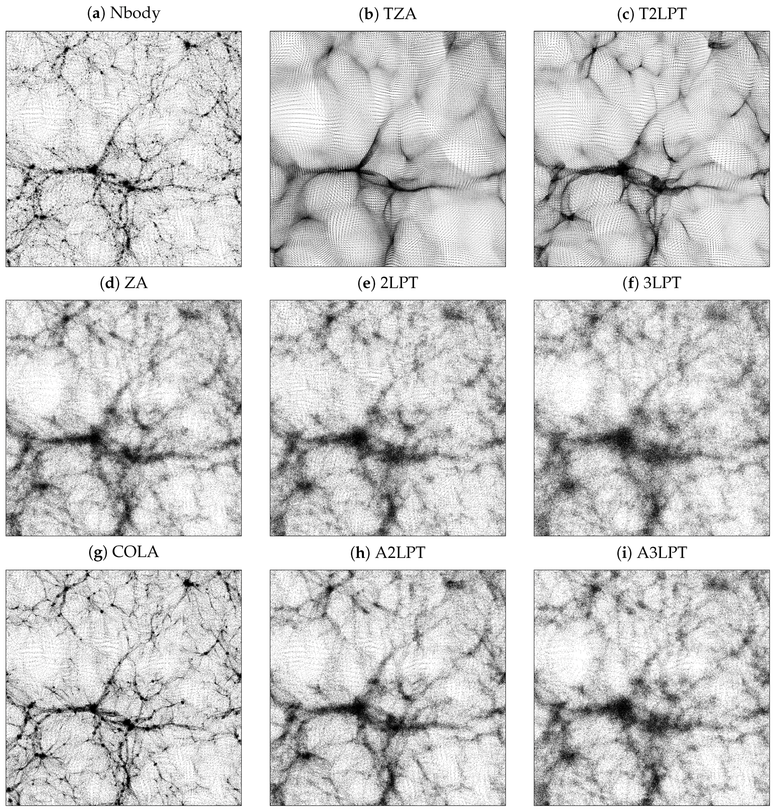
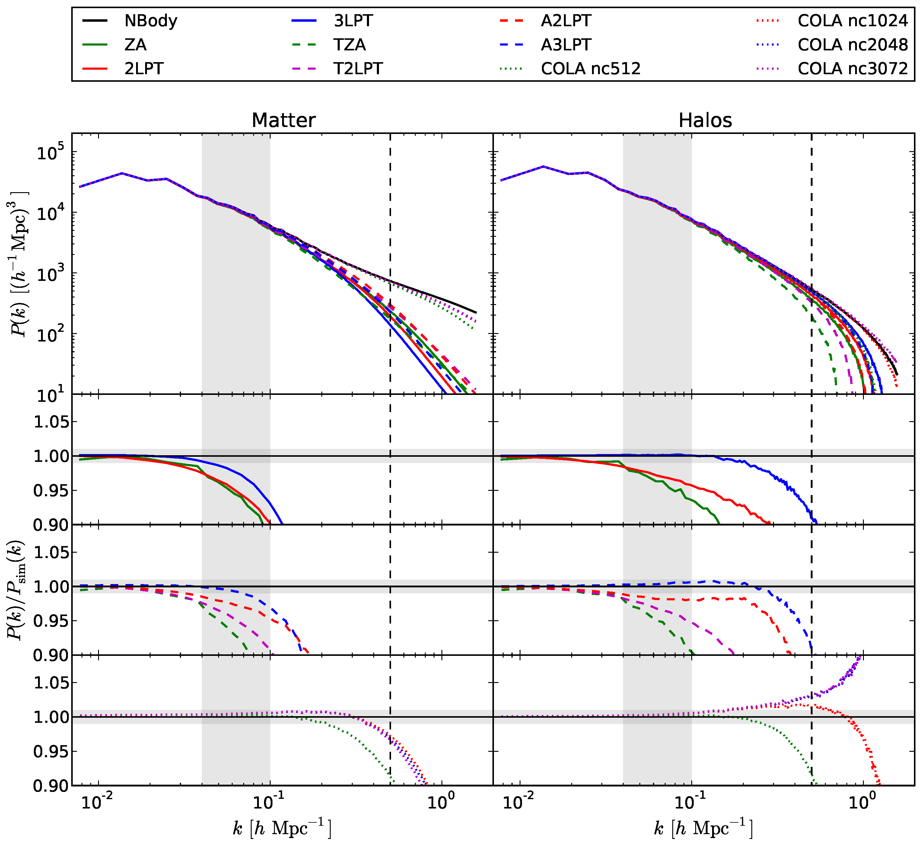
For the matter power spectrum, the wavenumber at which power drops below a $-10$% level does not overtake 0.2 h Mpc${}^{-1}$ for all models, with the exception of COLA, that can reach 0.8 h Mpc${}^{-1}$ for all meshes but the coarsest one. Moreover, going from lower to higher orders provides only some modest improvement, and this is true for all LPT flavours. This quantifies the trend, noticed in Figure 2, that higher LPT orders may give better convergence before orbit crossing, but they add to the spreading of the multi-stream region.

(2)

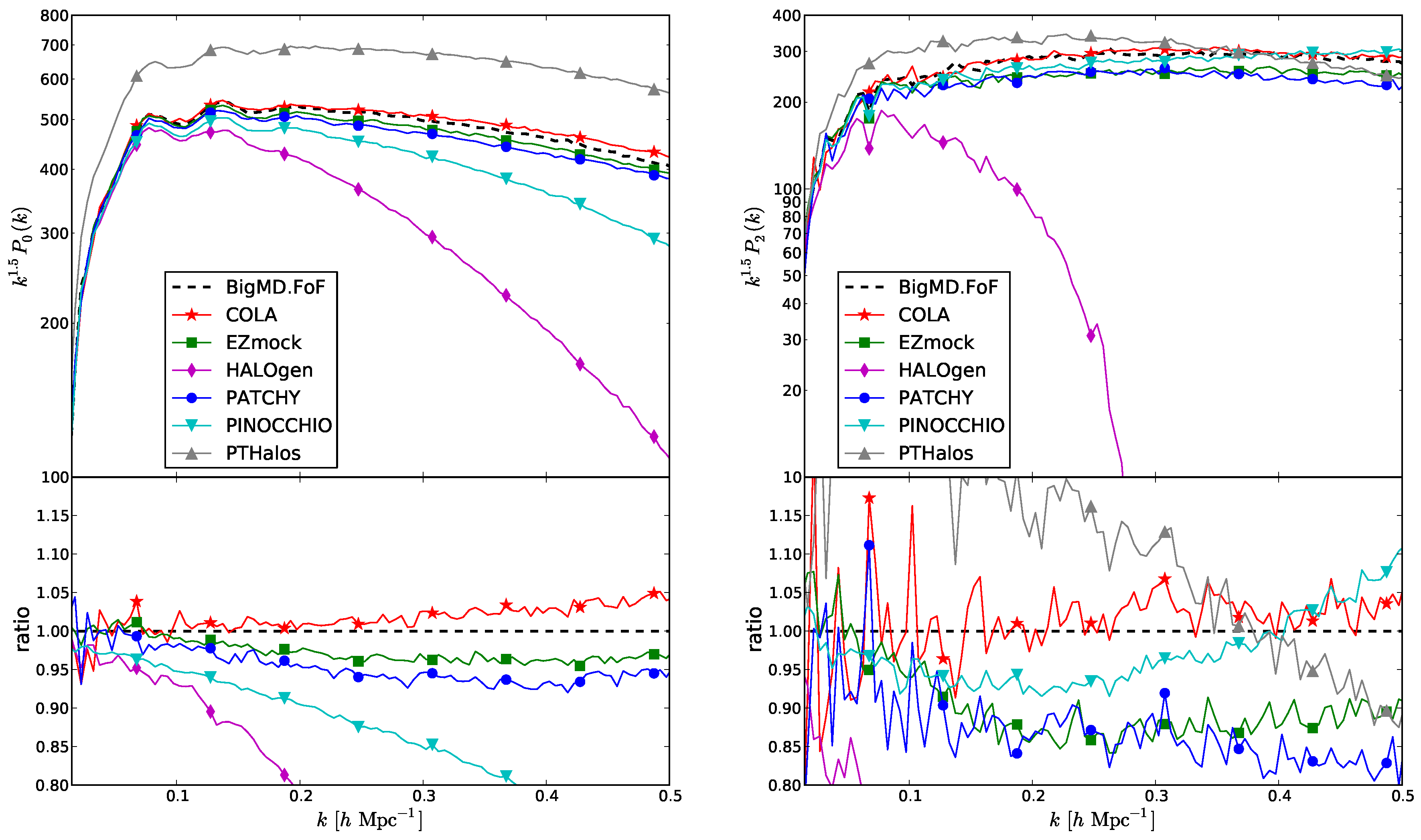
All approximate methods are able to recover the halo power spectrum at a higher wavenumber than the matter power spectrum. For the straight LPT series, power drops below a $-10$% level at k ∼0.13, $0.3$ and $0.5$ h Mpc${}^{-1}$ for the three orders, showing that the improvement achieved going to higher orders is significant.

(3)

No advantage is found by adopting the truncated LPT scheme. As noticed in Section 3.4, in the original paper of Coles et al. [102] the advantage of the truncated scheme was found to be good for a power spectrum of positive or flat slope ≥$-1$ but marginal for a slope $-2$, that is shallower than the slope of a ΛCDM spectrum at k ∼0.5.

(4)

Augmentation contributes to the improvement of the LPT series. This trend is more apparent for the halo power spectrum, in which case the improvement in going from 2LPT to A2LPT is of the same order as the improvement in going from 2LPT to 3LPT. A3LPT is only marginally better than 3LPT.

(5)

COLA gives percent accurate results for the matter power spectrum up to k ∼0.5 h Mpc${}^{-1}$, and is 10% accurate up to $k=0.8$ h Mpc${}^{-1}$. Very good results are obtained for halos, where some excess power at the 2% level is found at $k=0.5$, but 10% accuracy is achieved up to $k=1$ h Mpc${}^{-1}$. Results are stable with the grid dimension, with the exception of the coarsest grid that gives poor performance; for halos, finer grids give some excess of power, the ${1024}^3$ grid gives the best performance. Clearly, finer grids are needed by COLA to allow proper identification of halos, but not to achieve better accuracy in their clustering.

These results demonstrate the potentiality of approximate methods based on LPT to correctly place DM halos: both 3LPT and A3LPT displacements are still 10% accurate up to $k=0.5$ h Mpc${}^{-1}$, the scale at which the 1-halo term is becoming dominant, while COLA outperforms all methods even with a ${1024}^3$ grid. This is true, of course, provided that the Lagrangian part of the problem, particle assignments to halos, is solved with good accuracy.

Before going to the conclusions, I want to stress that averaging over the Lagrangian patch of a DM halo is already a form of smoothing. Recently, Kopp et al. [218] advocated the use of smoothing to improve the predictions of one extension of LPT, where their smoothing length is equal to the Lagrangian size of the halo. This “truncation” is necessary to insert the information of the Lagrangian size of a halo into an analytic formalism. So their “choose to smooth” message is not in contrast with our conclusion that truncation does not help LPT in this context.

6. Concluding Remarks

The search for analytic and semi-analytic approximations to gravitational clustering, more than being pushed out of fashion, has been boosted by precision cosmology. This is perfectly in line with the ideas laid down since the late 1960s, when the Russian school started to investigate the formation of large-scale structure, to the 1990s, when analytic approximations were systematically investigated and used to constrain the cosmological model. Indeed, the ability to understand the fine details of clustering pays off when the “blind” solution of N-body simulations must be demonstrated to be accurate to a certain level, or must be replicated a very large number of times to quantify the systematics of a galaxy survey.

One of the reasons why approximate methods are acceptable, that was pointed out by Scoccimarro and Sheth in the PTHalos presentation paper [188], is that the very non-linear baryonic processes that lead to the formation of galaxies drastically limit the possibility to accurately predict what happens on small scales, roughly where the one-halo term becomes dominant. On larger scales, uncertainties in galaxy formation mainly emerge as an uncertainty in galaxy bias, that as mentioned in Section 4.1 can be directly measured from the data using higher-order correlation and marginalized over when estimating cosmological parameters.

This review is mostly concerned with the interpretation of galaxy clustering. Galaxy weak lensing is another, very powerful tool for the clustering of matter, that has the great advantage of directly testing the gravitational potential along a line of sight. Galaxies here are not unfaithful tracers of the large-scale density field, but just background objects whose ellipticity is perturbed by gravitational lensing. The issue in this case is whether galaxy ellipticities are correlated, and to properly subtract this nuisance term. There is in principle no reason why approximate methods cannot be used to generate realizations of matter and gravitational potential distributions. However, if the use of galaxy clustering is limited to the range of scales that are dominated by the 2-halo term, k ∼0.5 h Mpc${}^{-1}$, galaxy lensing has the power to directly investigate the potential down to much smaller scales, at least to k ∼10 h Mpc${}^{-1}$. Here the details of halo structure, as ellipticity or substructure, become determinant. This issue was addressed by Pace et al. [219], who computed both the matter power spectrum and the lensing potential of an N-body simulation trying different experiments: take only particles found in halos or outside halos; use only halos to compute the density field; rotate halos to randomize their ellipticities; make halos isotropic by rotating their particles to erase substructure and ellipticity; displace halos with 2LPT. Remarkably, the removal of substructure by isotropization of halos was found to have a small impact on $P(k)$ up to $0.5$ h Mpc${}^{-1}$, but to influence the lensing angular power spectrum at $l>300$. Clearly, the assumption of spherical and smooth halos done by all mock generators does not allow to reach good accuracy. A way out may be to construct halo models that reproduce ellipticities and substructure, as done with the Matter density distributiOn Kode for gravitationAl lenses (MOKA) of Giocoli et al. [220], that was developed to make predictions on strong lensing by galaxy clusters.

Throughout this paper, I described how to produce catalogs of DM halos, but this is only the first step in the construction of a mock galaxy catalog. DM halos must be populated with galaxies, that should follow a given luminosity function, so that a flux cut can be applied to the galaxy distribution to produce a realistic mock. This step can be performed using three different techniques. Halo occupation distribution models (e.g., [221,222,223,224,225]) populate each DM halo with a number of galaxies that depends on its mass, and this dependence is obtained by requiring to reproduce the number density (or luminosity function in some cases) and correlation function of galaxies. In subhalo abundance matching models (e.g., [226,227]) the simulation is able to resolve substructures of DM halos, named sub-halos, and these are populated with galaxies assuming a one-to-one correspondence. The third class is that of SAMs of galaxy formation [31,32,33], applied to the merger trees of an N-body simulation (one example for all, [228]). Because the exact correspondence of galaxies and halos or sub-halos depends on the complex physics of galaxy formation, there can be no guarantee of accuracy in this step. Cosmological measurements will be highly accurate as long as they are not influenced much by it.

References

1. Coles, P.; Lucchin, F. Cosmology: The Origin and Evolution of Cosmic Structure, 2nd ed.; Wiley: Hoboken, NJ, USA, 2002; p. 512. [Google Scholar]
2. Mo, H.; van den Bosch, F.C.; White, S. Galaxy Formation and Evolution; Cambridge University Press: Cambridge, UK, 2010. [Google Scholar]
3. Planck Collaboration; Ade, P.A.R.; Aghanim, N.; Alves, M.I.R.; Armitage-Caplan, C.; Arnaud, M.; Ashdown, M.; Atrio-Barandela, F.; Aumont, J.; Aussel, H.; et al. Planck 2013 results. I. Overview of products and scientific results. Astron. Astrophys. 2014, 571, A1. [Google Scholar]
4. Buchert, T. Toward physical cosmology: Focus on inhomogeneous geometry and its non-perturbative effects. Class. Quantum Gravity 2011, 28, 164007. [Google Scholar] [CrossRef]
5. Springel, V. The cosmological simulation code GADGET-2. Mon. Not. R. Astron. Soc. 2005, 364, 1105–1134. [Google Scholar] [CrossRef]
6. Hockney, R.W.; Eastwood, J.W. Computer Simulation Using Particles; McGraw-Hill: New York, NY, USA, 1981. [Google Scholar]
7. Springel, V.; White, S.D.M.; Jenkins, A.; Frenk, C.S.; Yoshida, N.; Gao, L.; Navarro, J.; Thacker, R.; Croton, D.; Helly, J.; et al. Simulations of the formation, evolution and clustering of galaxies and quasars. Nature 2005, 435, 629–636. [Google Scholar] [CrossRef] [PubMed]
8. Alimi, J.M.; Bouillot, V.; Rasera, Y.; Reverdy, V.; Corasaniti, P.S.; Balmes, I.; Requena, S.; Delaruelle, X.; Richet, J.N. DEUS Full Observable ΛCDM Universe Simulation: The Numerical Challenge. 2012; arXiv:1206.2838. [Google Scholar]
9. Angulo, R.E.; Springel, V.; White, S.D.M.; Jenkins, A.; Baugh, C.M.; Frenk, C.S. Scaling relations for galaxy clusters in the Millennium-XXL simulation. Mon. Not. R. Astron. Soc. 2012, 426, 2046–2062. [Google Scholar] [CrossRef] [Green Version]
10. Watson, W.A.; Iliev, I.T.; Diego, J.M.; Gottlöber, S.; Knebe, A.; Martínez-González, E.; Yepes, G. Statistics of extreme objects in the Juropa Hubble Volume simulation. Mon. Not. R. Astron. Soc. 2014, 437, 3776–3786. [Google Scholar] [CrossRef]
11. Heitmann, K.; Frontiere, N.; Sewell, C.; Habib, S.; Pope, A.; Finkel, H.; Rizzi, S.; Insley, J.; Bhattacharya, S. The Q continuum simulation: Harnessing the power of GPU accelerated supercomputers. Astrophys. J. Suppl. 2015, 219, 34. [Google Scholar] [CrossRef]
12. Skillman, S.W.; Warren, M.S.; Turk, M.J.; Wechsler, R.H.; Holz, D.E.; Sutter, P.M. Dark Sky Simulations: Early Data Release. 2014; arXiv:1407.2600. [Google Scholar]
13. Kim, J.; Park, C.; L’Huillier, B.; Hong, S.E. Horizon Run 4 simulation: Coupled evolution of galaxies and large-scale structures of the Universe. J. Korean Astron. Soc. 2015, 48, 213–228. [Google Scholar] [CrossRef]
14. Potter, D.; Stadel, J.; Teyssier, R. PKDGRAV3: Beyond Trillion Particle Cosmological Simulations for the Next Era of Galaxy Surveys. 2016; arXiv:1609.08621. [Google Scholar]
15. Heitmann, K.; White, M.; Wagner, C.; Habib, S.; Higdon, D. The Coyote Universe. I. Precision determination of the nonlinear matter power spectrum. Astrophys. J. 2010, 715, 104–121. [Google Scholar] [CrossRef]
16. Reed, D.S.; Smith, R.E.; Potter, D.; Schneider, A.; Stadel, J.; Moore, B. Towards an accurate mass function for precision cosmology. Mon. Not. R. Astron. Soc. 2013, 431, 1866–1882. [Google Scholar] [CrossRef]
17. Schneider, A.; Teyssier, R.; Potter, D.; Stadel, J.; Onions, J.; Reed, D.S.; Smith, R.E.; Springel, V.; Pearce, F.R.; Scoccimarro, R. Matter Power Spectrum and the Challenge of Percent Accuracy. 2015; arXiv:1503.05920. [Google Scholar]
18. Lynden-Bell, D. Statistical mechanics of violent relaxation in stellar systems. Mon. Not. R. Astron. Soc. 1967, 136, 101–121. [Google Scholar] [CrossRef]
19. Saslaw, W.C. Gravitational Physics of Stellar and Galactic Systems; Cambridge University Press: Cambridge, UK, 1985. [Google Scholar]
20. Navarro, J.F.; Frenk, C.S.; White, S.D.M. The structure of cold dark matter halos. Astrophys. J. 1996, 462, 563–575. [Google Scholar] [CrossRef]
21. Hinshaw, G.; Larson, D.; Komatsu, E.; Spergel, D.N.; Bennett, C.L.; Dunkley, J.; Nolta, M.R.; Halpern, M.; Hill, R.S.; Odegard, N.; et al. Nine-year Wilkinson Microwave Anisotropy Probe (WMAP) observations: Cosmological parameter results. Astrophys. J. Suppl. 2013, 208, 19. [Google Scholar] [CrossRef]
22. Planck Collaboration; Ade, P.A.R.; Aghanim, N.; Arnaud, M.; Ashdown, M.; Aumont, J.; Baccigalupi, C.; Banday, A.J.; Barreiro, R.B.; Bartlett, J.G.; et al. Planck 2015 Results. XIII. Cosmological Parameters. 2015; arXiv:1502.01589. [Google Scholar]
23. Frieman, J. Dark Energy Survey Collaboration. In Proceedings of the 221th Meeting of the American Astronomical Society, Long Beach, CA, USA, 6–10 January 2013.
24. Dawson, K.S.; Kneib, J.P.; Percival, W.J.; Alam, S.; Albareti, F.D.; Anderson, S.F.; Armengaud, E.; Aubourg, É.; Bailey, S.; Bautista, J.E.; et al. The SDSS-IV extended baryon oscillation spectroscopic survey: Overview and early data. Astron. J. 2016, 151, 44. [Google Scholar] [CrossRef] [Green Version]
25. Levi, M.; Bebek, C.; Beers, T.; Blum, R.; Cahn, R.; Eisenstein, D.; Flaugher, B.; Honscheid, K.; Kron, R.; Lahav, O.; et al. The DESI Experiment, a Whitepaper for Snowmass 2013. 2013; arXiv:1308.0847. [Google Scholar]
26. LSST Science Collaboration; Abell, P.A.; Allison, J.; Anderson, S.F.; Andrew, J.R.; Angel, J.R.P.; Armus, L.; Arnett, D.; Asztalos, S.J.; Axelrod, T.S.; et al. LSST Science Book. Version 2.0. 2009; arXiv:0912.0201. [Google Scholar]
27. Laureijs, R.; Amiaux, J.; Arduini, S.; Auguères, J.; Brinchmann, J.; Cole, R.; Cropper, M.; Dabin, C.; Duvet, L.; Ealet, A.; et al. Euclid Definition Study Report. 2011; arXiv:1110.3193. [Google Scholar]
28. Green, J.; Schechter, P.; Baltay, C.; Bean, R.; Bennett, D.; Brown, R.; Conselice, C.; Donahue, M.; Fan, X.; Gaudi, B.S.; et al. Wide-Field InfraRed Survey Telescope (WFIRST) Final Report. 2012; arXiv:1208.4012. [Google Scholar]
29. Kitaura, F.S.; Enßlin, T.A. Bayesian reconstruction of the cosmological large-scale structure: Methodology, inverse algorithms and numerical optimization. Mon. Not. R. Astron. Soc. 2008, 389, 497–544. [Google Scholar] [CrossRef]
30. Jasche, J.; Kitaura, F.S.; Wandelt, B.D.; Enßlin, T.A. Bayesian power-spectrum inference for large-scale structure data. Mon. Not. R. Astron. Soc. 2010, 406, 60–85. [Google Scholar] [CrossRef]
31. Baugh, C.M. A primer on hierarchical galaxy formation: the semi-analytical approach. Rep. Prog. Phys. 2006, 69, 3101–3156. [Google Scholar] [CrossRef]
32. Benson, A.J. Galaxy formation theory. Phys. Rep. 2010, 495, 33–86. [Google Scholar] [CrossRef]
33. Somerville, R.S.; Davé, R. Physical models of galaxy formation in a cosmological framework. Ann. Rev. Astron. Astrophys. 2015, 53, 51–113. [Google Scholar] [CrossRef]
34. Peebles, P.J.E. The Large-Scale Structure of the Universe; Princeton University Press: Princeton, NJ, USA, 1980. [Google Scholar]
35. Buchert, T.; Ehlers, J. Averaging inhomogeneous Newtonian cosmologies. Astron. Astrophys. 1997, 320, 1–7. [Google Scholar]
36. Bernardeau, F.; Colombi, S.; Gaztañaga, E.; Scoccimarro, R. Large-scale structure of the Universe and cosmological perturbation theory. Phys. Rep. 2002, 367, 1–248. [Google Scholar] [CrossRef]
37. Carlson, J.; White, M.; Padmanabhan, N. Critical look at cosmological perturbation theory techniques. Phys. Rev. D 2009, 80, 043531. [Google Scholar] [CrossRef]
38. Zel’dovich, Y.B. Gravitational instability: An approximate theory for large density perturbations. Astron. Astrophys. 1970, 5, 84–89. [Google Scholar]
39. Shandarin, S.F.; Zeldovich, Y.B. The large-scale structure of the universe: Turbulence, intermittency, structures in a self-gravitating medium. Rev. Mod. Phys. 1989, 61, 185–220. [Google Scholar] [CrossRef]
40. Buchert, T. A class of solutions in Newtonian cosmology and the pancake theory. Astron. Astrophys. 1989, 223, 9–24. [Google Scholar]
41. Moutarde, F.; Alimi, J.M.; Bouchet, F.R.; Pellat, R.; Ramani, A. Precollapse scale invariance in gravitational instability. Astrophys. J. 1991, 382, 377–381. [Google Scholar] [CrossRef]
42. Bouchet, F.R.; Juszkiewicz, R.; Colombi, S.; Pellat, R. Weakly nonlinear gravitational instability for arbitrary Omega. Astrophys. J. Lett. 1992, 394, L5–L8. [Google Scholar] [CrossRef]
43. Bouchet, F.R.; Colombi, S.; Hivon, E.; Juszkiewicz, R. Perturbative Lagrangian approach to gravitational instability. Astron. Astrophys. 1995, 296, 575. [Google Scholar]
44. Buchert, T. Lagrangian theory of gravitational instability of Friedman-Lemaitre cosmologies and the ‘Zel’dovich approximation’. Mon. Not. R. Astron. Soc. 1992, 254, 729–737. [Google Scholar] [CrossRef]
45. Buchert, T.; Ehlers, J. Lagrangian theory of gravitational instability of Friedman-Lemaitre cosmologies—Second-order approach: An improved model for non-linear clustering. Mon. Not. R. Astron. Soc. 1993, 264, 375–387. [Google Scholar] [CrossRef]
46. Buchert, T. Lagrangian theory of gravitational instability of Friedman-Lemaitre cosmologies—A generic third-order model for nonlinear clustering. Mon. Not. R. Astron. Soc. 1994, 267, 811–820. [Google Scholar] [CrossRef]
47. Buchert, T. Lagrangian perturbation theory—A key-model for large-scale structure. Astron. Astrophys. 1993, 267, L51–L54. [Google Scholar]
48. Catelan, P. Lagrangian dynamics in non-flat universes and non-linear gravitational evolution. Mon. Not. R. Astron. Soc. 1995, 276, 115–124. [Google Scholar]
49. Buchert, T. Lagrangian perturbation approach to the formation of large-scale structure. In Dark Matter in the Universe; Bonometto, S., Primack, J.R., Provenzale, A., Eds.; IOS Press: Amsterdam, The Netherlands, 1996. [Google Scholar]
50. Bouchet, F.R. Introductory overview of eulerian and Lagrangian perturbation theories. In Dark Matter in the Universe; Bonometto, S., Primack, J.R., Provenzale, A., Eds.; IOS Press: Amsterdam, The Netherlands, 1996; p. 565. [Google Scholar]
51. Ehlers, J.; Buchert, T. Newtonian cosmology in Lagrangian formulation: Foundations and perturbation theory. Gen. Relativ. Gravit. 1997, 29, 733–764. [Google Scholar] [CrossRef]
52. Crocce, M.; Pueblas, S.; Scoccimarro, R. Transients from initial conditions in cosmological simulations. Mon. Not. R. Astron. Soc. 2006, 373, 369–381. [Google Scholar] [CrossRef]
53. Scoccimarro, R. Transients from initial conditions: A perturbative analysis. Mon. Not. R. Astron. Soc. 1998, 299, 1097–1118. [Google Scholar] [CrossRef]
54. Angulo, R.E.; Hahn, O.; Ludlow, A.; Bonoli, S. Earth-Mass Haloes and the Emergence of NFW Density Profiles. 2016; arXiv:1604.03131. [Google Scholar]
55. Ishiyama, T. Hierarchical formation of dark matter halos and the free streaming scale. Astrophys. J. 2014, 788, 27. [Google Scholar] [CrossRef]
56. Press, W.H.; Schechter, P. Formation of galaxies and clusters of galaxies by self-similar gravitational condensation. Astrophys. J. 1974, 187, 425–438. [Google Scholar] [CrossRef]
57. Doroshkevich, A.G. Momentum and mass distribution funcatons for newly generated cosmic objects. Astrophysics 1967, 3, 175–188. [Google Scholar] [CrossRef]
58. Efstathiou, G.; Frenk, C.S.; White, S.D.M.; Davis, M. Gravitational clustering from scale-free initial conditions. Mon. Not. R. Astron. Soc. 1988, 235, 715–748. [Google Scholar] [CrossRef]
59. Epstein, R.I. Proto-galactic perturbations. Mon. Not. R. Astron. Soc. 1983, 205, 207–229. [Google Scholar] [CrossRef]
60. Peacock, J.A.; Heavens, A.F. Alternatives to the Press-Schechter cosmological mass function. Mon. Not. R. Astron. Soc. 1990, 243, 133–143. [Google Scholar] [CrossRef]
61. Bond, J.R.; Cole, S.; Efstathiou, G.; Kaiser, N. Excursion set mass functions for hierarchical Gaussian fluctuations. Astrophys. J. 1991, 379, 440–460. [Google Scholar] [CrossRef]
62. Monaco, P. The Cosmological Mass Function. Fundam. Cosm. Phys. 2008, 19, 157–317. [Google Scholar]
63. Zentner, A.R. The excursion set theory of halo mass functions, halo clustering, and halo growth. Int. J. Mod. Phys. D 2007, 16, 763–816. [Google Scholar] [CrossRef]
64. Bower, R.G. The evolution of groups of galaxies in the Press-Schechter formalism. Mon. Not. R. Astron. Soc. 1991, 248, 332–352. [Google Scholar] [CrossRef]
65. Lacey, C.; Cole, S. Merger rates in hierarchical models of galaxy formation. Mon. Not. R. Astron. Soc. 1993, 262, 627–649. [Google Scholar] [CrossRef]
66. Sheth, R.K.; Lemson, G. The forest of merger history trees associated with the formation of dark matter haloes. Mon. Not. R. Astron. Soc. 1999, 305, 946–956. [Google Scholar] [CrossRef]
67. Somerville, R.S.; Kolatt, T.S. How to plant a merger tree. Mon. Not. R. Astron. Soc. 1999, 305, 1–14. [Google Scholar] [CrossRef]
68. Van den Bosch, F.C. The universal mass accretion history of cold dark matter haloes. Mon. Not. R. Astron. Soc. 2002, 331, 98–110. [Google Scholar] [CrossRef]
69. Sheth, R.K.; Tormen, G. Large-scale bias and the peak background split. Mon. Not. R. Astron. Soc. 1999, 308, 119–126. [Google Scholar] [CrossRef]
70. Sheth, R.K.; Tormen, G. An excursion set model of hierarchical clustering: Ellipsoidal collapse and the moving barrier. Mon. Not. R. Astron. Soc. 2002, 329, 61–75. [Google Scholar] [CrossRef]
71. Monaco, P. Dynamics in the Cosmological Mass Function (or, why does the Press & Schechter work?). In Observational Cosmology: The Development of Galaxy Systems; Giuricin, G., Mezzetti, M., Salucci, P., Eds.; Astronomical Society of the Pacific Conference Series; Astronomical Society of the Pacific: San Francisco, CA, USA, 1999; Volume 176, p. 186. [Google Scholar]
72. Sheth, R.K. Random walks and the additive coagulation equation. Mon. Not. R. Astron. Soc. 1998, 295, 869–872. [Google Scholar] [CrossRef]
73. Adler, R.J. The Geometry of Random Fields; SIAM-Society for Industrial and Applied Mathematics: Philadelphia, PA, USA, 1981. [Google Scholar]
74. Doroshkevich, A.G. The space structure of perturbations and the origin of rotation of galaxies in the theory of fluctuation. Astrofizika 1970, 6, 591–600. [Google Scholar]
75. Peacock, J.A.; Heavens, A.F. The statistics of maxima in primordial density perturbations. Mon. Not. R. Astron. Soc. 1985, 217, 805–820. [Google Scholar] [CrossRef]
76. Bardeen, J.M.; Bond, J.R.; Kaiser, N.; Szalay, A.S. The statistics of peaks of Gaussian random fields. Astrophys. J. 1986, 304, 15–61. [Google Scholar] [CrossRef]
77. Kerscher, M.; Buchert, T.; Futamase, T. On the abundance of collapsed objects. Astrophys. J. Lett. 2001, 558, L79–L82. [Google Scholar] [CrossRef] [Green Version]
78. Bond, J.R.; Myers, S.T. The peak-patch picture of cosmic catalogs. I. Algorithms. Astrophys. J. Suppl. 1996, 103, 1. [Google Scholar] [CrossRef]
79. Nadkarni-Ghosh, S.; Singhal, A. Phase space dynamics of triaxial collapse: Joint density-velocity evolution. Mon. Not. R. Astron. Soc. 2016, 457, 2773–2789. [Google Scholar] [CrossRef]
80. Monaco, P. The mass function of cosmic structures with nonspherical collapse. Astrophys. J. 1995, 447, 23. [Google Scholar] [CrossRef]
81. Monaco, P. A Lagrangian dynamical theory for the mass function of cosmic structures—I. Dynamics. Mon. Not. R. Astron. Soc. 1997, 287, 753–770. [Google Scholar] [CrossRef]
82. Hahn, O.; Porciani, C.; Carollo, C.M.; Dekel, A. Properties of dark matter haloes in clusters, filaments, sheets and voids. Mon. Not. R. Astron. Soc. 2007, 375, 489–499. [Google Scholar] [CrossRef]
83. Cooray, A.; Sheth, R. Halo models of large scale structure. Phys. Rep. 2002, 372, 1–129. [Google Scholar] [CrossRef]
84. Kaiser, N. On the spatial correlations of Abell clusters. Astrophys. J. Lett. 1984, 284, L9–L12. [Google Scholar] [CrossRef]
85. Bagla, J.S. Evolution of galaxy clustering. Mon. Not. R. Astron. Soc. 1998, 299, 417–424. [Google Scholar] [CrossRef]
86. Mo, H.J.; White, S.D.M. An analytic model for the spatial clustering of dark matter haloes. Mon. Not. R. Astron. Soc. 1996, 282, 347–361. [Google Scholar] [CrossRef]
87. Sheth, R.K.; Mo, H.J.; Tormen, G. Ellipsoidal collapse and an improved model for the number and spatial distribution of dark matter haloes. Mon. Not. R. Astron. Soc. 2001, 323, 1–12. [Google Scholar] [CrossRef]
88. Jing, Y.P. Accurate fitting formula for the two-point correlation function of dark matter halos. Astrophys. J. Lett. 1998, 503, L9–L13. [Google Scholar] [CrossRef]
89. Fry, J.N.; Gaztanaga, E. Biasing and hierarchical statistics in large-scale structure. Astrophys. J. 1993, 413, 447–452. [Google Scholar] [CrossRef]
90. Chan, K.C.; Scoccimarro, R.; Sheth, R.K. Gravity and large-scale nonlocal bias. Phys. Rev. D 2012, 85, 083509. [Google Scholar] [CrossRef]
91. Sheth, R.K.; Chan, K.C.; Scoccimarro, R. Nonlocal Lagrangian bias. Phys. Rev. D 2013, 87, 083002. [Google Scholar] [CrossRef]
92. Dekel, A.; Lahav, O. Stochastic nonlinear galaxy biasing. Astrophys. J. 1999, 520, 24–34. [Google Scholar] [CrossRef]
93. Sahni, V.; Coles, P. Approximation methods for non-linear gravitational clustering. Phys. Rep. 1995, 262, 1–135. [Google Scholar] [CrossRef]
94. Coles, P.; Jones, B. A lognormal model for the cosmological mass distribution. Mon. Not. R. Astron. Soc. 1991, 248, 1–13. [Google Scholar] [CrossRef]
95. Kofman, L.A.; Shandarin, S.F. Theory of adhesion for the large-scale structure of the universe. Nature 1988, 334, 129–131. [Google Scholar] [CrossRef]
96. Gurbatov, S.N.; Saichev, A.I.; Shandarin, S.F. The large-scale structure of the universe in the frame of the model equation of non-linear diffusion. Mon. Not. R. Astron. Soc. 1989, 236, 385–402. [Google Scholar] [CrossRef]
97. Kofman, L.; Pogosyan, D.; Shandarin, S.F.; Melott, A.L. Coherent structures in the universe and the adhesion model. Astrophys. J. 1992, 393, 437–449. [Google Scholar] [CrossRef]
98. Buchert, T.; Dominguez, A. Modeling multi-stream flow in collisionless matter: Approximations for large-scale structure beyond shell-crossing. Astron. Astrophys. 1998, 335, 395–402. [Google Scholar]
99. Menci, N. An Eulerian perturbation approach to large-scale structures: Extending the adhesion approximation. Mon. Not. R. Astron. Soc. 2002, 330, 907–919. [Google Scholar] [CrossRef]
100. Matarrese, S.; Lucchin, F.; Moscardini, L.; Saez, D. A frozen-flow approximation to the evolution of large-scale structures in the Universe. Mon. Not. R. Astron. Soc. 1992, 259, 437–452. [Google Scholar] [CrossRef]
101. Bagla, J.S.; Padmanabhan, T. Nonlinear evolution of density perturbations using the approximate constancy of the gravitational potential. Mon. Not. R. Astron. Soc. 1994, 266, 227. [Google Scholar] [CrossRef]
102. Coles, P.; Melott, A.L.; Shandarin, S.F. Testing approximations for non-linear gravitational clustering. Mon. Not. R. Astron. Soc. 1993, 260, 765–776. [Google Scholar] [CrossRef]
103. Melott, A.L.; Buchert, T.; Weib, A.G. Testing higher-order Lagrangian perturbation theory against numerical simulations. 2: Hierarchical models. Astron. Astrophys. 1995, 294, 345–365. [Google Scholar]
104. Melott, A.L. Comparison of dynamical approximation schemes for nonlinear gravitaional clustering. Astrophys. J. Lett. 1994, 426, L19–L22. [Google Scholar] [CrossRef]
105. Borgani, S.; Coles, P.; Moscardini, L. Cluster correlations in the Zel’dovich approximation. Mon. Not. R. Astron. Soc. 1994, 271, 223. [Google Scholar] [CrossRef]
106. Nusser, A.; Dekel, A. Tracing large-scale fluctuations back in time. Astrophys. J. 1992, 391, 443–452. [Google Scholar] [CrossRef]
107. Peebles, P.J.E. Tracing galaxy orbits back in time. Astrophys. J. Lett. 1989, 344, L53–L56. [Google Scholar] [CrossRef]
108. Keselman, A.; Nusser, A. Performance Study of Lagrangian Methods: Reconstruction of Large Scale Peculiar Velocities and Baryonic Acoustic Oscillations. 2016; arXiv:1609.03576. [Google Scholar]
109. Monaco, P.; Efstathiou, G. Reconstruction of cosmological initial conditions from galaxy redshift catalogues. Mon. Not. R. Astron. Soc. 1999, 308, 763–779. [Google Scholar] [CrossRef]
110. Mohayaee, R.; Mathis, H.; Colombi, S.; Silk, J. Reconstruction of primordial density fields. Mon. Not. R. Astron. Soc. 2006, 365, 939–959. [Google Scholar] [CrossRef]
111. Mohayaee, R.; Frisch, U.; Matarrese, S.; Sobolevskii, A. Back to the primordial Universe by a Monge-Ampère-Kantorovich optimization scheme. Astron. Astrophys. 2003, 406, 393–401. [Google Scholar] [CrossRef]
112. Hoffman, Y.; Ribak, E. Constrained realizations of Gaussian fields—A simple algorithm. Astrophys. J. Lett. 1991, 380, L5–L8. [Google Scholar] [CrossRef]
113. L’Huillier, B.; Park, C.; Kim, J. Effects of the initial conditions on cosmological N-body simulations. New Astron. 2014, 30, 79–88. [Google Scholar] [CrossRef]
114. Garrison, L.H.; Eisenstein, D.J.; Ferrer, D.; Metchnik, M.V.; Pinto, P.A. Improving Initial Conditions for Cosmological N-Body Simulations. 2016; arXiv:1605.02333. [Google Scholar]
115. Pope, A.C.; Szapudi, I. Shrinkage estimation of the power spectrum covariance matrix. Mon. Not. R. Astron. Soc. 2008, 389, 766–774. [Google Scholar] [CrossRef]
116. Schneider, M.D.; Cole, S.; Frenk, C.S.; Szapudi, I. Fast generation of ensembles of cosmological n-body simulations via mode resampling. Astrophys. J. 2011, 737, 11. [Google Scholar] [CrossRef]
117. Percival, W.J.; Ross, A.J.; Sánchez, A.G.; Samushia, L.; Burden, A.; Crittenden, R.; Cuesta, A.J.; Magana, M.V.; Manera, M.; Beutler, F.; et al. The clustering of Galaxies in the SDSS-III Baryon Oscillation Spectroscopic Survey: Including covariance matrix errors. Mon. Not. R. Astron. Soc. 2014, 439, 2531–2541. [Google Scholar] [CrossRef]
118. Paz, D.J.; Sánchez, A.G. Improving the precision matrix for precision cosmology. Mon. Not. R. Astron. Soc. 2015, 454, 4326–4334. [Google Scholar] [CrossRef]
119. Kalus, B.; Percival, W.J.; Samushia, L. Cosmological parameter inference from galaxy clustering: The effect of the posterior distribution of the power spectrum. Mon. Not. R. Astron. Soc. 2016, 455, 2573–2581. [Google Scholar] [CrossRef] [Green Version]
120. Pearson, D.W.; Samushia, L. Estimating the power spectrum covariance matrix with fewer mock samples. Mon. Not. R. Astron. Soc. 2016, 457, 993–999. [Google Scholar] [CrossRef]
121. O’Connell, R.; Eisenstein, D.; Vargas, M.; Ho, S.; Padmanabhan, N. Large Covariance Matrices: Smooth Models from the 2-Point Correlation Function. 2015; arXiv:1510.01740. [Google Scholar]
122. Padmanabhan, N.; White, M.; Zhou, H.H.; O’Connell, R. Estimating Sparse Precision Matrices. 2015; arXiv:1512.01241. [Google Scholar]
123. Angulo, R.E.; Pontzen, A. Cosmological N-body simulations with suppressed variance. Mon. Not. R. Astron. Soc. 2016, 462, L1–L5. [Google Scholar] [CrossRef]
124. Schäfer, J.; Strimmer, K. A Shrinkage approach to large-scale covariance matrix estimation and implications for functional genomics. Stat. Appl. Genet. Mol. Biol. 2005, 4, 32. [Google Scholar] [CrossRef] [PubMed]
125. De la Torre, S.; Guzzo, L.; Peacock, J.A.; Branchini, E.; Iovino, A.; Granett, B.R.; Abbas, U.; Adami, C.; Arnouts, S.; Bel, J.; et al. The VIMOS Public Extragalactic Redshift Survey (VIPERS). Galaxy clustering and redshift-space distortions at z ∼ 0.8 in the first data release. Astron. Astrophys. 2013, 557, A54. [Google Scholar] [CrossRef]
126. White, M. The Zel’dovich approximation. Mon. Not. R. Astron. Soc. 2014, 439, 3630–3640. [Google Scholar] [CrossRef]
127. White, M. Reconstruction within the Zeldovich approximation. Mon. Not. R. Astron. Soc. 2015, 450, 3822–3828. [Google Scholar] [CrossRef]
128. Eisenstein, D.J.; Seo, H.J.; Sirko, E.; Spergel, D.N. Improving cosmological distance measurements by reconstruction of the baryon acoustic peak. Astrophys. J. 2007, 664, 675–679. [Google Scholar] [CrossRef]
129. Padmanabhan, N.; White, M.; Cohn, J.D. Reconstructing baryon oscillations: A Lagrangian theory perspective. Phys. Rev. D 2009, 79, 063523. [Google Scholar] [CrossRef]
130. Padmanabhan, N.; Xu, X.; Eisenstein, D.J.; Scalzo, R.; Cuesta, A.J.; Mehta, K.T.; Kazin, E. A 2 per cent distance to z = 0.35 by reconstructing baryon acoustic oscillations—I. Methods and application to the Sloan Digital Sky Survey. Mon. Not. R. Astron. Soc. 2012, 427, 2132–2145. [Google Scholar] [CrossRef]
131. Burden, A.; Percival, W.J.; Howlett, C. Reconstruction in Fourier space. Mon. Not. R. Astron. Soc. 2015, 453, 456–468. [Google Scholar] [CrossRef] [Green Version]
132. McCullagh, N.; Szalay, A.S. Nonlinear behavior of Baryon Acoustic Oscillations from the Zel’dovich approximation using a non-fourier perturbation approach. Astrophys. J. 2012, 752, 21. [Google Scholar] [CrossRef]
133. Rampf, C.; Buchert, T. Lagrangian perturbations and the matter bispectrum I: Fourth-order model for non-linear clustering. J. Cosmol. Astropart. Phys. 2012, 6, 021. [Google Scholar] [CrossRef]
134. Tatekawa, T. Fourth-order perturbative equations in Lagrangian perturbation theory for a cosmological dust fluid. Prog. Theor. Exp. Phys. 2013, 2013, 013E03. [Google Scholar] [CrossRef]
135. Leclercq, F.; Jasche, J.; Gil-Marín, H.; Wandelt, B. One-point remapping of Lagrangian perturbation theory in the mildly non-linear regime of cosmic structure formation. J. Cosmol. Astropart. Phys. 2013, 11, 048. [Google Scholar] [CrossRef]
136. Nadkarni-Ghosh, S.; Chernoff, D.F. Modelling non-linear evolution using Lagrangian perturbation theory re-expansions. Mon. Not. R. Astron. Soc. 2013, 431, 799–823. [Google Scholar] [CrossRef]
137. Bartelmann, M. Trajectories of point particles in cosmology and the Zel’dovich approximation. Phys. Rev. D 2015, 91, 083524. [Google Scholar] [CrossRef]
138. Tassev, S. Lagrangian or Eulerian; real or Fourier? Not all approaches to large-scale structure are created equal. J. Cosmol. Astropart. Phys. 2014, 6, 008. [Google Scholar] [CrossRef] [PubMed]
139. Sugiyama, N.S. Using Lagrangian perturbation theory for precision cosmology. Astrophys. J. 2014, 788, 63. [Google Scholar] [CrossRef]
140. Vlah, Z.; Seljak, U.; Baldauf, T. Lagrangian perturbation theory at one loop order: Successes, failures, and improvements. Phys. Rev. D 2015, 91, 023508. [Google Scholar] [CrossRef]
141. Carrasco, J.J.M.; Hertzberg, M.P.; Senatore, L. The effective field theory of cosmological large scale structures. J. High Energy Phys. 2012, 9, 82. [Google Scholar] [CrossRef]
142. Porto, R.A.; Senatore, L.; Zaldarriaga, M. The Lagrangian-space Effective Field Theory of large scale structures. J. Cosmol. Astropart. Phys. 2014, 5, 022. [Google Scholar] [CrossRef]
143. Baldauf, T.; Schaan, E.; Zaldarriaga, M. On the reach of perturbative methods for dark matter density fields. J. Cosmol. Astropart. Phys. 2016, 3, 007. [Google Scholar] [CrossRef] [PubMed]
144. Kitaura, F.S.; Heß, S. Cosmological structure formation with augmented Lagrangian perturbation theory. Mon. Not. R. Astron. Soc. 2013, 435, L78–L82. [Google Scholar] [CrossRef]
145. Bernardeau, F. The nonlinear evolution of rare events. Astrophys. J. 1994, 427, 51–71. [Google Scholar] [CrossRef]
146. Neyrinck, M.C. Quantifying distortions of the Lagrangian dark-matter mesh in cosmology. Mon. Not. R. Astron. Soc. 2013, 428, 141–153. [Google Scholar] [CrossRef]
147. Chan, K.C. Helmholtz decomposition of the Lagrangian displacement. Phys. Rev. D 2014, 89, 083515. [Google Scholar] [CrossRef]
148. Neyrinck, M.C. Truthing the stretch: Non-perturbative cosmological realizations with multiscale spherical collapse. Mon. Not. R. Astron. Soc. 2016, 455, L11–L15. [Google Scholar] [CrossRef]
149. Cole, S.; Helly, J.; Frenk, C.S.; Parkinson, H. The statistical properties of Λ cold dark matter halo formation. Mon. Not. R. Astron. Soc. 2008, 383, 546–556. [Google Scholar] [CrossRef]
150. Parkinson, H.; Cole, S.; Helly, J. Generating dark matter halo merger trees. Mon. Not. R. Astron. Soc. 2008, 383, 557–564. [Google Scholar] [CrossRef] [Green Version]
151. Maggiore, M.; Riotto, A. The halo mass function from excursion set theory. I. Gaussian fluctuations with non-markovian dependence on the smoothing scale. Astrophys. J. 2010, 711, 907–927. [Google Scholar] [CrossRef]
152. Maggiore, M.; Riotto, A. The Halo mass function from Excursion Set Theory. II. The Diffusing Barrier. Astrophys. J. 2010, 717, 515–525. [Google Scholar] [CrossRef]
153. Farahi, A.; Benson, A.J. Excursion set theory for correlated random walks. Mon. Not. R. Astron. Soc. 2013, 433, 3428–3439. [Google Scholar] [CrossRef]
154. Manrique, A.; Salvador-Sole, E. The confluent system formalism. I. The mass function of objects in the peak model. Astrophys. J. 1995, 453, 6. [Google Scholar] [CrossRef]
155. Juan, E.; Salvador-Solé, E.; Domènech, G.; Manrique, A. Fixing a rigorous formalism for the accurate analytic derivation of halo properties. Mon. Not. R. Astron. Soc. 2014, 439, 719–724. [Google Scholar] [CrossRef]
156. Paranjape, A.; Sheth, R.K. Peaks theory and the excursion set approach. Mon. Not. R. Astron. Soc. 2012, 426, 2789–2796. [Google Scholar] [CrossRef]
157. Paranjape, A.; Sheth, R.K.; Desjacques, V. Excursion set peaks: A self-consistent model of dark halo abundances and clustering. Mon. Not. R. Astron. Soc. 2013, 431, 1503–1512. [Google Scholar] [CrossRef]
158. Musso, M.; Sheth, R.K. One step beyond: The excursion set approach with correlated steps. Mon. Not. R. Astron. Soc. 2012, 423, L102–L106. [Google Scholar] [CrossRef]
159. Paranjape, A.; Sefusatti, E.; Chan, K.C.; Desjacques, V.; Monaco, P.; Sheth, R.K. Bias deconstructed: Unravelling the scale dependence of halo bias using real-space measurements. Mon. Not. R. Astron. Soc. 2013, 436, 449–459. [Google Scholar] [CrossRef]
160. Ludlow, A.D.; Borzyszkowski, M.; Porciani, C. The formation of CDM haloes—I. Collapse thresholds and the ellipsoidal collapse model. Mon. Not. R. Astron. Soc. 2014, 445, 4110–4123. [Google Scholar] [CrossRef]
161. Borzyszkowski, M.; Ludlow, A.D.; Porciani, C. The formation of cold dark matter haloes—II. Collapse time and tides. Mon. Not. R. Astron. Soc. 2014, 445, 4124–4136. [Google Scholar] [CrossRef]
162. Baldauf, T.; Seljak, U.; Senatore, L.; Zaldarriaga, M. Galaxy bias and non-linear structure formation in general relativity. J. Cosmol. Astropart. Phys. 2011, 10, 031. [Google Scholar] [CrossRef]
163. McDonald, P. Clustering of dark matter tracers: Renormalizing the bias parameters. Phys. Rev. D 2006, 74, 103512. [Google Scholar] [CrossRef]
164. Gil-Marín, H.; Verde, L.; Noreña, J.; Cuesta, A.J.; Samushia, L.; Percival, W.J.; Wagner, C.; Manera, M.; Schneider, D.P. The power spectrum and bispectrum of SDSS DR11 BOSS galaxies—II. Cosmological interpretation. Mon. Not. R. Astron. Soc. 2015, 452, 1914–1921. [Google Scholar] [CrossRef]
165. Kitaura, F.S. The initial conditions of the Universe from constrained simulations. Mon. Not. R. Astron. Soc. 2013, 429, L84–L88. [Google Scholar] [CrossRef]
166. Kitaura, F.S.; Erdoǧdu, P.; Nuza, S.E.; Khalatyan, A.; Angulo, R.E.; Hoffman, Y.; Gottlöber, S. Cosmic structure and dynamics of the local Universe. Mon. Not. R. Astron. Soc. 2012, 427, L35–L39. [Google Scholar] [CrossRef]
167. Wang, H.; Mo, H.J.; Yang, X.; Jing, Y.P.; Lin, W.P. ELUCID—Exploring the Local Universe with the Reconstructed Initial Density Field. I. Hamiltonian Markov Chain Monte Carlo Method with Particle Mesh Dynamics. Astrophys. J. 2014, 794, 94. [Google Scholar] [CrossRef]
168. Jasche, J.; Wandelt, B.D. Bayesian physical reconstruction of initial conditions from large-scale structure surveys. Mon. Not. R. Astron. Soc. 2013, 432, 894–913. [Google Scholar] [CrossRef]
169. Jasche, J.; Leclercq, F.; Wandelt, B.D. Past and present cosmic structure in the SDSS DR7 main sample. J. Cosmol. Astropart. Phys. 2015, 1, 036. [Google Scholar] [CrossRef]
170. Gottloeber, S.; Hoffman, Y.; Yepes, G. Constrained Local UniversE Simulations (CLUES). 2010; arXiv:1005.2687. [Google Scholar]
171. Wandelt, B.D.; Larson, D.L.; Lakshminarayanan, A. Global, exact cosmic microwave background data analysis using Gibbs sampling. Phys. Rev. D 2004, 70, 083511. [Google Scholar] [CrossRef]
172. Despali, G.; Giocoli, C.; Angulo, R.E.; Tormen, G.; Sheth, R.K.; Baso, G.; Moscardini, L. The Universality of the Virial Halo Mass Function and Models for Non-Universality of Other Halo Definitions. 2015; arXiv:1507.05627. [Google Scholar]
173. Jenkins, A.; Frenk, C.S.; White, S.D.M.; Colberg, J.M.; Cole, S.; Evrard, A.E.; Couchman, H.M.P.; Yoshida, N. The mass function of dark matter haloes. Mon. Not. R. Astron. Soc. 2001, 321, 372–384. [Google Scholar] [CrossRef] [Green Version]
174. Warren, M.S.; Abazajian, K.; Holz, D.E.; Teodoro, L. Precision determination of the mass function of dark matter halos. Astrophys. J. 2006, 646, 881–885. [Google Scholar] [CrossRef]
175. Reed, D.S.; Bower, R.; Frenk, C.S.; Jenkins, A.; Theuns, T. The halo mass function from the dark ages through the present day. Mon. Not. R. Astron. Soc. 2007, 374, 2–15. [Google Scholar] [CrossRef]
176. Tinker, J.; Kravtsov, A.V.; Klypin, A.; Abazajian, K.; Warren, M.; Yepes, G.; Gottlöber, S.; Holz, D.E. Toward a Halo mass function for precision cosmology: The limits of universality. Astrophys. J. 2008, 688, 709–728. [Google Scholar] [CrossRef]
177. Crocce, M.; Fosalba, P.; Castander, F.J.; Gaztañaga, E. Simulating the Universe with MICE: The abundance of massive clusters. Mon. Not. R. Astron. Soc. 2010, 403, 1353–1367. [Google Scholar] [CrossRef] [Green Version]
178. Manera, M.; Sheth, R.K.; Scoccimarro, R. Large-scale bias and the inaccuracy of the peak-background split. Mon. Not. R. Astron. Soc. 2010, 402, 589–602. [Google Scholar] [CrossRef]
179. Bhattacharya, S.; Heitmann, K.; White, M.; Lukić, Z.; Wagner, C.; Habib, S. Mass function predictions beyond ΛCDM. Astrophys. J. 2011, 732, 122. [Google Scholar] [CrossRef]
180. Courtin, J.; Rasera, Y.; Alimi, J.M.; Corasaniti, P.S.; Boucher, V.; Füzfa, A. Imprints of dark energy on cosmic structure formation—II. Non-universality of the halo mass function. Mon. Not. R. Astron. Soc. 2011, 410, 1911–1931. [Google Scholar] [CrossRef]
181. Watson, W.A.; Iliev, I.T.; D’Aloisio, A.; Knebe, A.; Shapiro, P.R.; Yepes, G. The halo mass function through the cosmic ages. Mon. Not. R. Astron. Soc. 2013, 433, 1230–1245. [Google Scholar] [CrossRef]
182. Monaco, P.; Theuns, T.; Taffoni, G.; Governato, F.; Quinn, T.; Stadel, J. Predicting the number, spatial distribution, and merging history of dark matter halos. Astrophys. J. 2002, 564, 8–14. [Google Scholar] [CrossRef]
183. Monaco, P.; Theuns, T.; Taffoni, G. The pinocchio algorithm: Pinpointing orbit-crossing collapsed hierarchical objects in a linear density field. Mon. Not. R. Astron. Soc. 2002, 331, 587–608. [Google Scholar] [CrossRef]
184. Taffoni, G.; Monaco, P.; Theuns, T. PINOCCHIO and the hierarchical build-up of dark matter haloes. Mon. Not. R. Astron. Soc. 2002, 333, 623–632. [Google Scholar] [CrossRef]
185. Monaco, P.; Fontanot, F.; Taffoni, G. The MORGANA model for the rise of galaxies and active nuclei. Mon. Not. R. Astron. Soc. 2007, 375, 1189–1219. [Google Scholar] [CrossRef]
186. Monaco, P.; Sefusatti, E.; Borgani, S.; Crocce, M.; Fosalba, P.; Sheth, R.K.; Theuns, T. An accurate tool for the fast generation of dark matter halo catalogues. Mon. Not. R. Astron. Soc. 2013, 433, 2389–2402. [Google Scholar] [CrossRef]
187. Munari, E.; Monaco, P.; Sefusatti, E.; Castorina, E.; Mohammad, F.G.; Anselmi, S.; Borgani, S. Improving the prediction of dark matter halo clustering with higher orders of Lagrangian Perturbation Theory. Mon. Not. R. Astron. Soc. 2016. Accepted. Preprint: arXiv:1605.04788. [Google Scholar]
188. Scoccimarro, R.; Sheth, R.K. PTHALOS: A fast method for generating mock galaxy distributions. Mon. Not. R. Astron. Soc. 2002, 329, 629–640. [Google Scholar] [CrossRef]
189. Manera, M.; Scoccimarro, R.; Percival, W.J.; Samushia, L.; McBride, C.K.; Ross, A.J.; Sheth, R.K.; White, M.; Reid, B.A.; Sánchez, A.G.; et al. The clustering of galaxies in the SDSS-III Baryon Oscillation Spectroscopic Survey: A large sample of mock galaxy catalogues. Mon. Not. R. Astron. Soc. 2013, 428, 1036–1054. [Google Scholar] [CrossRef]
190. Dawson, K.S.; Schlegel, D.J.; Ahn, C.P.; Anderson, S.F.; Aubourg, É.; Bailey, S.; Barkhouser, R.H.; Bautista, J.E.; Beifiori, A.; Berlind, A.A.; et al. The Baryon Oscillation Spectroscopic Survey of SDSS-III. Astron. J. 2013, 145, 10. [Google Scholar] [CrossRef]
191. Ross, A.J.; Percival, W.J.; Sánchez, A.G.; Samushia, L.; Ho, S.; Kazin, E.; Manera, M.; Reid, B.; White, M.; Tojeiro, R.; et al. The clustering of galaxies in the SDSS-III Baryon Oscillation Spectroscopic Survey: Analysis of potential systematics. Mon. Not. R. Astron. Soc. 2012, 424, 564–590. [Google Scholar] [CrossRef] [Green Version]
192. Manera, M.; Samushia, L.; Tojeiro, R.; Howlett, C.; Ross, A.J.; Percival, W.J.; Gil-Marín, H.; Brownstein, J.R.; Burden, A.; Montesano, F. The clustering of galaxies in the SDSS-III Baryon Oscillation Spectroscopic Survey: Mock galaxy catalogues for the low-redshift sample. Mon. Not. R. Astron. Soc. 2015, 447, 437–445. [Google Scholar] [CrossRef]
193. Koda, J.; Blake, C.; Beutler, F.; Kazin, E.; Marin, F. Fast and accurate mock catalogue generation for low-mass galaxies. Mon. Not. R. Astron. Soc. 2016, 459, 2118–2129. [Google Scholar] [CrossRef]
194. Izard, A.; Crocce, M.; Fosalba, P. ICE-COLA: Towards fast and accurate synthetic galaxy catalogues optimizing a quasi N-body method. Mon. Not. R. Astron. Soc. 2016, 459, 2327–2341. [Google Scholar] [CrossRef]
195. Feng, Y.; Chu, M.Y.; Seljak, U. FastPM: A New Scheme for Fast Simulations of Dark Matter and Halos. 2016; arXiv:1603.00476. [Google Scholar]
196. Merz, H.; Pen, U.L.; Trac, H. Towards optimal parallel PM N-body codes: PMFAST. New Astron. 2005, 10, 393–407. [Google Scholar] [CrossRef]
197. White, M.; Pope, A.; Carlson, J.; Heitmann, K.; Habib, S.; Fasel, P.; Daniel, D.; Lukic, Z. Particle mesh simulations of the Lyα forest and the signature of Baryon Acoustic Oscillations in the intergalactic medium. Astrophys. J. 2010, 713, 383–393. [Google Scholar] [CrossRef]
198. White, M.; Tinker, J.L.; McBride, C.K. Mock galaxy catalogues using the quick particle mesh method. Mon. Not. R. Astron. Soc. 2014, 437, 2594–2606. [Google Scholar] [CrossRef]
199. White, M.; Reid, B.; Chuang, C.H.; Tinker, J.L.; McBride, C.K.; Prada, F.; Samushia, L. Tests of redshift-space distortions models in configuration space for the analysis of the BOSS final data release. Mon. Not. R. Astron. Soc. 2015, 447, 234–245. [Google Scholar] [CrossRef]
200. Beutler, F.; Saito, S.; Seo, H.J.; Brinkmann, J.; Dawson, K.S.; Eisenstein, D.J.; Font-Ribera, A.; Ho, S.; McBride, C.K.; Montesano, F.; et al. The clustering of galaxies in the SDSS-III Baryon Oscillation Spectroscopic Survey: Testing gravity with redshift space distortions using the power spectrum multipoles. Mon. Not. R. Astron. Soc. 2014, 443, 1065–1089. [Google Scholar] [CrossRef] [Green Version]
201. Tassev, S.; Zaldarriaga, M.; Eisenstein, D.J. Solving large scale structure in ten easy steps with COLA. J. Cosmol. Astropart. Phys. 2013, 6, 036. [Google Scholar] [CrossRef]
202. Howlett, C.; Manera, M.; Percival, W.J. L-PICOLA: A parallel code for fast dark matter simulation. Astron. Comput. 2015, 12, 109–126. [Google Scholar] [CrossRef]
203. Howlett, C.; Ross, A.J.; Samushia, L.; Percival, W.J.; Manera, M. The clustering of the SDSS main galaxy sample—II. Mock galaxy catalogues and a measurement of the growth of structure from redshift space distortions at z = 0.15. Mon. Not. R. Astron. Soc. 2015, 449, 848–866. [Google Scholar] [CrossRef]
204. Drinkwater, M.J.; Jurek, R.J.; Blake, C.; Woods, D.; Pimbblet, K.A.; Glazebrook, K.; Sharp, R.; Pracy, M.B.; Brough, S.; Colless, M.; et al. The WiggleZ Dark Energy Survey: Survey design and first data release. Mon. Not. R. Astron. Soc. 2010, 401, 1429–1452. [Google Scholar] [CrossRef]
205. Kazin, E.A.; Koda, J.; Blake, C.; Padmanabhan, N.; Brough, S.; Colless, M.; Contreras, C.; Couch, W.; Croom, S.; Croton, D.J.; et al. The WiggleZ Dark Energy Survey: improved distance measurements to z = 1 with reconstruction of the baryonic acoustic feature. Mon. Not. R. Astron. Soc. 2014, 441, 3524–3542. [Google Scholar] [CrossRef]
206. Leclercq, F.; Jasche, J.; Wandelt, B. Bayesian analysis of the dynamic cosmic web in the SDSS galaxy survey. J. Cosmol. Astropart. Phys. 2015, 6, 015. [Google Scholar] [CrossRef]
207. Tassev, S.; Eisenstein, D.J.; Wandelt, B.D.; Zaldarriaga, M. sCOLA: The N-body COLA Method Extended to the Spatial Domain. 2015; arXiv:1502.07751. [Google Scholar]
208. Kitaura, F.S.; Yepes, G.; Prada, F. Modelling Baryon Acoustic Oscillations with perturbation theory and stochastic halo biasing. Mon. Not. R. Astron. Soc. 2014, 439, L21–L25. [Google Scholar] [CrossRef]
209. Zhao, C.; Kitaura, F.S.; Chuang, C.H.; Prada, F.; Yepes, G.; Tao, C. Halo mass distribution reconstruction across the cosmic web. Mon. Not. R. Astron. Soc. 2015, 451, 4266–4276. [Google Scholar] [CrossRef]
210. Kitaura, F.S.; Gil-Marín, H.; Scóccola, C.G.; Chuang, C.H.; Müller, V.; Yepes, G.; Prada, F. Constraining the halo bispectrum in real and redshift space from perturbation theory and non-linear stochastic bias. Mon. Not. R. Astron. Soc. 2015, 450, 1836–1845. [Google Scholar] [CrossRef]
211. Kitaura, F.S.; Rodríguez-Torres, S.; Chuang, C.H.; Zhao, C.; Prada, F.; Gil-Marín, H.; Guo, H.; Yepes, G.; Klypin, A.; Scóccola, C.G.; et al. The clustering of galaxies in the SDSS-III Baryon Oscillation Spectroscopic Survey: Mock galaxy catalogues for the BOSS Final Data Release. Mon. Not. R. Astron. Soc. 2016, 456, 4156–4173. [Google Scholar] [CrossRef] [Green Version]
212. Chuang, C.H.; Kitaura, F.S.; Prada, F.; Zhao, C.; Yepes, G. EZmocks: Extending the Zel’dovich approximation to generate mock galaxy catalogues with accurate clustering statistics. Mon. Not. R. Astron. Soc. 2015, 446, 2621–2628. [Google Scholar] [CrossRef]
213. Avila, S.; Murray, S.G.; Knebe, A.; Power, C.; Robotham, A.S.G.; Garcia-Bellido, J. HALOGEN: A tool for fast generation of mock halo catalogues. Mon. Not. R. Astron. Soc. 2015, 450, 1856–1867. [Google Scholar] [CrossRef]
214. Klypin, A.; Yepes, G.; Gottlöber, S.; Prada, F.; Heß, S. MultiDark simulations: The story of dark matter halo concentrations and density profiles. Mon. Not. R. Astron. Soc. 2016, 457, 4340–4359. [Google Scholar] [CrossRef]
215. Chuang, C.H.; Zhao, C.; Prada, F.; Munari, E.; Avila, S.; Izard, A.; Kitaura, F.S.; Manera, M.; Monaco, P.; Murray, S.; et al. nIFTy cosmology: Galaxy/halo mock catalogue comparison project on clustering statistics. Mon. Not. R. Astron. Soc. 2015, 452, 686–700. [Google Scholar] [CrossRef]
216. Reid, B.; Ho, S.; Padmanabhan, N.; Percival, W.J.; Tinker, J.; Tojeiro, R.; White, M.; Eisenstein, D.J.; Maraston, C.; Ross, A.J.; et al. SDSS-III Baryon Oscillation Spectroscopic Survey Data Release 12: Galaxy target selection and large-scale structure catalogues. Mon. Not. R. Astron. Soc. 2016, 455, 1553–1573. [Google Scholar] [CrossRef] [Green Version]
217. Sefusatti, E.; Crocce, M.; Scoccimarro, R.; Couchman, H. Accurate Estimators of Correlation Functions in Fourier Space. 2015; arXiv:1512.07295. [Google Scholar]
218. Kopp, M.; Uhlemann, C.; Achitouv, I. Choose to Smooth: Gaussian Streaming with the Truncated Zel’dovich Approximation. 2016; arXiv:1606.02301. [Google Scholar]
219. Pace, F.; Manera, M.; Bacon, D.J.; Crittenden, R.; Percival, W.J. The importance of the cosmic web and halo substructure for power spectra. Mon. Not. R. Astron. Soc. 2015, 454, 708–723. [Google Scholar] [CrossRef] [Green Version]
220. Giocoli, C.; Meneghetti, M.; Bartelmann, M.; Moscardini, L.; Boldrin, M. MOKA: A new tool for strong lensing studies. Mon. Not. R. Astron. Soc. 2012, 421, 3343–3355. [Google Scholar] [CrossRef]
221. Berlind, A.A.; Weinberg, D.H. The halo occupation distribution: Toward an empirical determination of the relation between galaxies and mass. Astrophys. J. 2002, 575, 587–616. [Google Scholar] [CrossRef]
222. Yang, X.; Mo, H.J.; van den Bosch, F.C. Constraining galaxy formation and cosmology with the conditional luminosity function of galaxies. Mon. Not. R. Astron. Soc. 2003, 339, 1057–1080. [Google Scholar] [CrossRef]
223. Skibba, R.A.; Sheth, R.K. A halo model of galaxy colours and clustering in the Sloan Digital Sky Survey. Mon. Not. R. Astron. Soc. 2009, 392, 1080–1091. [Google Scholar] [CrossRef]
224. Zehavi, I.; Zheng, Z.; Weinberg, D.H.; Blanton, M.R.; Bahcall, N.A.; Berlind, A.A.; Brinkmann, J.; Frieman, J.A.; Gunn, J.E.; Lupton, R.H.; et al. Galaxy clustering in the completed SDSS redshift survey: The dependence on color and luminosity. Astrophys. J. 2011, 736, 59. [Google Scholar] [CrossRef]
225. Crocce, M.; Castander, F.J.; Gaztañaga, E.; Fosalba, P.; Carretero, J. The MICE Grand Challenge lightcone simulation—II. Halo and galaxy catalogues. Mon. Not. R. Astron. Soc. 2015, 453, 1513–1530. [Google Scholar] [CrossRef]
226. Vale, A.; Ostriker, J.P. Linking halo mass to galaxy luminosity. Mon. Not. R. Astron. Soc. 2004, 353, 189–200. [Google Scholar] [CrossRef]
227. Conroy, C.; Wechsler, R.H.; Kravtsov, A.V. Modeling luminosity-dependent galaxy clustering through cosmic time. Astrophys. J. 2006, 647, 201–214. [Google Scholar] [CrossRef]
228. Merson, A.I.; Baugh, C.M.; Helly, J.C.; Gonzalez-Perez, V.; Cole, S.; Bielby, R.; Norberg, P.; Frenk, C.S.; Benson, A.J.; Bower, R.G.; et al. Lightcone mock catalogues from semi-analytic models of galaxy formation—I. Construction and application to the BzK colour selection. Mon. Not. R. Astron. Soc. 2013, 429, 556–578. [Google Scholar] [CrossRef]
Figure 1. Large-scale structure in a typical cosmological simulation produced by myself with the GADGET code [5]. The image represents a large section of a simulated box of side 50 h 1 Mpc sampled by 512 3 particles, the color scale gives the projected smoothed density, from black (low density) to blue to white (high density). The image was produced with gadgetviewer (http://astro.dur.ac.uk/~jch/gadgetviewer/index.html).
Galaxies 04 00053 g001
Figure 2. Large-scale structure in a 20 h 1 Mpc thick slice of a square of 128 h 1 Mpc, as recovered by different methods: (a) N-body simulation; (b) truncated ZA; (c) truncated 2LPT; (d) ZA; (e) 2LPT; (f) 3LPT; (g) Comoving Lagrangian Acceleration code (COLA); (h) augmented 2LPT (A2LPT); (i) augmented 3LPT (A3LPT).
Galaxies 04 00053 g002
Figure 3. “Universal” representation of the mass function f ( ν ) : the figure reports various fits of simulations proposed in the literature and cited in the text, at z = 0 . The lower panel gives residuals with respect to the Sheth and Tormen (ST) mass function.
Galaxies 04 00053 g003
Figure 4. Comparison of methods for the monopole (left) and the quadrupole (right) of the power spectrum in redshift space. Dashed lines correspond to the BigMD Friends-of-Friends (FoF) reference catalog, the other lines give the results for the various methods (see the legend). Taken from Chuang et al., 2015, Mon. Not. R. Astron. Soc., pag. 694, Figure 7. Published by Oxford University Press.
Galaxies 04 00053 g004
Figure 5. Power spectrum of matter and halo density for various methods to displace particles, with particle assignment to halos given by the simulation. Left and right panels give respectively the matter and halo power spectra. The upper panels report all the methods given in the legend above the figure. The other panels give residuals for the three Lagrangian Perturbation Theory (LPT) orders, for the truncated and augmented versions, and for the COmoving Lagrangian Acceleration (COLA) implementations. Shaded vertical areas mark the region of the first Baryonic Acoustic Oscillations (BAO), while shaded horizontal areas in the residual panels give the region of ± 1 %. The vertical line at k = 0.5 h Mpc 1 marks the scales where the 1-halo term becomes dominant.
Galaxies 04 00053 g005