
Nonparametric Reconstruction of the Om Diagnostic to Test ΛCDM

1
Mesoamerican Centre for Theoretical Physics, Universidad Autónoma de Chiapas, Carretera Zapata Km. 4, Real del Bosque (Terán), 29040 Tuxtla Gutiérrez, Mexico
2
Departamento de Física, Universidade Federal do Espírito Santo, Av. Fernando Ferrari 514, Vitória 29075-910, Brazil
3
National Research Nuclear University “MEPhI”, Kashirskoe sh. 31, Moscow 115409, Russia
*
Authors to whom correspondence should be addressed.
Galaxies 2016, 4(4), 76; https://doi.org/10.3390/galaxies4040076
Submission received: 13 October 2016
/
Revised: 2 December 2016
/
Accepted: 3 December 2016
/
Published: 10 December 2016
Abstract
:In this work, we consider an Om diagnostic using a non-parametric reconstruction by employing the Loess–Simex factory. This procedure allows us to perform a model-independent comparison for w(z) with the astrophysical data. The concordance model can be tested with the advantage that our approach represents an alternative and efficient way to relax the use of priors and find a possible w that reliably describes the data with no previous knowledge of a cosmological model.
1. Introduction
At present, numerous projects and surveys are either underway or being proposed [1,2,3,4,5] to discover the underlying cause of the accelerated expansion of the universe, which is well established by present observations such as: Supernovae Type Ia (SNIa) [6,7], Baryon Acoustic Oscillations (BAO) [8], Cosmic Microwave Background Radiation (CMBR) anisotropies [9], Large Scale Structure formation [10] and Weak Lensing [11]. The current standard cosmological model, consistent with these vast observations, is the ΛCDM or concordance model, in which this accelerated behaviour is driven by a cosmological constant Λ and filled with Cold Dark Matter (CDM). This Λ is usually related to an extra component in the Universe, the so-called Dark Energy (DE) with . Despite its simplicity, the ΛCDM model has a couple of theoretical loopholes (e.g., the fine tuning and coincidence problems [12]) which had led to alternative proposals that either modified the General Relativity or considered a scenario with a dynamic DE. In this way, DE can be described by an equation of state (EoS) written in terms of the redshift, , but until now, we did not have precise evidence and/or evolution of this quantity. Since its properties are still being researched, a wide variety of reconstructions of DE parameterizations have been proposed to help discern the dynamics of this component [13,14,15,16,17,18,19,20,21,22,23,24].
In spite of the efforts to solve the theoretical loopholes of the concordance model, there has been no strong alternative yet. In this situation, it may be useful to test the consistency of the ΛCDM model with cosmological observations and compare it with alternatives models or parameterizations. However, this mainstream idea is unlikely to yield any new physics beyond this scenario, but revealing such possible new physics is essential to avoiding prior knowledge of a cosmological model in order to find an adequate EoS that reliably describes the astrophysical data available. An important goal along the same lines is to differentiate the ΛCDM model from other DE models in a scenario that has as few priors as possible because, as we have experienced over the years, incorrect priors of or values of the density quantities can lead us to incorrect cosmological results. An interesting null test of DE, called the diagnostic, was proposed in [25]. The elegance of this proposal lies in its theoretical form, which is constructed using only the Hubble parameter , a quantity that can be measured directly from the observations. This procedure allows us to differentiate between the cosmological constant (flat ΛCDM) and a dynamical model (curved ΛCDM) only by considering as a prior the value of . Even if the value of is not accurately known, Reference [26] presented some interesting insights using an extension of the diagnostic called two-points difference. As a step forward, Reference [27] analyzed a curved ΛCDM, in which the diagnostic function includes first derivatives of , and a new parameter related to the curvature, , enters the scene. These tests are quite helpful because we have a scenario in which the diagnostic function can tell if the previous DE assumptions are in agreement with the ΛCDM model or deviate from it towards an alternative DE or a modified gravity model.
One of the most direct ways to reconstruct is via the luminosity distance of SNIa observations. The derivative of this quantity leads indirectly to . Then, we need the second derivative of to reconstruct . So far, there are two astrophysical samples that directly reflect measures of it: first, the Cosmic Chronometers (C-C), which gives a compilation of measurements estimated with the differential evolution of passively evolving early-type galaxies [28,29,30,31,32,33]; second, the radial BAO scale in the galaxy distribution, a relic of the pre-recombination universe [34,35]. The aforementioned diagnostic has been tested with these astrophysical samples and provides a solution of the cosmic acceleration based in a smoothed model-independent via Gaussian processes [36,37], but the price that we pay for using this are the strong constraints over the statistical process and the assumption of an initial guess cosmological model.
In light of these issues, Reference [38] proposed the use of two statistical techniques: the Locally Weighted Scatterplot Smoothing (Loess) [39] and the Simulation and Extrapolation methods (Simex) [40] in order to address a nonparametric scenario with the fewest number of priors, a smooth reconstruction of the parameter , and, of course, obtain the well established cosmic acceleration. Two novel achievements using these statistical techniques are: (1) we do not need any DE parameterization as a prior, and we instead we directly apply the full astrophysical sample in the code structure, and the evolution of the cosmological parameters will be issued by the smooth curve given by the observations; (2) we do not require any functional distribution for the analysis. There are only a couple of restrictions that are related to the statistical analysis: (a) the size of the window data where we are going to develop a fitting routine based on a specific degree of the polynomial [41,42]; and (b) we require a weight function that will give to each data point some importance with respect to the other observations around them. We clarify that this factory is a cosmological-model-independent method due to the relaxed use of information concerning cosmological parameters in comparison to Gaussian processes, where the use of strong constraints on spatial flatness is required [36]. In order to proceed with this research, we will follow these ideas to constrain even more the use of priors via the Loess–Simex factory and reconstruct and its derivative to test the ΛCDM model. Our final results demonstrate that the Loess–Simex factory applied to the dynamical diagnostic finds a preference for a DE model with an equation of state , which corresponds to a static domain wall network.
This paper is organised as follows: in Section 2, we give an overview of the quantities used to test the ΛCDM model. In Section 3 and Section 4, we derive the equations for the diagnostic by considering a constant EoS and presenting the cases for a flat and curved universe. In Section 5, we describe the astrophysical samples for . In the following two sections, we describe our methodology with the Loess–Simex factory to reconstruct and the diagnostic. In Section 7, we present a discussion of the results obtained.
2. ΛCDM Background
The dark energy reconstruction starts underlying the validity of the FLRW metric that gives the Friedmann equation
where
and , are the matter and curvature densities at present epoch, respectively. The EoS that characterizes DE can be obtained by introducing Equation (2) in Equation (1) and deriving to obtain its characteristic expression
where is the first derivative of the normalized Hubble parameter with respect to the redshift z. Here, we can notice that, depending on the values of the density parameters, there is a strong restriction over . The simplest explanation for DE is when this parameter acquires the value , which is related to a cosmological constant Λ. Other interesting cases emerge when (), which points to the quintessence (phantom) scenario, respectively. Furthermore, the models are still restricted to the values of the density parameters, and a distinction between them is quite difficult at this point. However, degenerates with the density parameters and the current data are not accurate enough to distinguish between these parameters, making the need for model-independent methods and experimental tests an important issue. One way to alleviate this problem is via an approach of cosmography [43,44,45], which does not take into account any model a priori and can derive cosmological bounds directly from the astrophysical data. Nevertheless, since this cosmography relates cosmological parameters to Taylor-like expansions, this approach goes through truncated series problems.
All of the issues mentioned above were the pattern to propose a diagnostic to differentiate between DE models in scenarios where w could be a constant (and flat) and dynamical (and non-flat). The diagnostic outlines a test where we can fathom between DE models in the cases when the value of is a constant or not. Following these lines, let us start our study by describing a diagnostic with a flat ΛCDM model as an example. Afterwards, we will proceed with the presentation of the dynamical (non-flat) diagnostic.
3. The Om Diagnostic Background
Let us begin with the distance-redshift relation
where
is the luminosity distance. Deriving Equations (4) and (5) and considering a flat universe (), it can be found that . In this flat background with a constant DE EoS, , the Equation (1) can be expressed as:
from where we can define a function that characterizes this diagnostic
where the upper index ‘(1)’ indicates the existence of a first derivative of the luminosity distance .
To test the ΛCDM model using direct observations of the Hubble rate , we require a set in Equation (7) [25]
At this point, we can distinguish a ΛCDM model from any DE models by rewriting Equation (8) using Equation (6), obtaining
where, on one hand, implies ΛCDM with . On the other hand, (or ) implies quintessence (or phantom) scenarios with (or ), respectively. These descriptions are detailed in Table 1.
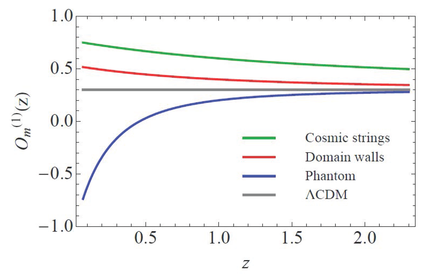
Once we consider a Hubble rate sample, it is possible to estimate confidence values of . If the test does not give a constant behaviour, then the ΛCDM model is ruled out and the existence of DE models or a curved ΛCDM scenario are considered. In the first option, several DE candidates can be related to (see Figure 1) by considering a specific value for , e.g., non-interacting cosmic strings with [47], static domain walls with [48,49] and phantom models with [13,14,15,16,17,18,19]. To distinguish between these models, we require the introduction of the diagnostic at the first-order in h, which is related to the dynamical test.
4. The Dynamical Om Diagnostic
A more meticulous analysis based on the abovementioned features takes into account a curved model, where the first derivatives of come on to the scene. Expressions for this case can be obtained by considering and in Equation (1):
from where we can find two expressions:
where the upper index ‘(2)’ indicates the existence of a second derivative of the luminosity distance. The calculations are explained in Appendix A.
To perform the distinctions between DE models, we can rewrite Equation (11) using Equation (10) and its derivative, which gives and , implying a ΛCDM model.
5. Observations of the Hubble Rate
To perform the diagnostic analysis, we require having at hand the observed data. This parameter has become an effective probe in cosmology comparison with SNIa, BAO and CMB data. In fact, it is more rewarding to study the observational data directly due to the fact that all these tests use the distance scale (e.g., the luminosity distance , the shift parameter R, or the distance parameter A) measurement to determine the values of the cosmological parameters, which needs the integral of and therefore loses some important information of this quantity.
depends on the differential age as a function of redshift z in the form: , which gives a direct measurement of through the change of redshift in cosmic time. As an independent approach of this measure, we provide two samples:
- (1)
- Cosmic Chronometers (C-C) data. This kind of sample gives a measurement of the expansion rate without relying on the nature of the metric between the chronometer and us. We are going to employ several data sets presented in [28]. A full compilation of the latter, which includes 28 measurements of in the range , are reported in [50]. The normalized parameter can be easily determined by considering the value km s−1 M pc−1 [46].
- (2)
- Data from BAO. Unlike the angular diameter measures given by the transverse BAO scale, the data can be extracted from the measurements of the line-of-sight of this BAO scale. Because the BAO distance scale is embodied in the CMB, its measurements on DE parameters are strongest at low redshift. The samples that we are going to consider consist of three data points from [34] and three more from [35] measured at six redshifts in the range . This data set is shown in Table 2.
6. Nonparametric Reconstructions
Following the same methodology proposed in [38], we are going to reconstruct the normalized Hubble parameter h using the Loess–Simex factory.
6.1. Reconstruction of
Step A1. Windows and subsample selection. We are going to select the proportion of observations fitting in a specific window. Each selection consists of some percentage of the total number of observations and to each subsample will be assigned a specific weighted least square local polynomial fit. We use a subsample via one quantity that is usually known in the statistical jargon as the smoothing parameter or span s, and we use , where k is the number of observations per window and rounded to the next largest integer, n is the total number of observations and s typically takes values that oscillate between 0 and 1. The election of the optimal value of s can be done by using cross-validation [51], which basically consists of omitting the ith observation from the local regression at the focal value . The cross-validation function is given by the expression
where is for span s. Using Equation (15), we calculated the values: for the C-C sample, for the BAO sample and for the C-C+BAO total sample, which correspond to 90, 85 and 40 percent of the data in each window, respectively. A detailed process can be found in [38].
Step A2. Weighted subsamples. Having already selected the amount of data in each window, consider a certain amount of data points near which are more related between them than others that are significantly far away and receive a null weight. This idea is encoded in the weight function described by a tricube kernel:
where , indicates the distance between the predictor redshift value for the i-th observation and the focal redshift . d is the maximum distance between the point of interest and elements inside the window.
Step A3. Regression analysis. Following the Loess technique, we consider a low-degree polynomial to perform a local fit of the subsample in each window:
A similar fit routine proposal was presented in [42]. The right hand side second term is related to , parameter that we will reconstruct in Section 6.2. As we can see from Equation (17), we shall consider a linear polynomial appropriate to fit each subset of data. Higher-degree polynomials are possible, and would work in theory, but it would result in models that are not really compliant with the spirit of Loess, which looks for a low-order polynomial and a simple model that can fit data easily. The reconstructed quantity is a weighted sum of the observations represented as:
where the weights in this regression are and .
Step A4. Simulated data sample. Simex is a simple simulation algorithm that allows for displaying the effect of measurement errors on parameter estimates. It consists of adding to the data sets an additional measurement error as follows:
where denotes the simulated data points and is the measurement error variance of each observation. The resulting measurement error is , in which we can extrapolate the data sample to an error free zone if . This zone is achieved after performing a standard regression, using a quadratic polynomial, of the data set computed for different values of λ. Specifically, we are going to consider as a starting value until increasing in steps of 0.1.
Step A5. Starting the reconstruction. After performing the latter extrapolation step, the data set will be simplified to the same length of the initial data, and, finally, these simulated data sets are normalized by , given as a result the reconstruction of . All of the above steps are repeated for all the data points in the astrophysical sample. The connection of the Loess–Simex reconstructed data points are represented by a curve due to the lack of parameter estimates. The reconstructed normalized Hubble parameter gives a general trend of the model.
Step A6. About the confidence regions. To design the confidence regions of the reconstructed parameter , we require the transfer uncertainties via error propagation given by
With this expression, we can calculate the uncertainties for the diagnostic
For the dynamical diagnostic, we have the following uncertainties:
As the set implies, we need to find the value of the variable . Let us start with the fitted value obtained in the Step A3. For nonparametric regression models, we estimate the error variance as
where is the residual for the i-th observation and is the equivalent degrees of freedom for the model, which, in our case, is equal to two. With this, we are capable of computing the variance of the fitted value at as:
The results of the latter are considered to compute the propagation values in Equation (20). Finally, the 68% confidence interval and the 95% confidence interval are given by and , respectively, and .
6.2. Reconstruction of
The logistics in this issue remains in the steps explained above. Nonetheless, we are going to proceed with a data set that only includes the coefficients related to the first derivative of .
Step B1. Reconstruction of . Let us proceed as in Step A1 until Step A3, where in the latter we performed a linear fit for these points using Equation (17). The fitting coefficients of our interest are determined by the evaluation of the polynomial in as , where the prime denotes differentiation with respect to z. The new data set will consist of these coefficients for the 28 simulated data points, to which we apply a least squares fit and then extrapolate to , giving us the data set that we normalize to obtain the values of and its respective curve as in Step A5.
Step B2. About the error propagation. Estimating the errors of and constructing a similar step as was developed with Equations (24) and (25) can be a little tricky, and it is necessary to be careful in the following methodology. This can be seen from the form of Equation (19), an expression that can be used similarly for if we have at hand the values of (already obtained in the linear fit performance in Step B1). The next question is: how we can compute the uncertainties of ? We need to start from Step A4, where we perform a least squares fit and the polynomial that we need to propagate now is
where the σ-values are the diagonal elements of the covariance matrix obtained from data set.
With the new set , we are ready to reproduce the same steps starting in Equation (19) and computing its error and matrix variance Equations (24) and (25). Until now, we have not taken yet into account any normalization of , an aspect that is implicit in the following propagation of errors
Finally, using this error propagation and its respective value, we can construct the confidence regions as in Step A6.
6.3. Nonparametric Reconstruction of the Diagnostic
On one hand, regarding the diagnostic for ΛCDM flat model (8), it is straightforward to compute the data set using the Loess–Simex estimate values calculated in Section 6. The values of are given directly from the new data set .
On the other hand, the uncertainty calculations are easily performed via Equation (21). Thereupon, we constructed the 68% and the 95% confidence intervals using the expressions: and , respectively.
As we discussed, the existence of a non-flat universe brings to the scene and . In this case, the system is given by Equations (13) and (14), which are independent of the values of the cosmological parameters and and imply a model that only relies on the values of our reconstructed and .
The confidence regions will be computed using the error propagation Equations (21) and (22) and the expressions: , and , .
7. Discussion and Conclusions
We developed the Loess–Simex factory to achieve two interesting goals. First, we performed the reconstruction of the normalized Hubble parameter , results that are represented by red dots (red line) in Figure 2, Figure 3 and Figure 4. In addition, in the upper plots of Figure 2, we illustrated the original data set represented by blue dots with its respective error values and its nonparametric reconstruction (red dots/line). It is interesting to note the comparison between these reconstructed points and the ΛCDM model, which is represented by a dotted green line.
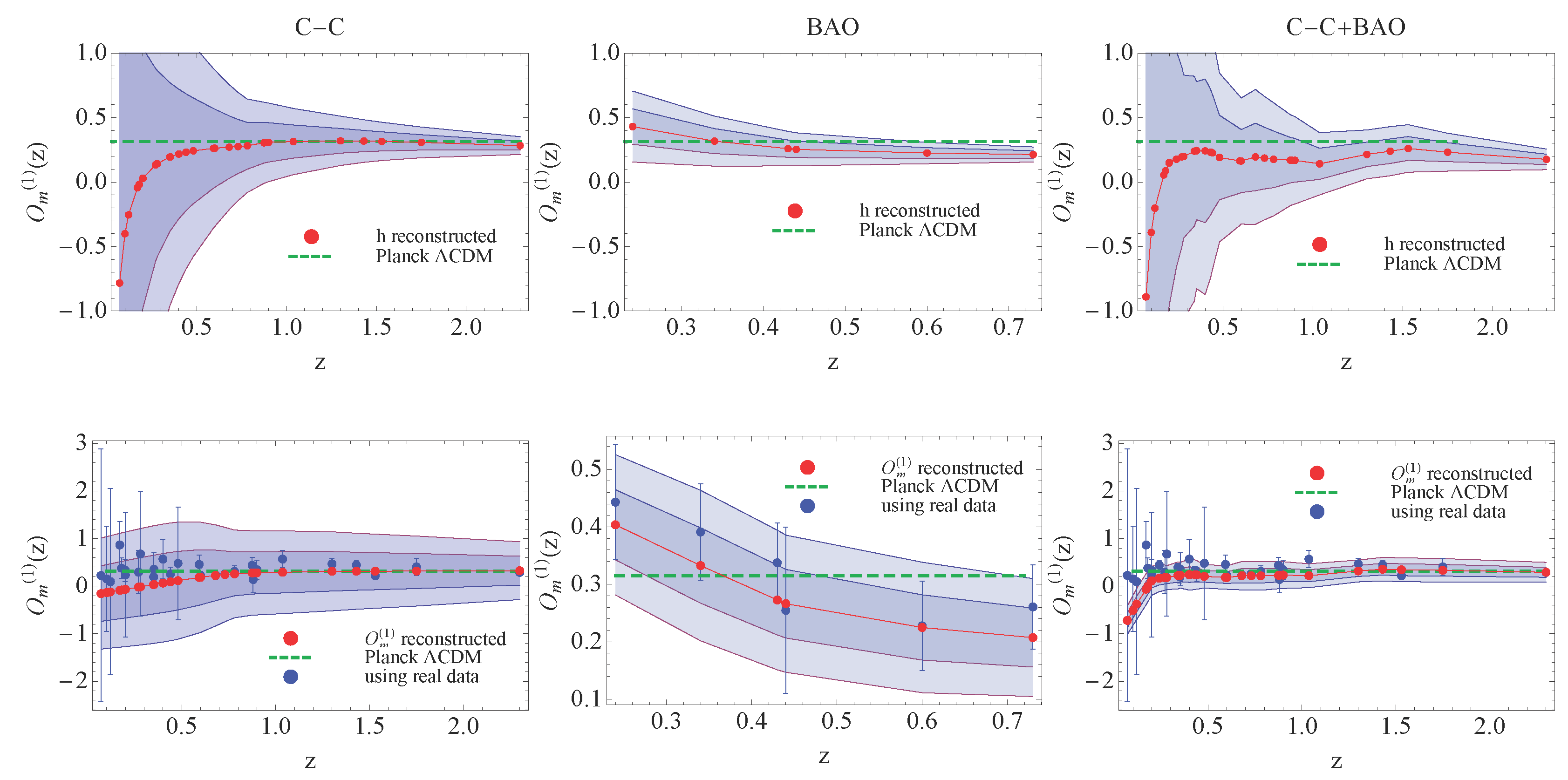
Our second goal was the reconstruction of the diagnostic and the and parameters using two astrophysical samples (C-C and BAO) for and the combination of them. The reconstruction of the diagnostic was made by considering two options: (I) using the already reconstructed h values (top of Figure 3) and (II) performing directly its reconstruction (bottom of Figure 3).
Let us discuss the results for each case.
For the C-C sample, the nonparametric reconstruction has the same trend as the one reported in [38]. However, in our case, we worked with the normalized Hubble parameter h, the behaviour of which is analogous to the previous case, as it is expected. The direct reconstruction of the diagnostic appears to be in good agreement with ΛCDM at . It is interesting to notice that, in this case, the confidence regions look smaller than in the case when we use the reconstructed h data.
For the BAO sample, unlike other proposals mentioned above, our results show a ΛCDM model that lies in our confidence contour reconstructions at 2-σ, even by performing the reconstruction with a few values of this data set. As in the previous sample, the direct reconstruction of this diagnostic gave a concordance model between 1 up to 2-σ. The reconstructions of and imply the reconstruction of , and the analysis shows large uncertainties. Even so, the reconstructions at high redshifts show a trend that possibly can loiter to ΛCDM at (see Figure 4, middle row).
For the C-C+BAO sample, we observe that the reconstruction is almost similar to the C-C case, clearly due to the amount of data of the first sample in comparison to the second sample. The concentration of data points at is related to the effects of the evaluation of the reconstructed data in Equation (8). We observed in the analysis a pull of the reconstructed curve up at , which probably shows the important relationship between derivatives of the data and the model itself. The direct reconstruction at zero-order loiters to ΛCDM up to , but because this is not a constant in the entire redshift range, we need to consider a dynamical test.
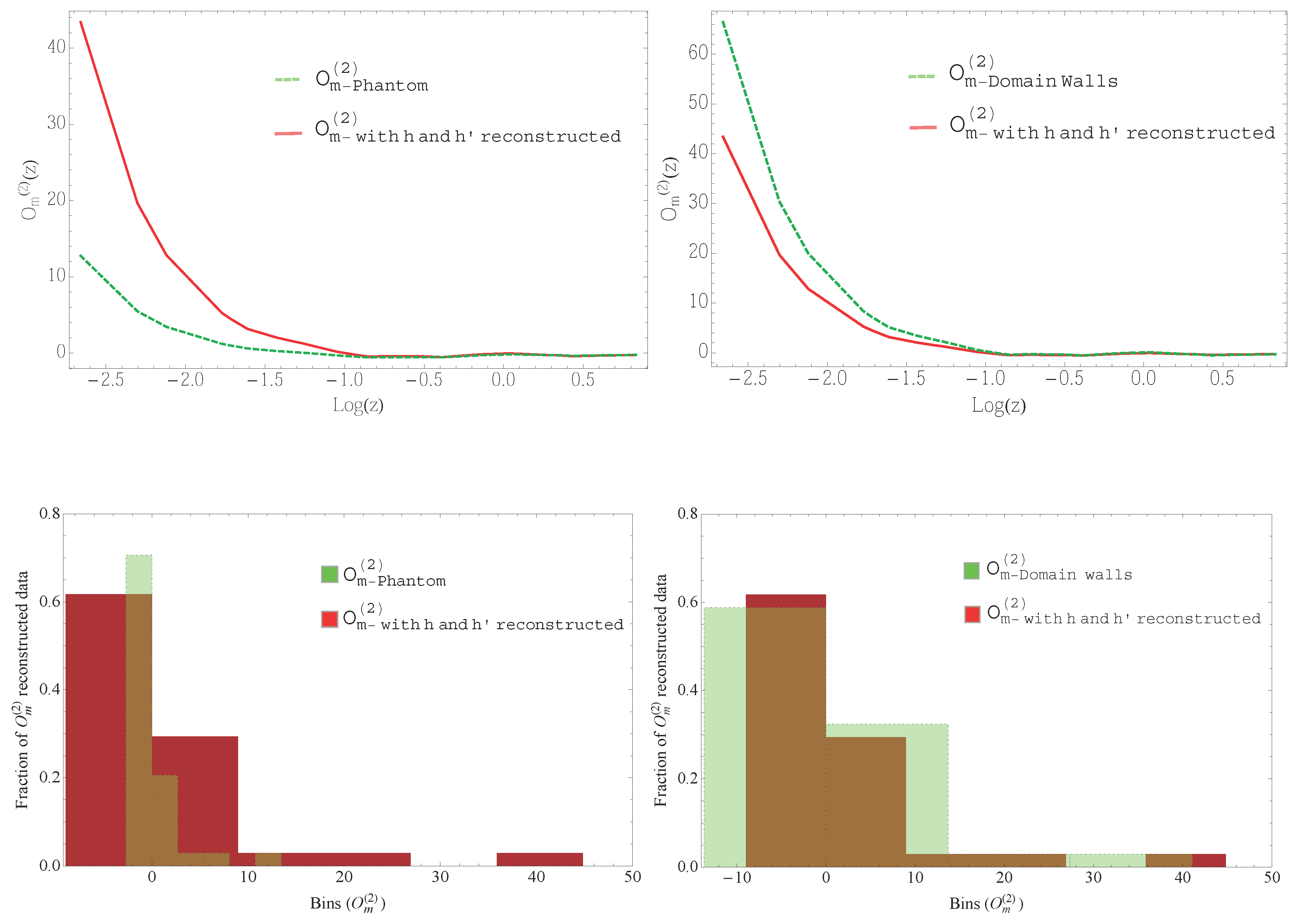
In order to find the adequate DE model in agreement with the reconstructions, we have performed a diagnostic (first-order in h, i.e., ), determining that even when the diagnostic hints to a phantom behaviour, when we enter in the region , the reconstructions have a preference for a EoS with known physical meaning , which corresponds to a static domain wall network in the entire redshift range. This EoS value is also able to reproduce the current cosmic acceleration in unified dark energy models [52,53,54,55,56,57]. At the top of Figure 5, we compare the dynamical diagnostics reconstructed (red curves) with diagnostics Equation (11) (green dashed curves) using two specific DE EoS models. How much is the fraction of the reconstructed data that make one DE model better than the other? To answer this, we calculated the probability of this fraction for each DE model in terms of the bins. The results are represented by the histograms at the bottom of Figure 5. The green bars represent DE models (phantom and static domain walls) and the red bars represent the amount of the reconstructed data. The bin widths for the reconstructed values are calculated by using [58]. We have that 62% of the reconstructed data lie in . Then, in this range, we observe that the amount of deviation between this data and each DE model corresponds to 8% for a phantom model and 3% for a static domain wall, making the latter a better model in agreement with the reconstructed data.
In addition, we notice the existence of poles in both analyses (see, for instance, Equations (8), (11) and (12)) only for the case when , which can be related with the problem of the phantom divide line. However, at least at this point in the diagnostic, this kind of divergence is an intrinsic problem that is not relevant since the current data available do not include . Forthcoming studies along the lines of these analyses promise to greatly improve with the use of high quality observations to make this nonparametric diagnostic more accurate and a very useful tool for testing alternative DE parameterizations and modify gravity proposals.
Acknowledgments
Celia Escamilla-Rivera is supported by the CNPq Fellowship and would like to thank Ruth Lazkoz for her opinions about the first ideas. Júlio C. Fabris would like to FAPES and CNPq (Brazil) for financial support. Both authors thank Winfried Zimdahl for his opinion on the final manuscript.
Author Contributions
Celia Escamilla-Rivera contributed with the new numerical analysis and code and as well with the statistical process behind the results. Júlio C. Fabris contributed to the analysis of the results.
Conflicts of Interest
The authors declare no conflict of interest.
Appendix A. Reconstruction of D(z)
In order to formulate a test for DE models, let us consider the derivative of the luminosity distance (5) and the distance-redshift (4) to obtain the following expressions:
from where we can extract the following cases:
- If we have a flat universe (), then the equations are
- For the case of a non-flat universe (), we have
From Equation (1), we can obtain an expression for the derivative of the distance-redshift
where is given by Equation (2), which is if and for a constant EoS. Possible scenarios are:
- For and ,
- For and ,
- For and ,
- For and ,
From Equation (A7), we obtain the first generalized equation for the diagnostic described by Equation (7).
When we consider a non-flat universe, the arises, and we are going to need a system of two equations: the first one given by Equation (10) and the second is the EoS when we rearranged Equation (3). After straightforward calculations and redefining and , we obtain the generalized equations for a non-flat universe and a constant dark energy EoS described by Equations (11) and (12).
References
- Laureijs, R.; Amiaux, J.; Arduini, S.; Auguères, J.-L.; Brinchmann, J.; Cole, R.; Cropper, M.; Dabin, C.; Duvet, L.; Ealet, A.; et al. Euclid Definition Study Report. arXiv 2011. [Google Scholar]
- Amendola, L.; Appleby, S.; Bacon, D.; Baker, T.; Baldi, M.; Bartolo, N.; Blanchard, A.; Bonvin, C.; Borgani, S.; Branchini, E.; et al. Cosmology and fundamental physics with the Euclid satellite. Living Rev. Relativ. 2013, 16, 6. [Google Scholar] [CrossRef]
- Samushia, L.; Reid, B.A.; White, M.; Percival, W.J.; Cuesta, A.J.; Zhao, G.; Ross, A.J.; Manera, M.; Aubourg, É.; Beutler, F.; et al. The Clustering of Galaxies in the SDSS-III Baryon Oscillation Spectroscopic Survey (BOSS): Measuring growth rate and geometry with anisotropic clustering. Mon. Not. R. Astron. Soc. 2014, 439, 3504–3519. [Google Scholar] [CrossRef]
- Abdalla, F.; Annis, J.; Bacon, D.; Bridle, S.; Castander, F.; Colless, M.; DePoy, D.; Diehl, H.T.; Eriksen, M.; Flaugher, B.; et al. The Dark Energy Spectrometer (DESpec): A Multi-Fiber Spectroscopic Upgrade of the Dark Energy Camera and Survey for the Blanco Telescope; Fermi National Accelerator Laboratory (FNAL): Batavia, IL, USA, 2012.
- Myers, S.T.; Abdalla, F.B.; Blake, C.; Koopmans, L.; Lazio, J.; Rawling, S. The Billion Galaxy Cosmological HI Large Deep Survey. In Astro2010: The Astronomy and Astrophysics Decadal Survey; The National Research Council of the National Academy of Sciences: Washington, DC, USA, 2009. [Google Scholar]
- Riess, A.G.; Filippenko, A.V.; Challis, P.; Clocchiattia, A.; Diercks, A.; Garnavich, P.M.; Gilliland, R.L.; Hogan, C.J.; Jha, S.; Kirshner, R.P.; et al. Observational Evidence from Supernovae for an Accelerating Universe and a Cosmological Constant. Astron. J. 1998, 116, 1009–1038. [Google Scholar] [CrossRef]
- Perlmutter, S.; Aldering, G.; Goldhaber, G.; Knop, R.A.; Nugent, P.; Castro, P.G.; Deustua, S.; Fabbro, S.; Goobar, A.; Groom, D.E.; et al. Measurements of Omega and Lambda from 42 High-Redshift Supernovae. Astrophys. J. 1999, 517, 565–586. [Google Scholar] [CrossRef]
- Eisenstein, D.J.; Zehavi, I.; Hogg, D.W.; Scoccimarro, R.; Blanton, M.R.; Nichol, R.C.; Scranton, R.; Seo, H.; Tegmark, M.; Zheng, Z.; et al. Detection of the Baryon Acoustic Peak in the Large-Scale Correlation Function of SDSS Luminous Red Galaxies. Astrophys. J. 2005, 633, 560–574. [Google Scholar] [CrossRef]
- Spergel, D.N.; Verde, L.; Peiris, H.V.; Komatsu, E.; Nolta, M.R.; Bennett, C.L.; Halpern, M.; Hinshaw, G.; Jarosik, N.; Kogut, A.; et al. First Year Wilkinson Microwave Anisotropy Probe (WMAP) Observations: Determination of Cosmological Parameters. Astrophys. J. Suppl. 2003, 148, 175–194. [Google Scholar] [CrossRef]
- Tegmark, M.; Strauss, M.; Blanton, M.; Abazajian, K.; Dodelson, S.; Sandvik, H.; Wang, X.; Weinberg, D.; Zehavi, I.; Bahcall, N.; et al. Cosmological parameters from SDSS and WMAP. Phys. Rev. D 2004, 69, 103501. [Google Scholar] [CrossRef]
- Jain, B.; Taylor, A. Cross-correlation Tomography: Measuring Dark Energy Evolution with Weak Lensing. Phys. Rev. Lett. 2003, 91, 141302. [Google Scholar] [CrossRef] [PubMed]
- Perivolaropoulos, L. LCDM: Triumphs, Puzzles and Remedies. J. Cosmol. 2011, 15, 6054–6064. [Google Scholar]
- Gong, Y.; Zhang, Y.Z. Probing the curvature and dark energy. Phys. Rev. D 2005, 72, 043518. [Google Scholar] [CrossRef]
- Jassal, H.K.; Bagla, J.S.; Padmanabhan, T. WMAP constraints on low redshift evolution of dark energy. Month. Not. R. Astron. Soc. 2005, 356, L11–L16. [Google Scholar] [CrossRef]
- Padmanabhan, T.; Choudhury, T.R. A theoretician’s analysis of the supernova data and the limitations in determining the nature of dark energy. Month. Not. R. Astron. Soc. 2003, 344, 823–834. [Google Scholar]
- Huterer, D.; Turner, M.S. Probing dark energy: Methods and strategies. Phys. Rev. D 2001, 64, 123527. [Google Scholar] [CrossRef]
- Choudhury, T.R.; Padmanabhan, T. Cosmological parameters from supernova observations: A critical comparison of three data sets. Astron. Astrophys. 2005, 429, 807–818. [Google Scholar] [CrossRef]
- Wetterich, C. Phenomenological parameterization of quintessence. Phys. Lett. B 2004, 594, 17–22. [Google Scholar] [CrossRef]
- Upadhye, A.; Ishak, M.; Steinhardt, P.J. Dynamical dark energy: Current constraints and forecasts. Phys. Rev. D 2005, 72, 063501. [Google Scholar] [CrossRef]
- Lee, S. Constraints on the dark energy equation of state from the separation of CMB peaks and the evolution of alpha. Phys. Rev. D 2005, 72, 123528. [Google Scholar] [CrossRef]
- Barai, P.; Das, T.K.; Wiita, P.J. The dependence of general relativistic accretion on black hole spin. Astrophys. J. 2004, 613, L49–L52. [Google Scholar] [CrossRef]
- Linder, E.V. Paths of quintessence. Phys. Rev. D 2006, 73, 063010. [Google Scholar] [CrossRef]
- Lazkoz, R.; Salzano, V.; Sendra, I. Oscillations in the dark energy equation of state: New MCMC lessons. Phys. Lett. B 2010, 694, 198–208. [Google Scholar] [CrossRef]
- Ma, J.-Z.; Zhang, X. Probing the dynamics of dark energy with novel parametrizations. Phys. Lett. B 2011, 699, 233–238. [Google Scholar] [CrossRef]
- Sahni, V.; Shafieloo, A.; Starobinsky, A.A. Two new diagnostics of dark energy. Phys. Rev. D 2008, 78, 103502. [Google Scholar] [CrossRef]
- Shafieloo, A.; Sahni, V.; Starobinsky, A.A. A new null diagnostic customized for reconstructing the properties of dark energy from BAO data. Phys. Rev. D 2012, 86, 103527. [Google Scholar] [CrossRef]
- Seikel, M.; Yahya, S.; Maartens, R.; Clarkson, C. Using H(z) data as a probe of the concordance model. Phys. Rev. D 2012, 86, 083001. [Google Scholar] [CrossRef]
- Simon, J.; Verde, L.; Jimenez, R. Constraints on the redshift dependence of the dark energy potential. Phys. Rev. D 2005, 71, 123001. [Google Scholar] [CrossRef]
- Stern, D.; Jimenez, R.; Verde, L.; Kamionkowski, M.; Stanford, S.A. Cosmic Chronometers: Constraining the Equation of State of Dark Energy. I: H(z) Measurements. J. Cosmol. Astropart. Phys. 2010. [Google Scholar] [CrossRef]
- Zhang, C.; Zhang, H.; Yuan, S.; Zhang, T.J.; Sun, Y.C. Four New Observational H(z) Data From Luminous Red Galaxies of Sloan Digital Sky Survey Data Release Seven. Res. Astron. Astrophys. 2014, 14, 1221–1233. [Google Scholar] [CrossRef]
- Blake, C.; Glazebrook, K.; Davis, T.; Brough, S.; Colless, M.; Contreras, C.; Couch, W.; Croom, S.; Drinkwater, M.J.; Forster, K.; et al. The WiggleZ Dark Energy Survey: Measuring the cosmic expansion history using the Alcock-Paczynski test and distant supernovae. Mon. Not. R. Astron. Soc. 2011, 418, 1725–1735. [Google Scholar] [CrossRef]
- Chuang, C.H.; Wang, Y. Modeling the Anisotropic Two-Point Galaxy Correlation Function on Small Scales and Improved Measurements of H(z), DA(z), and f(z)sigma8(z) from the Sloan Digital Sky Survey DR7 Luminous Red Galaxies. Mon. Not. R. Astron. Soc. 2013, 435, 255–262. [Google Scholar] [CrossRef]
- Moresco, M.; Cimatti, A.; Jimenez, R.; Pozzetti, L.; Zamorani, G.; Bolzonella, M.; Dunlop, J.; Lamareille, F.; Mignoli, M.; Pearce, H.; et al. Improved constraints on the expansion rate of the Universe up to z 1.1 from the spectroscopic evolution of cosmic chronometers. J. Cosmol. Astropart. Phys. 2012. [Google Scholar] [CrossRef] [PubMed]
- Blake, C.; Brough, S.; Colless, M.; Contreras, C.; Couch, W.; Croom, S.; Croton, D.; Davis, T.; Drinkwater, M.J.; Forster, K.; et al. The WiggleZ Dark Energy Survey: Joint measurements of the expansion and growth history at z < 1. Mon. Not. R. Astron. Soc. 2012, 425, 405–414. [Google Scholar]
- Gaztanaga, E.; Cabre, A.; Hui, L. Clustering of Luminous Red Galaxies IV: Baryon Acoustic Peak in the Line-of-Sight Direction and a Direct Measurement of H(z). Mon. Not. R. Astron. Soc. 2009, 399, 1663–1680. [Google Scholar] [CrossRef]
- Holsclaw, T.; Alam, U.; Sanso, B.; Lee, H.; Heitmann, K.; Habib, S.; Higdon, D. Nonparametric Dark Energy Reconstruction from Supernova Data. Phys. Rev. Lett. 2010, 105, 241302. [Google Scholar] [CrossRef] [PubMed]
- Shafieloo, A.; Kim, A.G.; Linder, E.V. Gaussian Process Cosmography. Phys. Rev. D 2012, 85, 123530. [Google Scholar] [CrossRef]
- Montiel, A.; Lazkoz, R.; Sendra, I.; Escamilla-Rivera, C.; Salzano, V. Nonparametric reconstruction of the cosmic expansion with local regression smoothing and simulation extrapolation. Phys. Rev. D 2014, 89, 043007. [Google Scholar] [CrossRef]
- Cleveland, W.S. Robust Locally Weighted Regression and Smoothing Scatterplots. J. Am. Stat. Assoc. 1979, 74, 829–836. [Google Scholar] [CrossRef]
- Apanasovich, T.; Carroll, J.; Maity, A. SIMEX and standard error estimation in semiparametric measurement error models. Electron. J. Stat. 2009, 3, 318–348. [Google Scholar] [CrossRef] [PubMed]
- Press, W.H.; Teukolsky, S.A.; Vetterling, W.T.; Flannery, B.P. Numerical Recipes, 3rd ed.; Cambridge Press: Cambridge, UK, 1992. [Google Scholar]
- Daly, R.A.; Djorgovski, S.G. A Model-Independent Determination of the Expansion and Acceleration Rates of the Universe as a Function of Redshift and Constraints on Dark Energy. Astrophys. J. 2003, 597, 9–20. [Google Scholar] [CrossRef]
- Capozziello, S.; de Laurentis, M.; Luongo, O.; Ruggeri, A. Cosmographic Constraints and Cosmic Fluids. Galaxies 2013, 1, 216–260. [Google Scholar] [CrossRef]
- Dunsby, P.K.S.; Luongo, O. On the theory and applications of modern cosmography. Int. J. Geom. Meth. Mod. Phys. 2016, 13, 1630002. [Google Scholar] [CrossRef]
- Lazkoz, R.; Alcaniz, J.; Escamilla-Rivera, C.; Salzano, V.; Sendra, I. BAO cosmography. J. Cosmol. Astropart. Phys. 2013, 12, 5. [Google Scholar] [CrossRef] [PubMed]
- Ade, P.A.R.; Aghanim, N.; Arnaud, M.; Ashdown, M.; Aumont, J.; Baccigalupi, C.; Banday, A.J.; Barreiro, R.B.; Bartlett, J.G.; Bartolo, N.; et al. Planck 2015 results. XIII. Cosmological parameters. Astron. Astrophys. 2015, 594, A13. [Google Scholar]
- Alam, U.; Sahni, V.; Saini, T.D.; Starobinsky, A.A. Exploring the Expanding Universe and Dark Energy using the Statefinder Diagnostic. Mon. Not. R. Astron. Soc. 2003, 344, 1057–1074. [Google Scholar] [CrossRef]
- Friedland, A.; Murayama, H.; Perelstein, M. Domain Walls as Dark Energy. Phys. Rev. D 2003, 67, 043519. [Google Scholar] [CrossRef]
- Pina Avelino, P.; Martins, C.J.A.P.; Menezes, J.; Menezes, R.; Oliveira, J.C.R.E. Frustrated Expectations: Defect Networks and Dark Energy. Phys. Rev. D 2006, 73, 123519. [Google Scholar] [CrossRef]
- Farooq, O.; Ratra, B. Hubble parameter measurement constraints on the cosmological deceleration-acceleration transition redshift. Astrophys. J. Lett. 2013, 766, L7. [Google Scholar] [CrossRef]
- Fox, J. Applied Regression Analysis and Generalized Linear Models, 2nd ed.; SAGE Publications: New York, NY, USA, 2008. [Google Scholar]
- Gonzalez-Diaz, P.F. Unified Model for Dark Energy. Phys. Lett. B 2003, 562, 1–8. [Google Scholar] [CrossRef]
- Bento, M.C.; Bertolami, O.; Sen, A.A. The Revival of the Unified Dark Energy-Dark Matter Model? Phys. Rev. D 2004, 70, 083519. [Google Scholar] [CrossRef]
- Park, C.G.; Hwang, J.C.; Park, J.; Noh, H. Observational constraints on a unified dark matter and dark energy model based on generalized Chaplygin gas. Phys. Rev. D 2010, 81, 063532. [Google Scholar] [CrossRef]
- De-Santiago, J.; Cervantes-Cota, J.L. Generalizing a Unified Model of Dark Matter, Dark Energy, and Inflation with Non Canonical Kinetic Term. Phys. Rev. D 2011, 83, 063502. [Google Scholar] [CrossRef]
- Xu, L.; Wang, Y.; Noh, H. Constraints to Holographic Dark Energy Model via Type Ia Supernovae, Baryon Acoustic Oscillation and WMAP. Phys. Rev. D 2012, 85, 043003. [Google Scholar]
- Luongo, O.; Quevedo, H. A unified dark energy model from a vanishing speed of sound with emergent cosmological constant. Int. J. Mod. Phys. D 2014, 23, 1450012. [Google Scholar]
- Scott, D.W. Scott’s rule. WIREs Comput. Stat. 2010, 2, 497–502. [Google Scholar]
Figure 1.
Comparison between dark energy models. The solid grey line represents a ΛCDM model with . Non-interacting cosmic strings with are represented by the green line. Static domain walls with are represented by the red line, and the phantom model with is represented by the blue line.
Figure 1.
Comparison between dark energy models. The solid grey line represents a ΛCDM model with . Non-interacting cosmic strings with are represented by the green line. Static domain walls with are represented by the red line, and the phantom model with is represented by the blue line.

Figure 2.
Reconstruction of , and parameters for C-C data (left column), BAO data (middle column) and C-C+BAO data (right column). The red dots (line) are (is) the Loess–Simex results for each sample. The dashed green line is ΛCDM with . Shaded yellow areas represent the 68% and 95% confidence regions. Top row: Loess–Simex reconstructions. The blue dots are the real data sample with its respective error bars; Middle row: Loess–Simex reconstructions. The blue dots represent the normalized real data h with its respective error propagation bars; Bottom row: Loess–Simex reconstructions. The purple dots represent the values of the second coefficient after performing a Loess routine fit, which also gives the uncertainty bars via the covariance matrix.
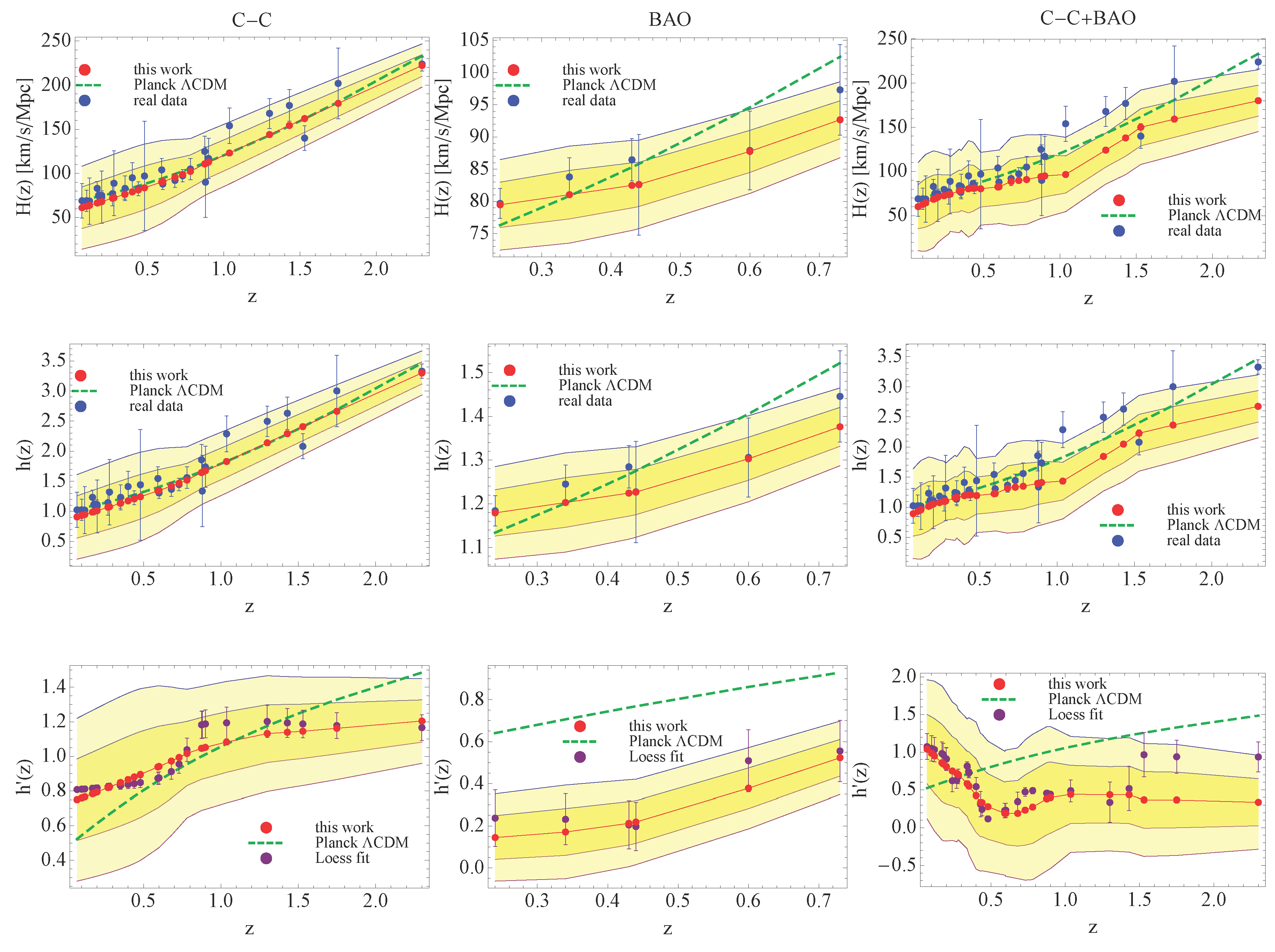
Figure 3.
Reconstruction of the diagnostic for C-C data (left column), BAO data (middle column) and C-C+BAO data (right column). The red dots (line) are (is) the Loess–Simex results for each sample. The dashed green line is . Shaded purple areas represent the 68% and 95% confidence regions. Top row: diagnostic with h reconstructed via Loess–Simex; Bottom row: values reconstructed directly via Loess–Simex. The blue dots are these values using h normalized with its error propagation bars.

Figure 4.
Reconstruction of the and diagnostics for C-C data (left column), BAO data (middle column) and C-C+BAO data (right column). The red dots (line) are (is) the reconstructed values using the reconstructed h and via Loess–Simex. The dashed green line is . Shaded purple areas represent the 68% and 95% confidence regions. Top row: diagnostic with h and reconstructed via Loess–Simex; Bottom row: diagnostic with h and reconstructed via Loess–Simex.
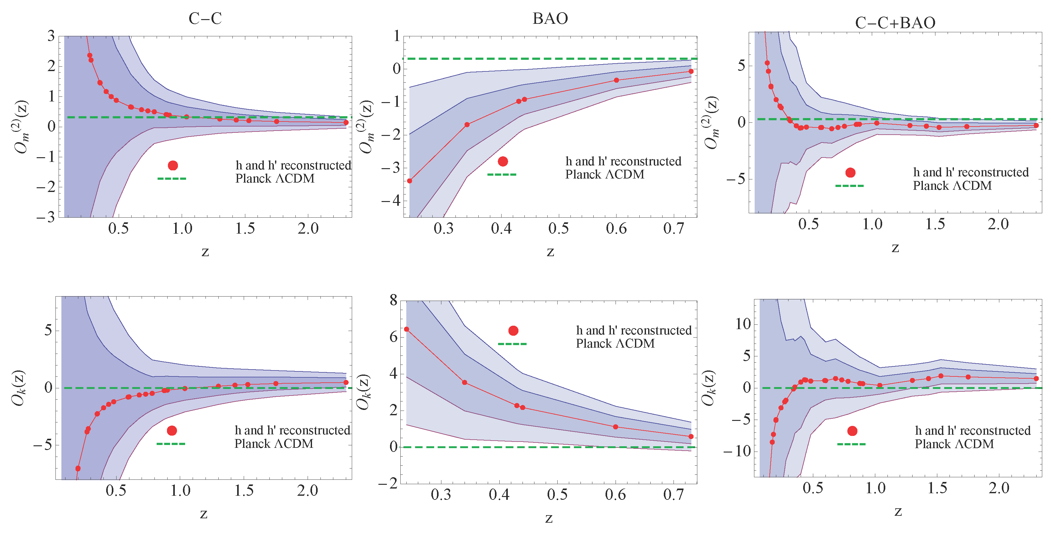
Figure 5.
Top: Comparison between DE models: phantom and static domain walls and the reconstructed using C-C+BAO data. The green dashed lines represent Equation (11) for a phantom () and static domain walls () models . The red solid lines represent the diagnostic using the reconstructed h and . We observe on the right-hand side plot that the static domain walls model appears to be more in agreement with the diagnostic reconstructed in comparison to the left plot where the phantom model starts to deviate from the reconstructed at low redshifts (); Bottom: Probability comparison between DE models. The green bars represent DE models (phantom and static domain walls) and the red bars represent the amount of the reconstructed data. In addition, a 62% fraction of the reconstructed data lies in , and then, in this range, we observe that the amount of deviation between this data and each DE model corresponds to 8% for a phantom model and 3% for a static domain wall. These probabilities support the results obtained above.

Table 1.
Features in the diagnostic with respect to the value of , which can be taken from recent Planck results [46] and a constant EoS .
| EoS | Om Diagnostic | Model |
|---|---|---|
| Flat ΛCDM. | ||
| Quintessence. | ||
| Phantom. |
© 2016 by the authors; licensee MDPI, Basel, Switzerland. This article is an open access article distributed under the terms and conditions of the Creative Commons Attribution (CC-BY) license (http://creativecommons.org/licenses/by/4.0/).
Share and Cite
MDPI and ACS Style
Escamilla-Rivera, C.; Fabris, J.C. Nonparametric Reconstruction of the Om Diagnostic to Test ΛCDM. Galaxies 2016, 4, 76. https://doi.org/10.3390/galaxies4040076
AMA Style
Escamilla-Rivera C, Fabris JC. Nonparametric Reconstruction of the Om Diagnostic to Test ΛCDM. Galaxies. 2016; 4(4):76. https://doi.org/10.3390/galaxies4040076
Chicago/Turabian StyleEscamilla-Rivera, Celia, and Júlio C. Fabris. 2016. "Nonparametric Reconstruction of the Om Diagnostic to Test ΛCDM" Galaxies 4, no. 4: 76. https://doi.org/10.3390/galaxies4040076
Note that from the first issue of 2016, this journal uses article numbers instead of page numbers. See further details here.