Exploring the Behaviour of Long Gamma-Ray Bursts with Intrinsic Afterglow Correlations: log L_200s−α_>200s

Abstract

In these proceedings, we summarise the exploration so far of the relationship between the afterglow luminosity (measured at rest frame 200s; $\log {\mathrm{L}}_{200\mathrm{s}}$) and average afterglow decay rate (measured from rest frame 200s onwards, ${\alpha }_{>200\mathrm{s}}$) of long duration Gamma-ray Bursts (GRBs), first reported in the optical/UV light curves of GRB afterglows. We show that this correlation is also present in the X-ray afterglows of GRBs as observed by Swift-XRT. We explore how the parameters of the correlation observed in both the X-ray and optical/UV light curves relate to each other and the prompt emission phase and whether these correlations are consistent with predictions of the standard afterglow model. We find that the observed correlations are consistent with a common underlying physical mechanism producing GRBs and their afterglows regardless of the detailed temporal behaviour. However, a basic afterglow model has difficulty explaining all the observed correlations. This leads us to briefly discuss alternative more complex models.

1. Introduction

Statistical investigations of large samples of Gamma-ray bursts (GRBs) aim to find common characteristics and correlations that link individual events and therefore provide insight into the mechanisms common to GRBs. The luminosity distribution of GRB afterglow light curves is clustered and appears to be wider at early times and narrows as the afterglows fade. This points towards the brightest GRB afterglows decaying more quickly than the less luminous afterglows. In [1], we explored this hypothesis using a sample of optical/UV light curves. We tested for a correlation between logarithmic brightness (measured at rest frame 200s), $\log {\mathrm{L}}_{200\mathrm{s}}$ and average decay rate of GRB afterglows (measured from rest frame 200s onwards), ${\alpha }_{>200\mathrm{s}}$. A Spearman rank correlation gave a coefficient of −0.58 at a significance of 4.2σ ([1]). Thus confirming our observation that the brightest GRB afterglows, at least in the optical/UV, decay more quickly than the less luminous afterglows.

In this conference proceeding, we summarize work presented in [2,3] on the exploration of this luminosity–decay correlation. We first show that the luminosity–decay correlation is also observed in the X-rays. We discuss whether the correlation we observe in the X-rays is affected by the morphology of the light curves [4,5,6], which tends to be more complex than the optical/UV. We also explore how the optical/UV and X-ray correlation parameters relate to the prompt emission phase and determine whether our sample results in correlations consistent with those predicted by the standard afterglow model using a Monte Carlo simulation.

To test for the correlation in the X-rays, we collate luminosity light curves from all GRBs discovered by Swift-BAT with X-ray afterglows detected by Swift-XRT and measured redshifts, discovered between December 2004 and March 2014; further details on sample selection can be found in [2]. There are 280 GRBs in our sample that fit these criteria. When comparing the parameters from the optical/UV and X-ray light curves, we use the sample of 48 GRBs used by [3].

For each GRB, we interpolated the optical light curves between rest frame 100 and 2000s to obtain the optical luminosity at rest frame 200s and for the X-ray we measured the luminosity at rest frame 200s from the best fit light curve model. To obtain the average decay rate, we fit a single power-law to each optical and X-ray light curve using data from rest frame 200s onwards. To determine the degree of correlation and the relationship between these and other parameters, we use both Spearman rank correlation and linear regression. All uncertainties throughout these proceedings are quoted at 1σ. The flux density is expressed throughout this proceeding as $F(t,\nu )\propto t^{\alpha }{\nu }^{\beta }$, where α and β are the temporal and spectral indices respectively, except for Figure 1 and Figure 2, where we use the absolute values of these indices. Throughout, we assume the Hubble parameter $H_0=70{\mathrm{km}\mathrm{s}}^{-1}{\mathrm{Mpc}}^{-1}$ and density parameters ${\mathrm{\Omega }}_{\mathrm{\Lambda }}=0.7$ and ${\mathrm{\Omega }}_m=0.3$.

2. Results

2.1. X-Ray Afterglow $\mathrm{Log}{\mathrm{L}}_{200\mathrm{s}}-{\alpha }_{>200\mathrm{s}}$ Correlation

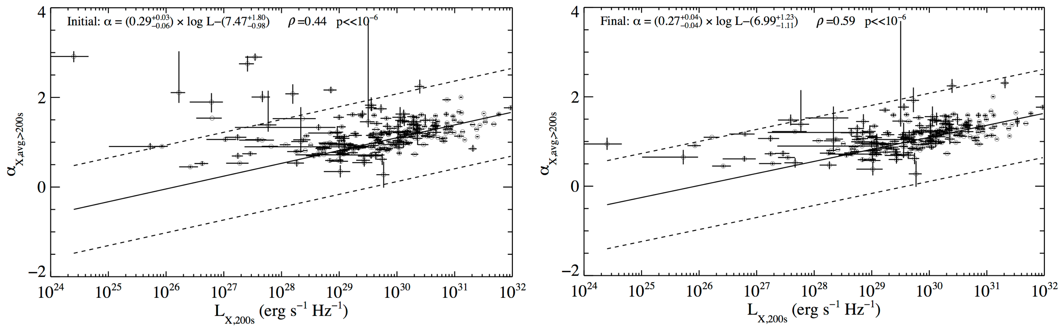
In the left hand panel of Figure 1, using the sample of 280 X-ray afterglows, we show evidence for a correlation between $\log {\mathrm{L}}_{\mathrm{X},200\mathrm{s}}-{\alpha }_{X,>200\mathrm{s}}$, although there is much scatter. Some of the scatter is likely due to the sample consisting of both long and short GRBs, some of the X-ray afterglows may be contaminated by a steep decay which affects both the luminosity and average decay index, and X-ray flares may be present which may also affect the average decay index. Steep decays and flares are likely produced by the prompt emission rather than the afterglow. For GRBs where the prompt emission contaminates the light curve, we re-computed the average decay index using only data beyond rest frame 200s that is not dominated by the steep decay and we also exclude flaring episodes. We also recomputed the luminosity at rest frame 200s to get a better estimate of the afterglow brightness at this time by extrapolating the decay index of the segment closest to rest frame 200s from the best fit afterglow model (see [2] for further details).

After correcting for steep decay contamination, flares and filtering on long duration GRBs the final correlation is presented in the right panel of Figure 1. Much of the scatter in the correlation has been reduced.

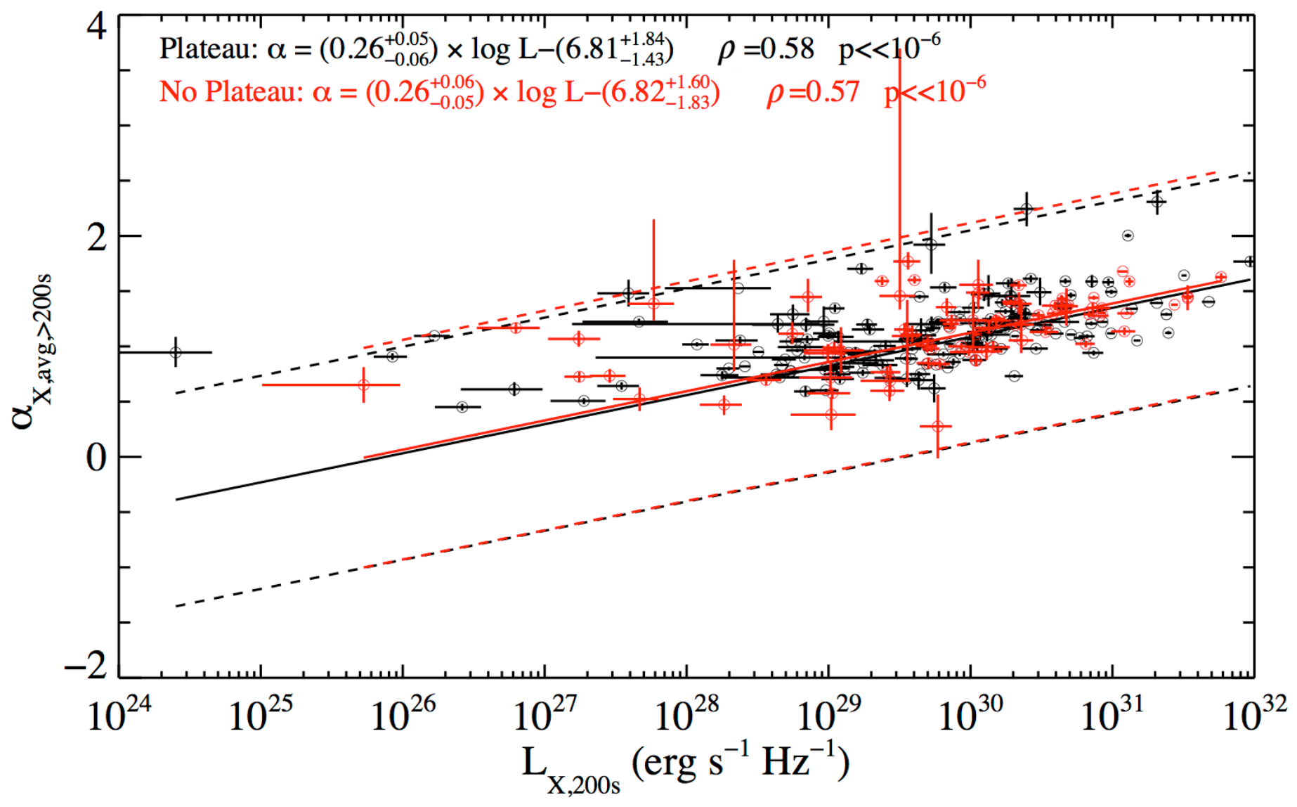
Since there is a correlation between the time and flux of the end of the X-ray plateau [7,8], which could be the dominating factor in the luminosity–decay correlation, we test the effect of X-ray plateaus by separating our sample into those light curves that show plateau behavior (defined as containing segment II in criteria set by [9]), and those that do not show clear plateaus. Figure 2 demonstrates that the average decay-luminosity correlation is significant in both the sample with and without plateaus. This suggests that the presence of a plateau is not necessarily solely responsible for regulating the average afterglow decay.

2.2. Comparison of Optical/UV, X-Ray and Prompt Emission

In

Table 1. For each pair of parameters examined, this table provides the Spearman rank correlation coefficient with its associated null hypothesis; the slope and constant values provided by the best fit linear regression. For comparison with our Monte Carlo simulations in Section 3, we also provide the $1\sigma$ error of the Spearman rank coefficient (Adapted from Table 2 in [3]).

Parameters		Spearman Rank	Null	—Best Fit Linear Regression—
$\mathit{x}$-axis	$\mathit{y}$-axis	Coefficient	Hypothesis	Slope	Constant
$\log {\mathrm{L}}_{\mathrm{O},200\mathrm{s}}$	$\log {\mathrm{L}}_{\mathrm{X},200\mathrm{s}}$	0.81 (0.05)	5.26 × 10−12	0.91 ± 0.22	1.04 ± 6.94
${\alpha }_{O,>200\mathrm{s}}$	${\alpha }_{X,>200\mathrm{s}}$	0.77 (0.07)	1.10 × 10−10	0.97 ± 0.10	−0.25 ± 0.09
$\log {\mathrm{L}}_{\mathrm{O},200\mathrm{s}}$	${\alpha }_{O,>200\mathrm{s}}$	−0.58 (0.11)	1.90 × 10−5	−0.28 ± 0.04	7.72 ± 1.31
$\log {\mathrm{L}}_{\mathrm{X},200\mathrm{s}}$	${\alpha }_{X,>200\mathrm{s}}$	−0.69 (0.09)	8.03 × 10−8	−0.26 ± 0.05	6.71 ± 1.39
$\log {\mathrm{L}}_{\mathrm{O},200\mathrm{s}}$	${\alpha }_{X,>200\mathrm{s}}$	−0.60 (0.12)	6.87 × 10−6	−0.29 ± 0.03	8.13 ± 1.08
$\log {\mathrm{L}}_{\mathrm{X},200\mathrm{s}}$	${\alpha }_{O,>200\mathrm{s}}$	−0.65 (0.10)	5.58 × 10−7	−0.32 ± 0.06	8.70 ± 1.68

, we show the results of correlations comparing the X-ray and optical/UV $\log {\mathrm{L}}_{200\mathrm{s}}-{\alpha }_{>200\mathrm{s}}$ correlation parameters for the reduced sample of 48 GRBs. There is a strong correlation between the luminosities of the two bands and also their average decay indices are strongly correlated. Also, we see that the $\log {\mathrm{L}}_{200\mathrm{s}}-{\alpha }_{>200\mathrm{s}}$ correlations are consistent within $1\sigma$. In Table 1, we also provide the relationships derived when swapping the X-ray and optical/UV luminosity decay parameters, i.e., $\log {\mathrm{L}}_{\mathrm{O},200\mathrm{s}}$ versus ${\alpha }_{X,>200\mathrm{s}}$ and $\log {\mathrm{L}}_{\mathrm{X},200\mathrm{s}}$ versus ${\alpha }_{O,>200\mathrm{s}}$. The fact that significant correlations are found even when mixing decay and luminosity parameters between the optical/UV and X-ray bands provides support to the luminosity–decay correlations.

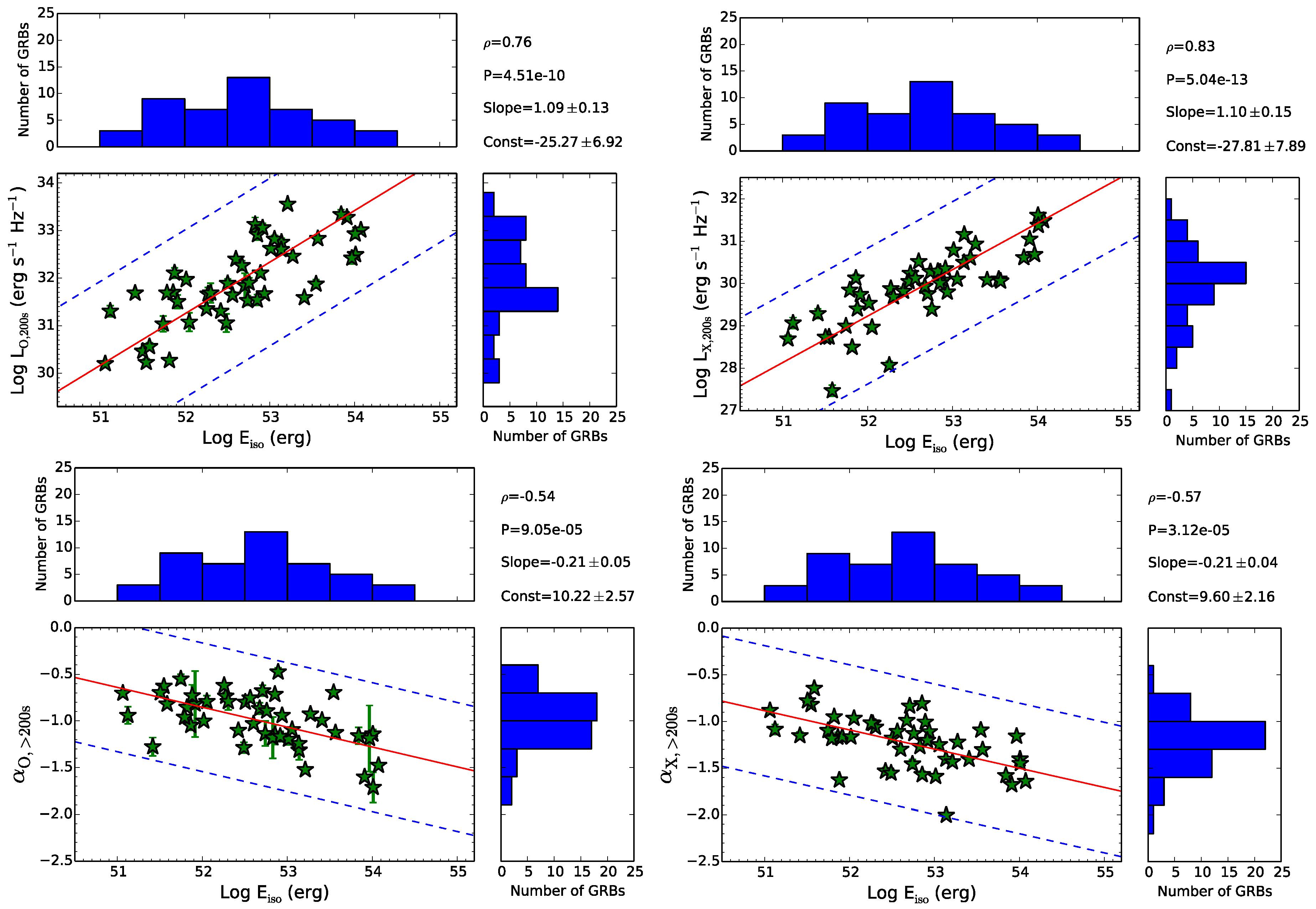
We also show in Figure 3 these parameters in comparison with the prompt emission parameter ${\mathrm{E}}_{\mathrm{iso}}$, isotropic energy. Correlations between afterglow luminosity and isotropic energy have been previously reported (e.g., [10,11,12]). For both the optical/UV and X-ray light curves, the linear regressions of the $\log {\mathrm{L}}_{200\mathrm{s}}$ and $\log {\mathrm{E}}_{\mathrm{iso}}$, give consistent results within $1\sigma$ errors. The bottom two panels of Figure 3 display $\log {\mathrm{E}}_{\mathrm{iso}}$ against ${\alpha }_{O,>200\mathrm{s}}$ and ${\alpha }_{X,>200\mathrm{s}}$. The linear regression for both the optical/UV and X-ray decay indices against $\log {\mathrm{E}}_{\mathrm{iso}}$ are consistent with each other and indicate correlations between the average decay indices and isotropic energy. This suggests that the more energetic the prompt emission, the faster the average decay of the X-ray and optical/UV afterglows.

3. Monte Carlo Simulation

The standard afterglow synchrotron model is currently the favoured scenario in terms of producing the observed X-ray-optical afterglow emission. In this model, the afterglow is a natural result of the collimated ejecta reaching the external medium and interacting with it, producing the observed synchrotron emission. The observed flux depends on the properties and environment of the GRB and there is usually more than one relationship to describe how two parameters are related (e.g., [13,14]). This therefore makes a simple analytic prediction of the expected relationships in a sample of observed parameters difficult to determine. We therefore use a Monte Carlo simulation to determine the expected relationships. We assume a basic isotropic, collimated outflow which is not energy injected and since we wish to consider a very simplistic model we do not consider the emission from the traditional reverse shock (e.g., [15]). We simulate the optical and X-ray $\log {\mathrm{L}}_{200\mathrm{s}}$ and ${\alpha }_{>200\mathrm{s}}$ for a sample of 48 GRBs, which we repeat ${10}^4$ times. To produce these values, we draw randomly on distributions of the fraction of energy given to the electrons, ${ϵ}_e$; the fraction of energy given to the magnetic field, ${ϵ}_B$; the density of the external medium (assuming constant density); the electron energy index, p; prompt emission energy, ${\mathrm{E}}_{\mathrm{iso}}$, efficiency η and redshift, z (see [3] for further details). For each simulated sample, we performed a linear regression and we also calculated the Spearman rank coefficient between several observable parameters. The predictions for the correlations are taken as the mean and the 1σ error from the distribution of results and are given in

Table 2. The Spearman rank coefficient and linear regression parameters as predicted for the synchrotron model of a sample of 48 GRBs, using a Monte Carlo simulation with ${10}^4$ trials (Table is adapted from Table 1 from [3]).

Parameters		Simulated Spearman	—Best Fit Linear Regression for Simulation—
$\mathit{x}$-axis	$\mathit{y}$-axis	Rank Coefficient	Slope	Constant
$\log {\mathrm{L}}_{\mathrm{O},200\mathrm{s}}$	$\log {\mathrm{L}}_{\mathrm{X},200\mathrm{s}}$	0.92 ± 0.02	0.82 ± 0.04	3.76 ± 1.25
${\alpha }_{O,>200\mathrm{s}}$	${\alpha }_{X,>200\mathrm{s}}$	0.74 ± 0.06	1.10 ± 0.15	−0.04 ± 0.17
$\log {\mathrm{L}}_{\mathrm{O},200\mathrm{s}}$	${\alpha }_{O,>200\mathrm{s}}$	−0.30 ± 0.14	−0.04 ± 0.02	0.31 ± 0.65
$\log {\mathrm{L}}_{\mathrm{X},200\mathrm{s}}$	${\alpha }_{X,>200\mathrm{s}}$	−0.20 ± 0.14	−0.04 ± 0.03	−0.10 ± 0.78
$\log {\mathrm{E}}_{\mathrm{iso}}$	${\alpha }_{O,>200\mathrm{s}}$	−0.06 ± 0.15	−0.03 ± 0.06	0.32 ± 2.91
$\log {\mathrm{E}}_{\mathrm{iso}}$	${\alpha }_{X,>200\mathrm{s}}$	−0.09 ± 0.15	−0.04 ± 0.06	0.76 ± 3.13
$\log {\mathrm{E}}_{\mathrm{iso}}$	$\log {\mathrm{L}}_{\mathrm{O},200\mathrm{s}}$	0.51 ± 0.11	4.43 ± 1.03	−200.76 ± 54.10
$\log {\mathrm{E}}_{\mathrm{iso}}$	$\log {\mathrm{L}}_{\mathrm{X},200\mathrm{s}}$	0.54 ± 0.11	3.28 ± 0.71	−142.22 ± 37.33

.

4. Discussion

Using a large sample of X-ray light curves, we find a correlation between $\log {\mathrm{L}}_{200\mathrm{s}}$ and ${\alpha }_{>200\mathrm{s}}$, which is in agreement with observations performed in the optical/UV using a smaller sample. This correlation is independent of the presence of the plateau phase implying that the average decay index is a useful measurement regardless of the details of the light curve morphology.

Using the full X-ray sample we test whether differences in the duration of afterglow observations could influence the luminosity-average decay correlation. These differences could be due to changes in observing strategy or dependent on the redshift (GRBs at high-z are fainter and therefore may be less likely to be observed at late times). We do not find evidence that these biases affect the luminosity-average decay correlation (see [2] for further detail).

Additionally, we compared the correlations observed in the optical/UV and the X-ray using a smaller sample of 48 GRBs and used a Monte Carlo simulation to predict the expected relationships from the standard afterglow model. With the observed sample, we find the linear regressions for the $\log {\mathrm{L}}_{200\mathrm{s}}$ and ${\alpha }_{>200\mathrm{s}}$ X-ray and optical/UV correlations are consistent at $1\sigma$. This suggests that the same mechanism is producing the relationship in both bands and that we can generally exclude models invoking different emission mechanisms to separately produce the X-ray and optical/UV afterglow. Comparing the linear regression parameters for the observed and simulated data, we find that the slopes and constant parameters are inconsistent at $4\sigma$. This implies that correlations as strong as we observe, between $\log {\mathrm{L}}_{200\mathrm{s}}$ and ${\alpha }_{>200\mathrm{s}}$, are not expected in the standard afterglow model.

Comparing the optical and X-ray luminosities and decay indices that we find, and as predicted by the standard afterglow model, the brightest afterglows in the optical/UV are the brightest in the X-ray and there is a relationship between the average decay indices (Table 1). We find that both relationships, between the X-ray and optical/UV luminosities and the decay indices are consistent with the simulations.

The standard afterglow model predicts a relationship between the isotropic energy ${\mathrm{E}}_{\mathrm{iso}}$, and the luminosity of the afterglow. However, our observed data (Figure 3 top panels) predict a Spearman rank correlation slightly stronger in comparison to that found for the simulation, with only 0.3% and 0.06% of the simulations having Spearman rank coefficients equal to or larger than that observed for the optical/UV and X-ray, respectively. This suggests that the observed relationships are slightly more tightly correlated than expected from the standard afterglow model. This is likely related to our choice of efficiency in the simulation. A wide range in efficiency is likely to introduce more scatter in the relationship between $\log {\mathrm{E}}_{\mathrm{iso}}$ and $\log {\mathrm{L}}_{200\mathrm{s}}$. To explore what effect a narrower efficiency would have, we repeated our simulation with the efficiency parameter fixed at 0.1 and then again at 0.9. In both cases, we found the simulated Spearman rank correlation values were more consistent with those observed, suggesting that the observed sample has a relatively narrow range in efficiency. However, the slopes of the simulated and observed relationships remain inconsistent at $3\sigma$ when fixing the efficiency parameter.

In the observed sample, we also find relationships between $\log {\mathrm{E}}_{\mathrm{iso}}$ and the optical and X-ray decay indices (Figure 3 bottom panels). In the simulations, we find that only 0.01% predict a relationship the same or stronger than what we observe between $\log {\mathrm{E}}_{\mathrm{iso}}$ and ${\alpha }_{\mathrm{X},>200\mathrm{s}}$ and 0.03% predict a similar or stronger relationship between $\log {\mathrm{E}}_{\mathrm{iso}}$ and ${\alpha }_{\mathrm{O},>200\mathrm{s}}$. This and linear equations inconsistent with simulations at $2.2\sigma$, imply that these correlations are not predicted by the standard afterglow model. However, since we find correlations between $\log {\mathrm{E}}_{\mathrm{iso}}$, ${\alpha }_{>200\mathrm{s}}$ and $\log {\mathrm{L}}_{200\mathrm{s}}$, this suggests that what happens during the prompt phase has a direct effect on the afterglow.

5. Conclusions

We have shown, using a large sample of long GRB X-ray light curves, that there is an observed correlation between $\log {\mathrm{L}}_{\mathrm{X},200\mathrm{s}}$ and ${\alpha }_{X,>200\mathrm{s}}$, which is in agreement with observations performed in the optical/UV using a smaller sample. In addition, we have shown that this correlation is not driven by the plateau phase observed in many X-ray afterglows, implying the importance of the average decay measure and its application to all GRB light curve morphologies. Using a smaller sample of 48 GRBs, we have found that the slopes of the $\log {\mathrm{L}}_{200\mathrm{s}}-{\alpha }_{>200\mathrm{s}}$ correlation in both bands is consistent within $1\sigma$. We also show significant correlations between the X-ray and optical/UV luminosities ($\log {\mathrm{L}}_{\mathrm{O},200\mathrm{s}}$, $\log {\mathrm{L}}_{\mathrm{X},200\mathrm{s}}$) and the optical/UV and X-ray decay indices (${\alpha }_{O,>200\mathrm{s}}$ and ${\alpha }_{X,>200\mathrm{s}}$) and correlations between these parameters and the isotropic energy ($\log {\mathrm{E}}_{\mathrm{iso}}$). All these correlations are consistent with the idea that there is a common underlying physical mechanism, producing GRBs and their afterglows regardless of their detailed temporal behaviour.

We explored the relationships between several afterglow and prompt emission parameters and compared these to those predicted with our Monte Carlo simulation in order to determine whether the observed correlations are consistent with those predicted by the standard afterglow model. We determined that relationships between the luminosities in both the X-ray and optical/UV bands, between the decay indices, and between the luminosities and the isotropic energy are predicted by the simulation of the standard afterglow model, although the slope of the relationships between luminosity and isotropic energy is steeper in the simulations than in the observed relationship. However, the observed relationship involving the average decay indices with either luminosity at 200s or the isotropic energy are not consistent with the simulations. This suggests that the observed relationships, for both the X-ray and optical/UV samples involving ${\alpha }_{>200\mathrm{s}}$ are not expected in the standard afterglow model; we therefore suggest that a more complex afterglow or outflow model is required to produce all the observed correlations. This may be due to either a viewing angle effect or by some mechanism or physical property controlling the energy release within the outflow.

References

- Oates, S.R.; Page, M.J.; De Pasquale, M.; Schady, P.; Breeveld, A.A.; Holland, S.T.; Kuin, N.P.M.; Marshall, F.E. A correlation between the intrinsic brightness and average decay rate of Swift/UVOT gamma-ray burst optical/ultraviolet light curves. Mon. Not. R. Astr. Soc. 2012, 426, L86–L90. [Google Scholar] [CrossRef]
- Racusin, J.L.; Oates, S.R.; de Pasquale, M.; Kocevski, D. A correlation between the intrinsic brightness and average decay rate of gamma-ray burst X-ray afterglow light curves. Astrophys. J. 2016, 826, 45. [Google Scholar] [CrossRef]
- Oates, S.R.; Racusin, J.L.; De Pasquale, M.; Page, M.J.; Castro-Tirado, A.J.; Gorosabel, J.; Smith, P.J.; Breeveld, A.A.; Kuin, N.P.M. Exploring the canonical behaviour of long gamma-ray bursts using an intrinsic multiwavelength afterglow correlation. Mon. Not. R. Astr. Soc. 2015, 453, 4121–4135. [Google Scholar] [CrossRef]
- Panaitescu, A. Jet breaks in the X-ray light-curves of Swift gamma-ray burst afterglows. Mon. Not. R. Astr. Soc. 2007, 380, 374–380. [Google Scholar] [CrossRef]
- Liang, E.; Racusin, J.L.; Zhang, B.; Zhang, B.; Burrows, D.N. A Comprehensive Analysis of Swift XRT Data. III. Jet Break Candidates in X-Ray and Optical Afterglow Light Curves. Astrophys. J. 2008, 675, 528–552. [Google Scholar] [CrossRef]
- Evans, P.A.; Beardmore, A.P.; Page, K.L.; Osborne, J.P.; O’Brien, P.T.; Willingale, R.; Starling, R.L.C.; Burrows, D.N.; Godet, O.; Vetere, L.; et al. Methods and results of an automatic analysis of a complete sample of Swift-XRT observations of GRBs. Mon. Not. R. Astr. Soc. 2009, 397, 1177–1201. [Google Scholar] [CrossRef]
- Dainotti, M.G.; Cardone, V.F.; Capozziello, S. A time-luminosity correlation for γ-ray bursts in the X-rays. Mon. Not. R. Astr. Soc. 2008, 391, L79–L83. [Google Scholar] [CrossRef]
- Dainotti, M.G.; Willingale, R.; Capozziello, S.; Fabrizio Cardone, V.; Ostrowski, M. Discovery of a Tight Correlation for Gamma-ray Burst Afterglows with ”Canonical” Light Curves. Astrophys. J. Lett. 2010, 722, L215–L219. [Google Scholar] [CrossRef]
- Racusin, J.L.; Liang, E.W.; Burrows, D.N.; Falcone, A.; Sakamoto, T.; Zhang, B.B.; Zhang, B.; Evans, P.; Osborne, J. Jet Breaks and Energetics of Swift Gamma-Ray Burst X-Ray Afterglows. Astrophys. J. 2009, 698, 43–74. [Google Scholar] [CrossRef]
- Kann, D.A.; Klose, S.; Zhang, B.; Malesani, D.; Nakar, E.; Pozanenko, A.; Wilson, A.C.; Butler, N.R.; Jakobsson, P.; Schulze, S.; et al. The Afterglows of Swift-era Gamma-ray Bursts. I. Comparing pre-Swift and Swift-era Long/Soft (Type II) GRB Optical Afterglows. Astrophys. J. 2010, 720, 1513–1558. [Google Scholar] [CrossRef]
- D’Avanzo, P.; Salvaterra, R.; Sbarufatti, B.; Nava, L.; Melandri, A.; Bernardini, M.G.; Campana, S.; Covino, S.; Fugazza, D.; Ghirlanda, G.; et al. A complete sample of bright Swift Gamma-ray bursts: X-ray afterglow luminosity and its correlation with the prompt emission. Mon. Not. R. Astr. Soc. 2012, 425, 506–513. [Google Scholar] [CrossRef]
- Margutti, R.; Zaninoni, E.; Bernardini, M.G.; Chincarini, G.; Pasotti, F.; Guidorzi, C.; Angelini, L.; Burrows, D.N.; Capalbi, M.; Evans, P.A.; et al. The prompt-afterglow connection in gamma-ray bursts: A comprehensive statistical analysis of Swift X-ray light curves. Mon. Not. R. Astr. Soc. 2013, 428, 729–742. [Google Scholar] [CrossRef]
- Sari, R.; Piran, T.; Narayan, R. Spectra and Light Curves of Gamma-Ray Burst Afterglows. Astrophys. J. Lett. 1998, 497, L17–L20. [Google Scholar] [CrossRef]
- Panaitescu, A.; Kumar, P. Analytic Light Curves of Gamma-Ray Burst Afterglows: Homogeneous versus Wind External Media. Astrophys. J. 2000, 543, 66–76. [Google Scholar] [CrossRef] [Green Version]
- Zhang, B.; Kobayashi, S.; Mészáros, P. Gamma-Ray Burst Early Optical Afterglows: Implications for the Initial Lorentz Factor and the Central Engine. Astrophys. J. 2003, 595, 950–954. [Google Scholar] [CrossRef]
© 2017 by the authors. Licensee MDPI, Basel, Switzerland. This article is an open access article distributed under the terms and conditions of the Creative Commons Attribution (CC BY) license ( http://creativecommons.org/licenses/by/4.0/).