Electromagnetic Casimir Effect in AdS Spacetime

Department of Physics, Yerevan State University, 1 Alex Manoogian Street, Yerevan 0025, Armenia
*
Author to whom correspondence should be addressed.
Galaxies 2017, 5(4), 102; https://doi.org/10.3390/galaxies5040102
Submission received: 21 November 2017
/
Revised: 10 December 2017
/
Accepted: 12 December 2017
/
Published: 19 December 2017
(This article belongs to the Special Issue Cosmology and the Quantum Vacuum)
Abstract
:We investigate the vacuum expectation value (VEV) of the energy-momentum tensor for the electromagnetic field in anti-de Sitter (AdS) spacetime in the presence of a boundary parallel to the AdS horizon. On the boundary, the field obeys the generalized perfect conductor boundary condition. The VEV of the energy-momentum tensor is decomposed into the boundary-free and boundary-induced contributions. In this way, for points away from the boundary, the renormalization is reduced to that for AdS spacetime without the boundary. The boundary-induced energy density is negative everywhere, and the normal stress is positive in the region between the boundary and the AdS boundary and is negative in the region between the boundary and the AdS horizon. Near both the AdS boundary and horizon, the boundary-induced VEV decays exponentially as a function of the corresponding proper distance. Applications are given for even and odd vector fields in Randall–Sundrum model with a single brane.
1. Introduction
The Casimir effect (for reviews see [1,2,3]) is among the most interesting manifestations of the influence of boundaries on the properties of quantum vacuum. The boundaries modify the spectrum of zero-point fluctuations of quantum fields, and as a consequence of that the vacuum expectation values (VEVs) of physical observables are shifted. In particular, this gives rise to vacuum forces acting on the boundaries. These forces are sensitive to both the bulk and boundary geometries of the problem at hand.
Closed expressions for the physical characteristics of the vacuum in the Casimir effect can be obtained for highly symmetric background geometries only. In particular, motivated by possible applications in braneworld models and in anti-de Sitter (AdS)/CFT correspondence, the Casimir effect on anti-de Sitter bulk has attracted a great deal of attention. In braneworld models of the Randall–Sundrum type with branes parallel to the AdS boundary, the Casimir forces provide an alternative mechanism for the stabilization of the radion field. The main part of the investigations of the Casimir effect in AdS bulk (see, for instance, references in [4]) consider global characteristics of the vacuum, such as the Casimir energy and forces, by using either dimensional or zeta function regularization methods. More detailed information on the properties of the vacuum is contained in the local characteristics like the VEV of the energy-momentum tensor. In addition to describing the physical structure of the quantum field at a given point, this VEV acts as the source in the Einstein equations and therefore plays an important role in modelling a self-consistent dynamics involving the gravitational field. The VEV of the energy-momentum tensor for scalar and fermionic fields in the geometry of two branes parallel to the AdS boundary has been investigated in [5,6,7,8,9,10]. Both the global and local characteristics in higher-dimensional generalizations of the AdS spacetime with compact internal spaces are studied in [11,12,13,14,15,16,17,18,19,20]. The case of a brane perpendicular to the AdS boundary is discussed in [21]. Induced vacuum currents for a charged scalar field in AdS background with toroidally compactified spatial dimensions and in the presence of branes have been investigated in [22,23,24,25]. The dynamical Casimir effect for a brane moving in AdS bulk is discussed in [26] (on the realization of the dynamical Casimir effect in circuit quantum electrodynamics involving superconducting quantum interference devices, see, for instance, [27,28]). The renewed interest in physical models on AdS bulk is closely related to application of AdS/CFT correspondence in investigations of strongly coupled condensed matter systems (see, for example, [29,30]).
In the present paper, we investigate the VEV of the energy-momentum tensor for the electromagnetic field on a background of -dimensional AdS spacetime in the presence of a boundary parallel to the AdS horizon. On the boundary, the field obeys the condition that is a generalization of the perfect conductor boundary condition for an arbitrary number of spatial dimensions. The two-point function for the electromagnetic field in the boundary-free AdS spacetime is investigated in [31]. The two-point functions and the vacuum densities in the presence of a flat brane are evaluated in [4,32]. The electromagnetic Casimir densities in de Sitter spacetime for flat boundaries have been investigated in [33,34]. The electromagnetic two-point functions and the Casimir effect in the background of more general Friedmann–Robertson–Walker cosmologies are discussed in [35].
The total Casimir energy for an electromagnetic field in the region between a pair of perfectly conducting plates in a Randall–Sundrum braneworld model with has been investigated in [36] at both zero and non-zero temperatures. The corresponding Casimir force at zero temperature has also been discussed in [37] using the scalar field analogy. It should be emphasized that the Kaluza–Klein masses for electromagnetic and scalar fields are different. Note that in both the papers [36,37] the interaction part of the Casimir energy is considered. The latter tends to zero in the limit of large separations between the boundaries. However, in quantum field-theoretical problems with boundaries, a non-zero self energy for separate boundaries may present, similar to the Casimir energy for a single spherical shell widely discussed in the literature.
The paper is organized as follows. In the next section we describe the geometry and present the mode functions and general expressions for the VEV of the energy-momentum tensor. The boundary-induced contribution in the VEVs for the regions on the left and on the right of the boundary are explicitly extracted in Section 3 and Section 4. The behavior of these contributions in various asymptotic regions of the parameters is investigated. The main results are summarized in Section 6.
2. Problem Setup and the Electromagnetic Modes
We consider an electromagnetic field with the vector potential in the background of -dimensional AdS spacetime. In the Poincaré coordinates, the line element is given by the expression
where , , and is the metric tensor for -dimensional Minkowski spacetime. The parameter is the AdS curvature radius, and for the Ricci scalar one has . The hypersurfaces and correspond to the AdS boundary and horizon, respectively. We assume the presence of a boundary located at , on which the electromagnetic field obeys the boundary condition
where is the normal vector to the boundary and is the dual of the field tensor . Condition (2) is a generalization of the perfectly conducting boundary condition in electrodynamics.
In quantum electrodynamics, the boundary condition (2) modifies the spectrum of the zero-point fluctuations, and as a consequence, the VEVs of physical observables are changed. This is the well-known Casimir effect, widely discussed in the literature. Among the most important characteristics of the vacuum state is the VEV of the energy-momentum tensor. Expanding the field operator over a complete set of mode functions , obeying the boundary condition, and using the commutation relations for the annihilation and creation operators, for the VEV one finds the mode-sum formula
where and the set of quantum numbers specifies the modes. In (3), a summation is understood for discrete quantum numbers and an integration over continuous ones. From the invariance of the problem under the Lorentz boosts along the spatial dimensions parallel to the boundary, it follows that the vacuum energy-momentum tensor is diagonal in the subspace perpendicular to the boundary and
From the symmetry of the problem, we also have for . The components and are related by the covariant conservation equation , where is the covariant derivative operator. This equation is reduced to a single equation:
In accordance with the problem symmetry, the dependence of the mode functions on the coordinates and on time can be taken in the form , with . Substituting into the Maxwell equations, it can be seen that the z-dependence of the modes is given by , where is a linear combination of cylinder functions and , . In the gauge , , the mode functions for the vector potential are presented as
where the polarization vectors , obey the relations and
In addition, from the gauge condition one has and . With the choice (6), the set of quantum numbers is specified as , where corresponds to different polarizations. From the boundary condition (2) on the plate , it follows that
The coefficient C in (6) is determined from the normalization condition
where corresponds to the Kronecker delta for discrete and to the Dirac delta function for continuous .
Substituting the mode functions in (3) for the normal stress, one finds
where we used the relation
for the cylinder functions. In (10), is understood as summation for discrete and the integration for continuous . The energy density is most easily found from the relation (5):
To proceed further, we need to specify the region under consideration. Below, the separate regions and will be referred to as L- and R-regions, respectively (left and right regions).
3. VEV of the Energy-Momentum Tensor: L-Region
We start our consideration of the vacuum energy-momentum tensor with the L-region, which corresponds to the region between the AdS boundary and the plate. For the Neumann function , the normalization integral (9) diverges in the lower limit of the integration over z (namely, at ). Consequently, for the normalizable modes we should take , where is the Bessel function. Let us denote by , the nth positive zero of the function : . From (8) we obtain the eigenvalues of the quantum number : . From (9) with the z-integration over , for the normalization coefficient one gets
where . Note that we have .
The expressions for the diagonal components of the VEV of the energy-momentum tensor are presented as (no summation over ):
where
The expression on the right hand side of (14) diverges. In order to have a finite expression, we assume that some cutoff function is introduced without writing it explicitly. The special form of that function will not be important for the further discussion.
In (14), the zeros are given implicitly, and that expression is not convenient for the investigation of the properties. For the transformation of the series over n, we use the generalized Abel–Plana formula [38,39]:
where and are the modified Bessel functions and the function is analytic in the right half plane Re . After the application of (16), the VEV is decomposed as
where
and
In (19) we have introduced the notation
The contribution (18) comes from the first integral on the right-hand side of (16). It does not depend on , whereas the part (19) vanishes in the limit . From here we conclude that the term corresponds to the VEV in AdS spacetime in the absence of the boundary at and the term is induced by that boundary. Note that for the boundary-induced part is finite in the absence of the cutoff function and the renormalization is required for the boundary-free part only. From the maximal symmetry of the AdS spacetime it follows that the corresponding renormalized VEV should have the structure .
We can further simplify the boundary-induced contribution (19). Introducing a new integration variable instead of u and passing to polar coordinates in the plane , after the integration over the angular coordinate we get (no summation over ):
The boundary-induced part depends on z and in the form of the ratio . This property is a consequence of the maximal symmetry of the AdS spacetime. Note that the coordinate y that measures the physical distance from the boundary is given by
In terms of this coordinate, one has , where and is the proper distance of the observation point from the boundary. By taking (20) into account, we can see that the boundary-induced contribution to the energy density is negative and the normal stress is positive, , .
In the special case , one gets
for . In this special case, the electromagnetic field is conformally invariant and the boundary-induced contribution is expressed in terms of the corresponding VEV in the region between two conducting plates in Minkowski bulk by the standard conformal relation.
For , the boundary-induced contribution diverges on the plate. Near the boundary, the main contribution to the integral in (21) comes from large values of x, and to the leading order one gets
where is the corresponding VEV for a plate in Minkowski spacetime. Note that in Minkowski spacetime the normal stress vanishes . Near the AdS boundary, , the boundary- induced VEVs tend to 0 with the leading terms
and for .
The Minkowskian limit of (21) corresponds to , for a fixed value of the proper distance from the boundary . In this limit, and the ratio is close to 1. By accounting for the fact that the main contribution in (21) comes from the region and using the asymptotic expressions for the modified Bessel functions for large arguments, we can see that for and , where is given by (24).
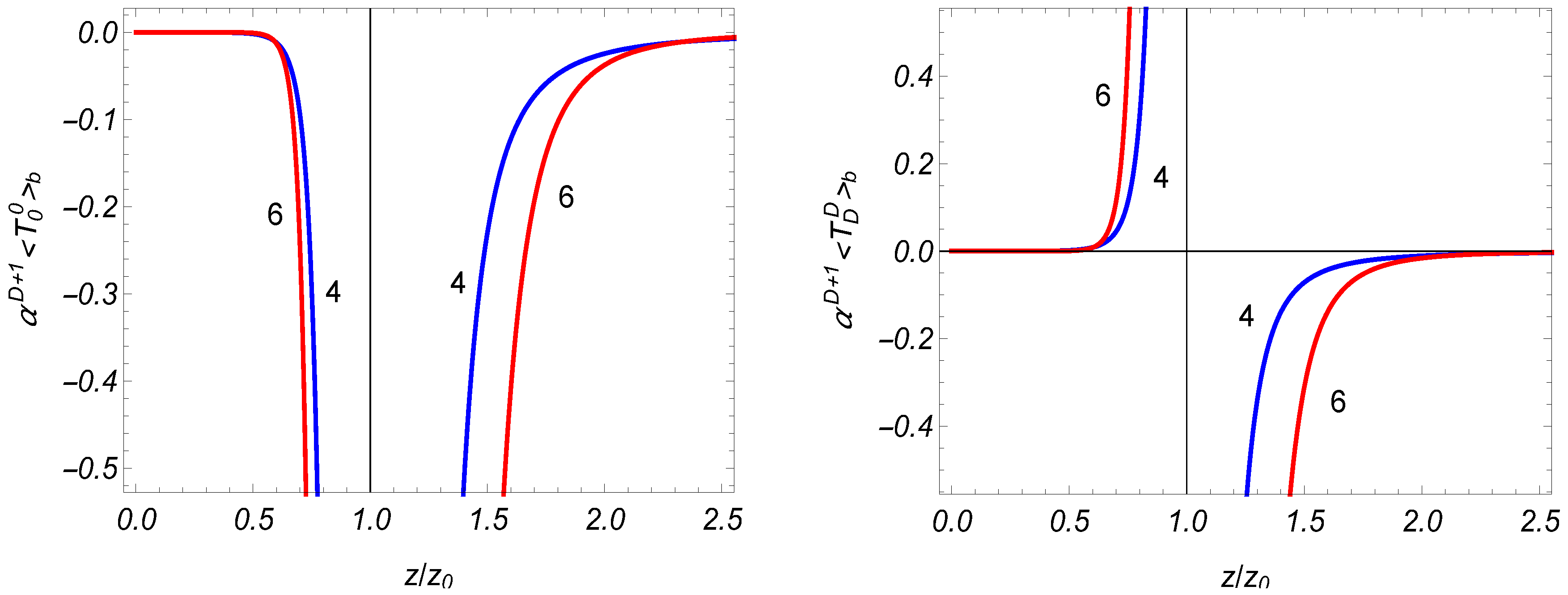
In Figure 1 we have plotted the boundary-induced contributions in the VEVs of the energy density (left panel) and the normal stress (right panel) as functions of the ratio for the number of spatial dimensions (numbers near the curves).
For the evaluation of the mode-sum (14), we have applied a variant of the generalized Abel–Plana Formula (16). That allowed us to explicitly extract the boundary-free contribution and to present the boundary-induced contribution in terms of strongly converging integral for points away from the boundary. The latter feature is related to the fact that the Abel–Plana formula automatically rotates the integration contour to the imaginary axis. With the extracted boundary-free part from the VEVs, the renormalization of local observables is reduced to that in the boundary-free geometry. Another important advantage of the procedure based on the Formula (16) is that the explicit knowledge of the eigenvalues for the quantum number is not required. Other applications of the generalized Abel–Plana formula to the Casimir effect can be found in [39]. Note that a similar procedure, widely employed for the evaluation of the global characteristics of the vacuum in the Casimir effect, is based on the argument principle (see, for example, [1,2,3]). In particular, this method has been used for the evaluation of the renormalized Casimir energy in braneworld models on AdS bulk.
4. VEV in the R-Region
Now let us consider the R-region, . In this region, the function in (6) is a linear combination of the Bessel and Neumann functions. The relative coefficient in the linear combination is determined by the boundary condition (8), and the eigenvalues of the quantum number are continuous. For the function , one gets
where
In the normalization condition, the symbol corresponds to the Dirac delta function . For the normalization coefficient, we find
For the VEV of the energy-momentum tensor, one gets (no summation over ):
with
As before, the presence of a cutoff function is assumed in (29). For , the divergences when one removes the cutoff are the same as those in the boundary-free geometry.
In order to extract the boundary-free contribution from (29), we use the relation
with and . Here , , are the Hankel functions. The part in the VEV corresponding to the first term on the right-hand side of (31) coincides with the boundary-free VEV (18). In the remaining boundary-induced part, we rotate the integration contour in the complex plane by the angle for the term and by the angle for the term . As a result, the VEV in the R-region is decomposed as (17) with the boundary-induced contribution
and with the functions
The further simplification is similar to that for the L-region, and one gets the final expression
As seen, the boundary-induced VEVs in the L- and R-regions are obtained from each other by the replacements of the modified Bessel functions.
In the special case , the boundary-induced VEV (34) vanishes in the R-region. For , all the components are negative, . For points near the boundary, , the ratio is close to 1 and the contribution of large x dominates in (34). By using the corresponding asymptotics for the modified Bessel functions, for the leading terms we obtain the expressions (24). Near the boundary, the dominant contribution to the VEV comes from wavelengths smaller than the curvature radius, and the influence of the gravity is weak.
At distances from the boundary larger than the AdS curvature radius, one has . The dominant contribution to the integral in (34) comes from small values of x. By using the corresponding asymptotic expressions for the functions and , for the leading order terms we find
with . As seen, at large distances the boundary-induced VEVs—as functions of the proper distance—are suppressed by the factor . At distances from the boundary larger than the AdS curvature radius, the effects of gravity are essential and the behavior of the VEV is completely different from that on the Minkowski bulk. In the latter case, the decay of the VEVs, as functions of , is as power law, as for the energy density and stresses parallel to the boundary.
For the R-region, the dependence of the boundary-induced energy density and the normal stress on the ratio is presented in Figure 1.
5. Applications to Randall–Sundrum Model with a Single Brane
With the results given above, we can find the Casimir densities for the electromagnetic field in Randall–Sundrum braneworld model with a single brane (RSII model) [40] (for reviews see [41,42]). The original model has been formulated on the AdS bulk with . Here we will consider the generalization for an arbitrary value of the spatial dimension. In terms of the coordinate (22), measuring the physical distance from the brane located at , the line element has the form
where . The absolute value of the y coordinate in the metric components incorporates the -symmetry with respect to the brane: the points with the coordinates y and are identified. From (36), it follows that in RSII model only the R-region of the AdS spacetime is employed. In terms of the coordinate z, the brane is located at .
The boundary conditions for fields on the brane are dictated by the -symmetry [43]. Two types of boundary conditions are realized corresponding to the even and odd fields under the -symmetry. First let us consider the case of odd fields. These fields obey the boundary condition . For the modes (6), this corresponds to the boundary condition (8). Hence, the electromagnetic Casimir densities in RSII model are obtained from the results given above for the R-region with . The only difference is that in the RSII model the integration over y in the normalization integral for the modes (6) goes over the region instead of the interval . This leads to an additional factor in the normalization coefficient for the mode functions. Consequently, the Casimir densities for odd fields in the RSII model are given by (34) with an additional factor 1/2. Note that in this case there is no Kaluza–Klein zero mode.
For even fields, the boundary condition on the brane reads . For the modes (6) it is reduced to at . By taking into account that for cylinder functions one has , this condition is rewritten as
Note that the boundary condition for even fields can be written in terms of the field tensor as . This type of boundary condition is used to confine the gluon fields in QCD (in particular, in MIT bag models). The procedure for the evaluation of the vacuum energy-momentum tensor in the R-region for this type of boundary condition is similar to that described in Section 4. We will omit the details and present the final result for the RSII model (no summation over ):
with and . As it has been explained above, the additional factor 2 in the denominator is related to the presence of two regions and for the coordinate y connected by the -symmetry. The qualitative behavior of the brane-induced energy density and the normal stress is similar to that depicted in Figure 1. Note that in [36] the Casimir energy is considered for even fields.
6. Conclusions
For -dimensional AdS spacetime, we have investigated the influence a planar boundary, parallel to the AdS horizon, on the properties of the electromagnetic vacuum. On the boundary, the electromagnetic field obeys the condition that generalizes the perfect conductor boundary condition for . As the local characteristic of the vacuum state we have considered the VEV of the energy-momentum tensor. The latter is among the most important quantities in quantum field theory on curved backgrounds. The vacuum energy-momentum tensor is diagonal, and the stresses parallel to the boundary are equal to the energy-density. The latter property is a direct consequence of the Lorentz invariance with respect to the boosts along the spatial dimensions parallel to the boundary.
The quantum properties of the vacuum are completely different for the region between the boundary and the AdS boundary (region , referred to here as the L-region) and for the region between the boundary and AdS horizon (region , referred to as the R-region). In the first region, in addition to the boundary condition at , the field operator is constrained by the boundary condition on the AdS boundary. The latter is required by the normalizability condition of the mode functions. As a consequence, in the L-region the eigenvalues of the quantum number form a discrete set determined by the zeros of the Bessel function . The mode-sum for the energy-momentum tensor contains a summation over these zeros. For the transformation of the corresponding series, we have applied the generalized Abel–Plana formula that allowed the extraction of the boundary-free part from the VEV. For points away from the boundary, the renormalization is required for that part only. The boundary-induced contribution is given by the expression (21). The vacuum energy density is negative, and the normal stress is positive. In the special case , the problem for the L-region is conformally related to the problem in Minkowski bulk with two parallel conducting plates, and for the energy-momentum tensor we have a simple result (23). In this special case, the VEV is finite on the boundary. This is not the case for , and the VEV diverges on the boundary with the leading terms given by (24). On the AdS boundary, the boundary-induced contributions vanish like . As a function of the proper distance from the AdS boundary, this corresponds to the exponential suppression by the factor with .
In the R-region, the quantum number is continuous and the boundary-induced contribution to the VEV of the energy-momentum tensor is presented as (34). Both the energy density and the normal stress are negative for . In the case , the problem in the R-region is conformally related to the Minkowskian problem with a single conducting plate, and the boundary-induced contribution vanishes. For points near the boundary, the main contribution to the VEV comes from the fluctuations with wavelengths smaller than the AdS curvature radius. The influence of the gravitational field on those fluctuations is weak and the leading terms in the asymptotic expansion coincides with those in the Minkowski bulk. The influence of the gravitational field is essential at distances from the boundary larger than the curvature radius. At large distances, the boundary-induced contribution is suppressed by the factor and it vanishes on the AdS horizon. From the expressions for the VEV of the energy-momentum tensor in the R-region, the corresponding formulas can be obtained for odd and even vector fields in Randall–Sundrum model with a single brane. For odd fields, the boundary condition on the brane is equivalent to the perfectly conducting boundary condition, and the VEV is given by (34) with and with an additional factor 1/2. The latter is related to the orbifold nature of the background in Randall–Sundrum models. For even vector fields, the boundary condition is given by (37). The latter is employed for the confinement of gluon fields in QCD. The corresponding VEV is given by the expression (38).
Acknowledgments
This work was supported by the State Committee of Science Ministry of Education and Science RA, within the frame of Grants SCS 15T-1C110 and SCS 15RF-009.
Author Contributions
The authors contributed equally to all the stages of the work reported.
Conflicts of Interest
The authors declare no conflict of interest.
References
- Elizalde, E.; Odintsov, S.D.; Romeo, A.; Bytsenko, A.A.; Zerbini, S. Zeta Regularization Techniques with Applications; World Scientific: Singapore, 1994. [Google Scholar]
- Bordag, M.; Klimchitskaya, G.L.; Mohideen, U.; Mostepanenko, V.M. Advances in the Casimir Effect; Oxford University Press: Oxford, UK, 2009. [Google Scholar]
- Dalvit, D.; Milonni, P.; Roberts, D.; da Rosa, F. Lecture Notes in Physics: Casimir Physics; Springer: Berlin, Germany, 2011; Volume 834. [Google Scholar]
- Kotanjyan, A.S.; Saharian, A.A. Electromagnetic quantum effects in anti-De Sitter spacetime. Phys. At. Nucl. 2017, 80, 562–571. [Google Scholar] [CrossRef]
- Saharian, A.A.; Setare, M.R. The Casimir effect on background of conformally flat brane-world geometries. Phys. Lett. B 2003, 552, 119–126. [Google Scholar] [CrossRef]
- Knapman, A.; Toms, D.J. Stress energy tensor for a quantized bulk scalar field in the Randall-Sundrum brane model. Phys. Rev. D 2004, 69, 044023. [Google Scholar] [CrossRef]
- Saharian, A.A. Wightman function and Casimir densities on AdS bulk with application to the Randall– Sundrum braneworld. Nucl. Phys. B 2005, 712, 196–228. [Google Scholar] [CrossRef]
- Saharian, A.A. Surface Casimir densities and induced cosmological constant on parallel branes in AdS spacetime. Phys. Rev. D 2004, 70, 064026. [Google Scholar] [CrossRef]
- Shao, S.-H.; Chen, P.; Gu, J.-A. Stress-energy tensor induced by bulk Dirac spinor in Randall-Sundrum model. Phys. Rev. D 2010, 81, 084036. [Google Scholar] [CrossRef]
- Elizalde, E.; Odintsov, S.D.; Saharian, A.A. Fermionic Casimir densities in anti-de Sitter spacetime. Phys. Rev. D 2013, 87, 084003. [Google Scholar] [CrossRef]
- Flachi, A.; Garriga, J.; Pujolàs, O.; Tanaka, T. Moduli stabilization in higher dimensional brane models. J. High Energy Phys. 2003, 8, 053. [Google Scholar] [CrossRef]
- Flachi, A.; Pujolàs, O. Quantum self-consistency of AdS × Σ brane models. Phys. Rev. D 2003, 68, 025023. [Google Scholar] [CrossRef]
- Saharian, A.A. Wightman function and vacuum fluctuations in higher dimensional brane models. Phys. Rev. D 2006, 73, 044012. [Google Scholar] [CrossRef]
- Saharian, A.A. Bulk Casimir densities and vacuum interaction forces in higher dimensional brane models. Phys. Rev. D 2006, 73, 064019. [Google Scholar] [CrossRef]
- Saharian, A.A. Surface Casimir densities and induced cosmological constant in higher dimensional braneworlds. Phys. Rev. D 2006, 74, 124009. [Google Scholar] [CrossRef]
- Elizalde, E.; Minamitsuji, M.; Naylor, W. Casimir effect in rugby-ball type flux compactifications. Phys. Rev. D 2007, 75, 064032. [Google Scholar] [CrossRef]
- Linares, R.; Morales-Técotl, H.A.; Pedraza, O. Casimir force for a scalar field in warped brane worlds. Phys. Rev. D 2008, 77, 066012. [Google Scholar] [CrossRef]
- Frank, M.; Saad, N.; Turan, I. Casimir force in Randall-Sundrum models with q + 1 dimensions. Phys. Rev. D 2008, 78, 055014. [Google Scholar] [CrossRef]
- Teo, L.P. Casimir effect in spacetime with extra dimensions–from Kaluza–Klein to Randall–Sundrum models. Phys. Lett. B 2009, 682, 259–265. [Google Scholar] [CrossRef]
- Elizalde, E.; Odintsov, S.D.; Saharian, A.A. Repulsive Casimir effect from extra dimensions and Robin boundary conditions: From branes to pistons. Phys. Rev. D 2009, 79, 065023. [Google Scholar] [CrossRef]
- Bezerra de Mello, E.R.; Saharian, A.A.; Setare, M.R. Vacuum densities for a brane intersecting the AdS boundary. Phys. Rev. D 2015, 92, 104005. [Google Scholar] [CrossRef]
- Bezerra de Mello, E.R.; Saharian, A.A.; Vardanyan, V. Induced vacuum currents in anti-de Sitter space with toral dimensions. Phys. Lett. B 2015, 741, 155–162. [Google Scholar] [CrossRef]
- Bellucci, S.; Saharian, A.A.; Vardanyan, V. Vacuum currents in braneworlds on AdS bulk with compact dimensions. J. High Energy Phys. 2015, 11, 092. [Google Scholar] [CrossRef]
- Bellucci, S.; Saharian, A.A.; Vardanyan, V. Hadamard function and the vacuum currents in braneworlds with compact dimensions: Two-brane geometry. Phys. Rev. D 2016, 93, 084011. [Google Scholar] [CrossRef]
- Bellucci, S.; Saharian, A.A.; Vardanyan, V. Fermionic currents in AdS spacetime with compact dimensions. Phys. Rev. D 2017, 96, 065025. [Google Scholar] [CrossRef]
- Durrer, R.; Ruser, M. Dynamical Casimir effect in braneworlds. Phys. Rev. Lett. 2007, 99, 071601. [Google Scholar] [CrossRef] [PubMed]
- Wilson, C.M.; Johansson, G.; Pourkabirian, A.; Simoen, M.; Hohansson, J.R.; Duty, T.; Nori, F.; Delsing, P. Observation of the dynamical Casimir effect in a superconducting circuit. Nature 2011, 479, 376–379. [Google Scholar] [CrossRef] [PubMed]
- Felicetti, S.; Sanz, M.; Lamata, L.; Romero, G.; Johansson, G.; Delsing, P.; Solano, E. Dynamical Casimir effect entangles artificial atoms. Phys. Rev. Lett. 2014, 113, 093602. [Google Scholar] [CrossRef] [PubMed]
- Hartnoll, S.A.; Herzog, C.P.; Horowitz, G.T. Building a holographic superconductor. Phys. Rev. Lett. 2008, 101, 031601. [Google Scholar] [CrossRef] [PubMed]
- García-Álvarez, L.; Egusquiza, I.L.; Lamata, L.; del Campo, A.; Sonner, J.; Solano, E. Digital quantum simulation of minimal AdS/CFT. Phys. Rev. Lett. 2017, 119, 040501. [Google Scholar] [CrossRef]
- Allen, B.; Jacobson, T. Vector Two-Point Functions in Maximally Symmetric Spaces. Commun. Math. Phys. 1986, 103, 669–692. [Google Scholar] [CrossRef]
- Saharian, A.A.; Kotanjyan, A.S.; Saharyan, A.A. Electromagnetic Casimir densities for a plate in anti-de Sitter spacetime. Phys. Math. Sci. 2016, 3, 37–41. [Google Scholar]
- Saharian, A.A.; Kotanjyan, A.S.; Nersisyan, H.A. Electromagnetic two-point functions and Casimir densities for a conducting plate in de Sitter spacetime. Phys. Lett. B 2014, 728, 141–147. [Google Scholar] [CrossRef] [Green Version]
- Kotanjyan, A.S.; Saharian, A.A.; Nersisyan, H.A. Electromagnetic Casimir effect for conducting plates in de Sitter spacetime. Phys. Scr. 2015, 90, 065304. [Google Scholar] [CrossRef]
- Bellucci, S.; Saharian, A.A. Electromagnetic two-point functions and the Casimir effect in Friedmann- Robertson-Walker cosmologies. Phys. Rev. D 2013, 88, 064034. [Google Scholar] [CrossRef]
- Teo, L.P. Casimir effect of electromagnetic field in Randall-Sundrum spacetime. J. High Energy Phys. 2010, 10, 019. [Google Scholar] [CrossRef]
- Frank, M.; Turan, I.; Ziegler, L. The Casimir force in Randall-Sundrum models. Phys. Rev. D 2007, 76, 015008. [Google Scholar] [CrossRef]
- Saharian, A.A. The generalized Abel-Plana formula. Applications to Bessel functions and Casimir effect. arXiv, 2000; arXiv:hep-th/0002239. [Google Scholar]
- Saharian, A.A. The Generalized Abel-Plana Formula with Applications to Bessel Functions and Casimir Effect; Yerevan State University Publishing House: Yerevan, Armenia, 2008. [Google Scholar]
- Randall, L.; Sundrum, R. An alternative to compactification. Phys. Rev. Lett. 1999, 83, 4690–4693. [Google Scholar] [CrossRef]
- Kiritsis, E. D-branes in standard model building, gravity and cosmology. Phys. Rep. 2005, 421, 105–190. [Google Scholar] [CrossRef]
- Maartens, R.; Koyama, K. Brane-world gravity. Living Rev. Relativ. 2010, 13, 5. [Google Scholar] [CrossRef] [PubMed]
- Gherghetta, T.; Pomarol, A. Bulk fields and supersymmetry in a slice of AdS. Nucl. Phys. B 2000, 586, 141–162. [Google Scholar] [CrossRef]
Figure 1.
The VEVs of the energy density (left panel) and of the normal stress (right panel) versus the ratio in spatial dimensions (numbers near the curves).
Figure 1.
The VEVs of the energy density (left panel) and of the normal stress (right panel) versus the ratio in spatial dimensions (numbers near the curves).
© 2017 by the authors. Licensee MDPI, Basel, Switzerland. This article is an open access article distributed under the terms and conditions of the Creative Commons Attribution (CC BY) license (http://creativecommons.org/licenses/by/4.0/).
Share and Cite
MDPI and ACS Style
Kotanjyan, A.S.; Saharian, A.A.; Saharyan, A.A. Electromagnetic Casimir Effect in AdS Spacetime. Galaxies 2017, 5, 102. https://doi.org/10.3390/galaxies5040102
AMA Style
Kotanjyan AS, Saharian AA, Saharyan AA. Electromagnetic Casimir Effect in AdS Spacetime. Galaxies. 2017; 5(4):102. https://doi.org/10.3390/galaxies5040102
Chicago/Turabian StyleKotanjyan, Anna S., Aram A. Saharian, and Astghik A. Saharyan. 2017. "Electromagnetic Casimir Effect in AdS Spacetime" Galaxies 5, no. 4: 102. https://doi.org/10.3390/galaxies5040102
Note that from the first issue of 2016, this journal uses article numbers instead of page numbers. See further details here.