
Modeling the Time-Dependent Polarization of Blazars


1
Institute for Astrophysical Research, Boston University, 725 Commonwealth Ave., Boston, MA 02215, USA
2
Astronomical Institute, St. Petersburg State University, Universitetsky Prospekt, 28, Petrodvorets, 198504 St. Petersburg, Russia
*
Author to whom correspondence should be addressed.
Galaxies 2017, 5(4), 63; https://doi.org/10.3390/galaxies5040063
Submission received: 21 September 2017
/
Revised: 6 October 2017
/
Accepted: 9 October 2017
/
Published: 13 October 2017
(This article belongs to the Special Issue Polarised Emission from Astrophysical Jets)
Abstract
:Linear polarization is an extremely valuable observational tool for probing the dynamic physical conditions of blazar jets. Some patterns are seen in the data, suggestive of order that can be explained by shock waves and helical magnetic field components. However, much disorder is apparent, which implies that turbulence plays a major role as well, especially in the fluctuations of flux and polarization, and perhaps particle acceleration. Here, we present some actual flux and polarization versus time data, plus simulations of model jets. We analyze the output of the simulations in a manner that can be compared with observational data. The results suggest that the ratio of turbulent to ordered magnetic fields varies with time.
1. Introduction
Magnetic fields play a critical role in various aspects of the physics of relativistic jets. Dominance of magnetic over rest-mass energy at the base of a jet is required in order to accelerate plasmas almost to the speed of light, the natural velocity of dynamic electromagnetic phenomena. Energization of charged particles to GeV-TeV levels must also involve electromagnetic fields that vary over time and space. The synchrotron radiation emitted by jets from radio to UV, or even X-ray, frequencies involves energetic electrons spiraling in magnetic fields. However, it is challenging to determine the geometry of magnetic fields in cosmic jets lying at distances too remote for in situ measurements. For this, we rely on observations of the polarization.
We, along with a number of collaborators, are engaged in studies of the time-variable structure of the emission and linear polarization of the relativistic jets of blazars. The methods that we employ include Very Long Baseline Interferometry (VLBI), mostly at a frequency of 43 GHz with the Very Long Baseline Array (VLBA), multi-frequency monitoring of the total flux density, and—at millimeter to optical wavelengths—degree P and position angle χ of linear polarization. In general, both P and χ are highly variable, and thus can only be properly interpreted via descriptions that involve dynamical processes. In what follows, the authors present ideas and calculations that attempt to provide such descriptions. This is a work in progress, so this paper reports on preliminary results. More quantitative conclusions must await more comprehensive studies by the authors, and perhaps by others.
2. Observations of Optical Polarization of Blazars
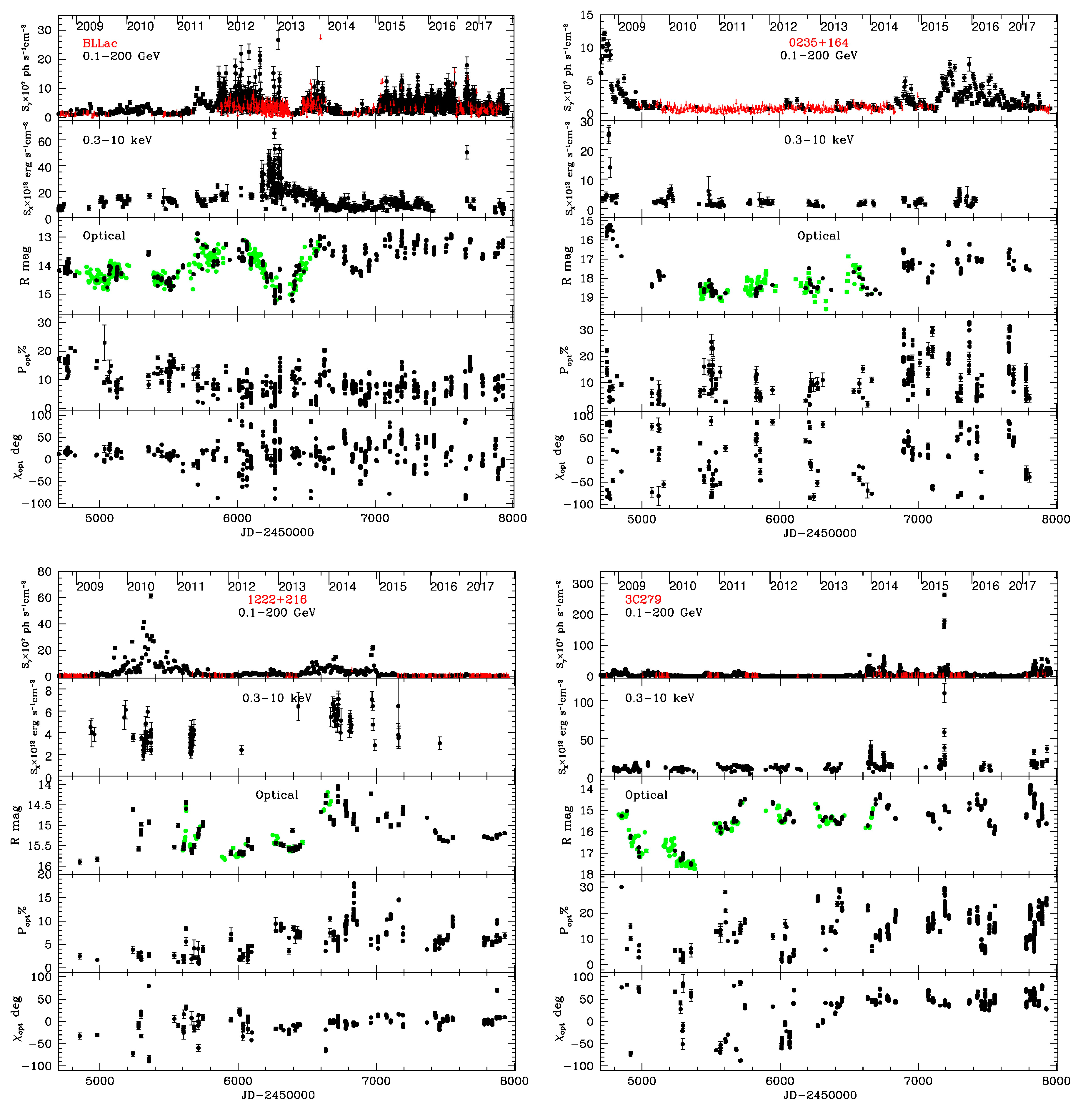
Before attempting to use polarization as a probe of the physical conditions of blazar jets, it is instructive to examine observed polarization vs. time curves, some of which we display in Figure 1 (see Supplementary Materials). The optical polarization data were obtained by us with the 1.8-m diameter Perkins Telescope of Lowell Observatory in Flagstaff, AZ, USA. Also shown are γ-ray fluxes and upper limits from the Large Area Telescope of the Fermi Gamma-ray Space Telescope, X-ray fluxes measured with the XRT detector of the Swift satellite observatory, and optical fluxes (in green) obtained with the 2.0-m diameter Liverpool Telescope at the Observatorio del Roque de Los Muchachos on the Canary Island of La Palma, Spain (I. M. McHardy was the principal investigator of the program). Details of the observations and data analysis can be found in Jorstad et al. [1]
The temporal behavior of the four blazars appears to be a mixture of randomness and systematic patterns. However, these patterns only occur some of the time, and are not common to all of the objects. This is in keeping with a primary characteristic of blazars: their extreme variability. For example, during the relatively quiescent period before early 2011, the optical polarization of BL Lacertae varied in degree by up to ~30%, while χ remained roughly steady at ~20°, which is close to the parsec-scale jet direction as seen in 43 GHz VLBA observations. After this period, the jet became more active, with χ executing pronounced variations. One can conclude that a process, such as turbulence, that causes disorder in the magnetic field operates during multi-flare outbursts, but is dominated by a more uniform magnetic field—possibly helical or shock-compressed—during quiescence. The polarization variations, however, had the opposite tendency in the BL Lac object 0235+164: modest fluctuations in χ during quiet periods and keeping within ~20° of the inner jet direction most of the time during periods of high activity. The quasar 3C 279 maintained a nearly constant value of χ close to the parsec-scale jet direction much of the time, including the entire time-span of its most pronounced γ-ray and X-ray activity (late 2013 to mid-2015), but χ also varied wildly during some quiet and relatively active periods. The behavior of χ was somewhat similar in the quasar 1222+216 (4C 21.35), with wild variations during the strongest γ-ray outburst in 2010 and near-constancy along the direction of the inner jet during a second pronounced outburst in 2013–2015.
The degree of polarization P, on the other hand, varied strongly at nearly all times in all four blazars. This leads to the strong conclusion that there is significant disorder in the magnetic field in the emission zone of blazars at essentially all times. This statement is supported by the relatively low value of P, which is always much less than the value of ~70–75% of synchrotron radiation from a region of uniform magnetic field. A common cause of disorder in cosmic magnetic fields is turbulence. Yet the constancy of χ some of the time requires the action of a process that partially orders the magnetic field as well, e.g., shocks or a helical magnetic field pattern superposed on the turbulence. Even for a completely disordered magnetic field, relativistic aberration of radiation from disordered field in a nearly cylindrical jet can yield a net linear polarization with χ parallel to the jet axis. These considerations have inspired the lead author to develop a numerical model of blazar emission (Turbulent Extreme Multi-Zone model, or TEMZ [2]) that includes the effects of turbulence, shocks, helical magnetic fields, and aberration. The remainder of this paper summarizes the model and some of the preliminary findings that it has produced.
3. Model for Calculating the Time-Variable Polarized Emission from Relativistic Jets
In order to simulate the effects of turbulence as well as variable input of energy into the base of the jet, TEMZ utilizes a modification of the nested-cells scheme of Jones [3]. The jet is divided into many cylindrical cells, while the cells are each a member of 4 nested zones, one containing only that cell, and the others containing 8, 64, and 512 cells. Each zone possesses a uniform magnetic field (with random direction) and density, selected from a log-normal probability distribution with standard deviation equal to 0.4 times the mean value, the latter of which is a free parameter guided by observations of turbulence in the solar wind (e.g., [4]). The contribution of each zone to a cell’s magnetic and particle energy densities follows a Kolmogorov spectrum, with a u ∝ x−2/3 law, where x is the dimension of the zone. In order to reproduce the long time-scale variability of the emission from the blazar, the mean energy density in relativistic electrons injected into the jet’s base is modulated at random with a red-noise power spectrum.
The TEMZ code calculates the nonthermal emission over a cylindrical section of the jet that is intended to represent the “core” seen on VLBI images at millimeter wavelengths, but could also correspond to quasi-stationary emission features downstream of the core. The upstream boundary of the region can either be a conical “recollimation” shock that accelerates electrons to highly relativistic energies as plasma crosses the shock front, or simply a turbulent zone. In the former case, the emission region is truncated at the downstream end by a conical rarefaction wave, beyond which the emission is assumed to be negligible because of a magnetic field strength, density, and mean electron energy that is considerably lower than in the shocked region. In the simple turbulent zone, the emission occurs throughout a cylindrical volume, with electrons either accelerated only at the upstream boundary (e.g., via many magnetic reconnections) or throughout the volume (e.g., via second-order Fermi acceleration and/or many magnetic reconnections in the turbulent plasma). After attaining a power-law energy distribution, the electrons lose energy to synchrotron and inverse Compton losses.
In the case of the standing shock scenario, the power-law distribution of electron energies endowed by the code extends up to some value γmax,min mc2 unless the magnetic field of the turbulent cell happens to be nearly parallel to the shock normal (referred to as the “subluminal” case of particle acceleration; see, e.g., [5]). In this case, the energy distribution extends to a higher value, γmax,max mc2. Since very high electron energies (γ > 3000) are required to generate optical to X-ray synchrotron radiation and GeV-TeV inverse Compton γ rays for ~0.1–1 G magnetic fields, emission at these frequencies has a smaller volume-filling factor than that at lower frequencies. This causes a steepening of the spectrum toward higher frequencies, which is an alternative to a double power-law with a sharp break or log-parabola electron energy distribution, each of which has been popular with modelers. The smaller volume also allows the higher-frequency flux and polarization to vary more rapidly than at lower frequencies.
Sample simulated light curves produced by the TEMZ model can be found in [1,6,7]. Here, we concentrate on simulations of the linear polarization behavior of blazars for different mixtures of turbulent and helical magnetic fields in the emission zone under the shock and no-shock scenarios. The goal is to provide statistical tests that can differentiate among the various physical possibilities. All of the simulations presented here adopt an ambient (i.e., pre-shock) bulk Lorentz factor Γ = 6 and a viewing angle of 3° to the jet axis, or about 0.5 arcsin (1/Γ) that should be typical for γ-ray bright blazars. The lead author plans a more thorough exploration of parameter space in the future.
3.1. 100% Turbulent Magnetic Field
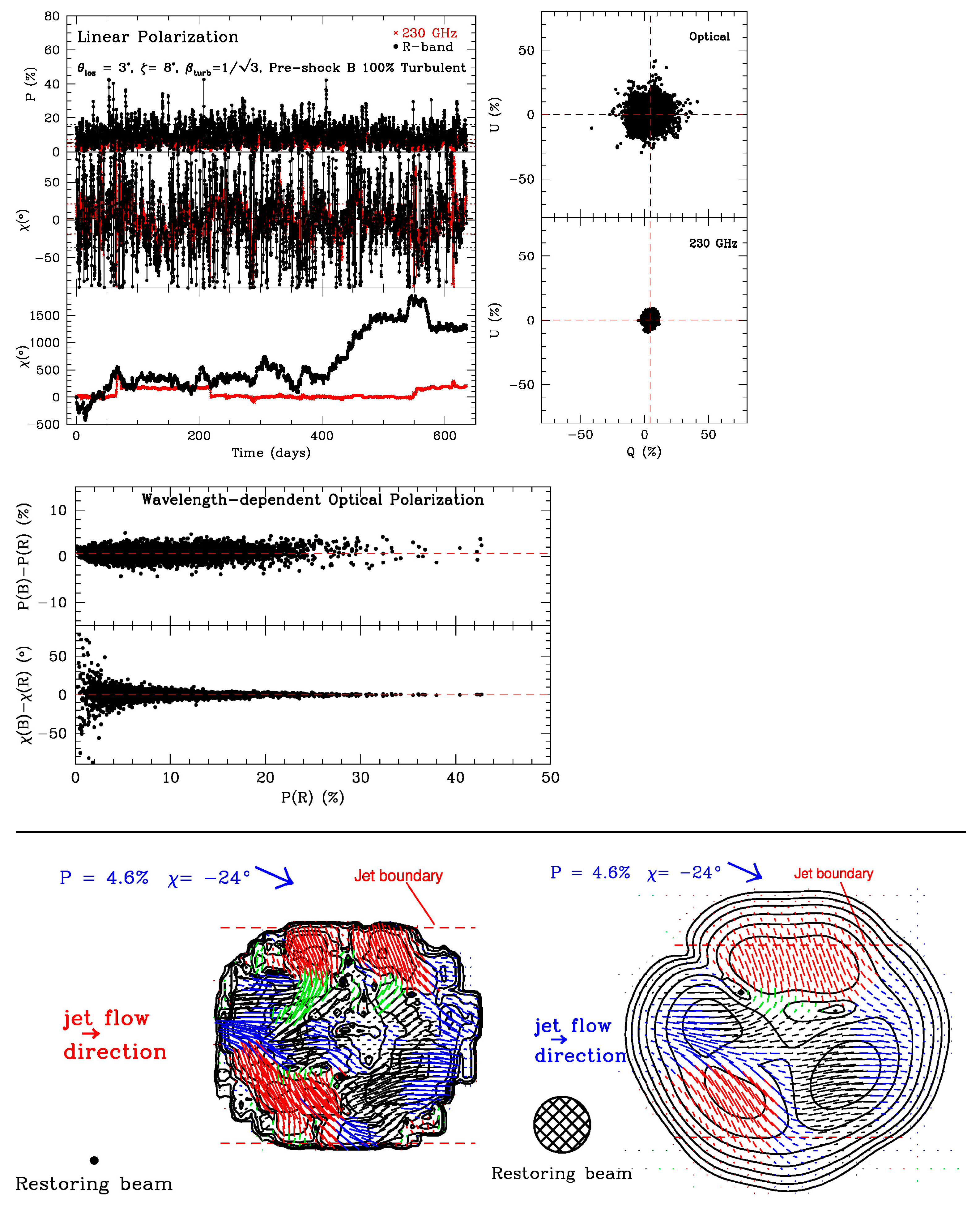
When there is neither an ordered component to the magnetic field in the ambient jet nor a shock, the linear polarization is governed by random behavior. Figure 2 presents results for the case when electrons are continuously energized in each cell. In the polarization vs. time plots in this and subsequent figures, the middle panel displays the electric-vector position angle χ constrained to the range of −90° to +90°, while the bottom panel determines the value of χ by forcing the change between time steps to be less than 90°. The latter allows apparent rotations of χ exceeding 180°, but gives the odd result that the 230 GHz and optical values of χ diverge, while in the −90° to +90° plot they usually track each other quite well. This sensitivity to the algorithm for dealing with changes in χ has been noted by Kiehlmann et al. [8]. The mean optical polarization is higher than that at 230 GHz because fewer cells have electrons with sufficient energies to radiate strongly at optical frequencies, since this requires a value of Bsinφ’ that is only attained by some of the cells, where B is the magnetic field strength and φ’ is the angle between the line of sight and magnetic field direction in the (aberrated) plasma frame. The mean degree of polarization is inversely proportional to the square-root of the number of cells with independent magnetic field directions that contribute to the emission [9]. This effect causes the degree of polarization to fail to exceed 10% over the 5000 time steps of the simulation; despite the linkage of larger to smaller scales by the Kolmogorov spectrum of the turbulence, the number of essentially independent magnetic field directions remains high. This can be visualized in the bottom-left simulated 230 GHz image in Figure 2, convolved with a tiny restoring beam that allows small regions of various values of χ to be apparent. Of more practical use is the bottom-right image, convolved with a 20 microarcsecond beam typical of VLBI at 1.3 mm. Even at this coarser resolution, several regions with very different values of χ stand out; this pattern should change across well-separated epochs owing to the randomness of the turbulent field. Note that the mean of the Q vs. U scatter plot in Figure 2 is zero, in concert with the random behavior. Finally, there is a systematically higher degree of polarization toward higher frequencies.
3.2. Turbulent Field with a Standing Shock
Figure 3 presents similar graphics for the case where plasma with 100% turbulent field crosses a conical standing shock front that partially orders the field and compresses both the field and the density of particles. Perhaps surprisingly, the level of order does not decrease the complexity of the polarization vs. time behavior. Rather, the degree of polarization fluctuates more wildly, with a higher mean value and occasional peaks above 40%, more in line with the data displayed in Figure 1 than for the case with no shock. The partial ordering causes the mean value of Q to be a few percent at both optical and 230 GHz frequencies, while that of U remains at zero. Displacement of <Q> while <U> remains close to zero corresponds to the “preferred” range of χ of 0° ± 20° apparent in the upper-left graph of the temporal behavior plotted in Figure 3, where χ = 0 corresponds to the electric vector lying parallel to the jet axis. Although color-dependent polarization occurs, the signs of the (B − R) values fluctuate, with only a statistical preference for higher percentage at higher frequencies. The images show signs of symmetry—see also [10,11]—although the pattern still changes across epochs.
3.3. Combined Turbulent and Helical Magnetic Field with a Standing Shock
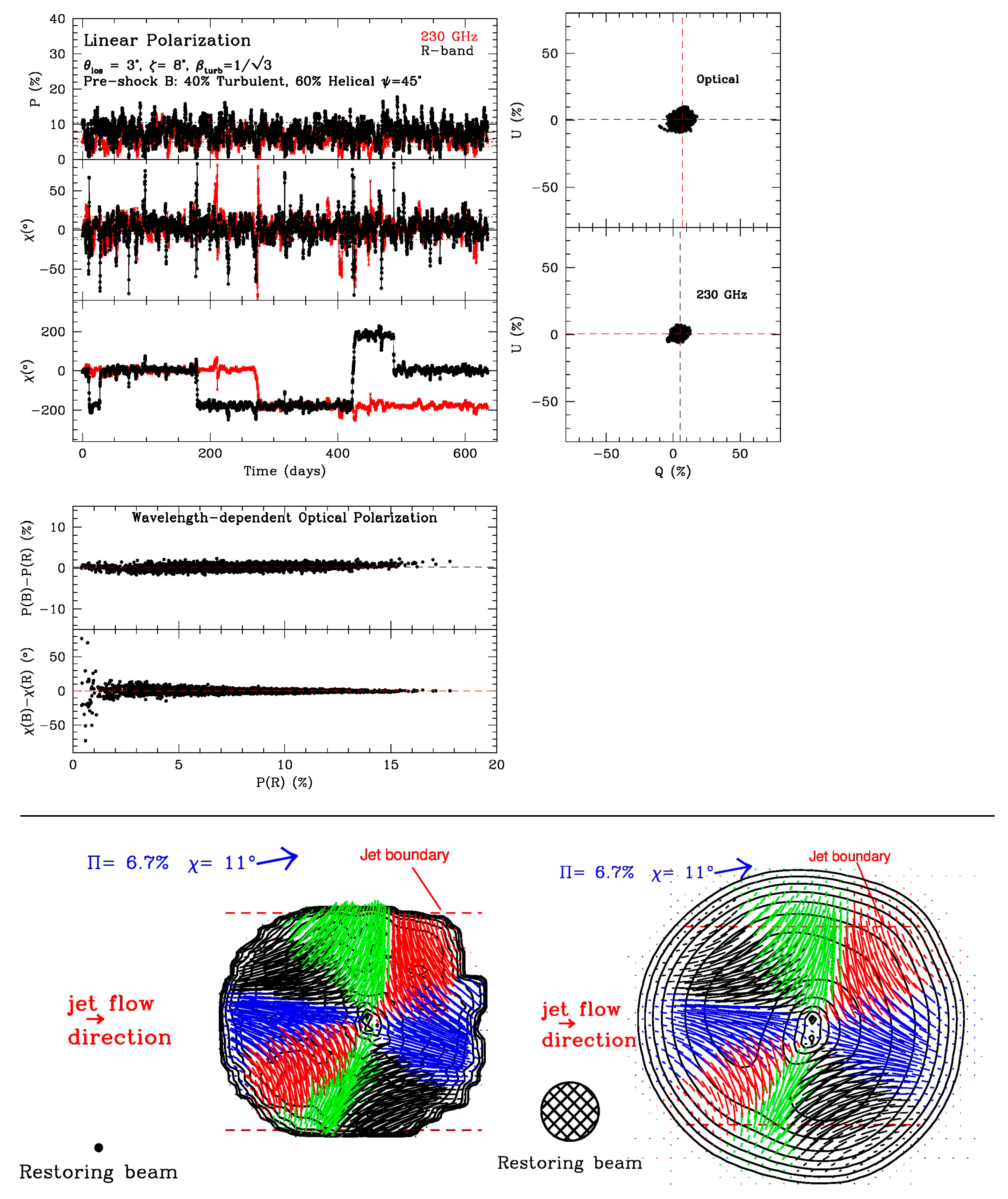
As a final example, Figure 4 presents a case where the strength of a helical magnetic field is substantial, 60% of the total mean pre-shock field. The mean of the Q vs. U scatter plot is shifted even more, to <Q> = 7% (optical) and 5% (230 GHz) while <U> = 0, than for 100% turbulent plasma crossing the shock. In addition, the scatter plot is elongated diagonally, which implies that the fluctuations in χ have a systematic component owing to the helical field component, favoring small positive values over small negative ones. (The mean value of χ is +2°.) The value of χ rarely strays beyond ±30° of the jet direction, although occasional rapid rotations occur, usually by ~180° but once by ~360°. The 230 GHz simulated polarized intensity images display a higher degree of symmetry than for the case of 100% turbulent field crossing a standing shock (Figure 3). As with that case, but less pronounced, the optical polarization has a dependence on wavelength that varies from stronger at shorter wavelengths to vice versa, with the former occurring more frequently at high polarization levels.
4. Conclusions
As one might expect, the behavior of the linear polarization of a model jet changes as one considers cases with and without a shock and with varying contributions of turbulent and ordered magnetic field in the unshocked jet plasma. Here, we have analyzed the results of simulations with the TEMZ model of three diverse cases, demonstrating that polarized intensity images at millimeter wavelengths and statistics of the time-dependent polarization at both millimeter and optical wavelengths are capable of discerning among the various physical scenarios. Comparison of Figure 2, Figure 3 and Figure 4 with Figure 1 suggests that blazar jets may alternate between turbulent-dominated and more ordered magnetic fields. An expanded exploration of the parameter space of the model is underway, with the expectation that it will lead to quantitative criteria that can be used to match the observed polarization data of a blazar with a particular set of model parameters. The ultimate goal is to describe the physical processes that control the jets and their emission.
Supplementary Materials
VLBA data and images with polarization information at many epochs, as well as multi-waveband light curves, of 37 γ-ray bright blazars and radio galaxies, are publicly available online at www.bu.edu/blazars/VLBAproject.html. Multi-color optical polarization data are listed online at www.bu.edu/blazars/mobpol.html.
Acknowledgments
The work described here was supported by US National Science Foundation grant AST-1615796 and NASA grants NNX14AQ58G (Fermi) and NNX15AR45G (Swift). A.P.M. received travel support from RadioNet. RadioNet has received funding from the European Union’s Horizon 2020 research and innovation program under grant agreement No. 730562.
Author Contributions
S.G.J. performed the optical observations at Lowell observatory, analyzed the optical data displayed in Figure 1, and arranged for some of the X-ray observations with Swift by submitting target-of-opportunity requests. K.E.W. analyzed the Fermi and Swift data displayed in Figure 1. A.P.M. created the TEMZ code and analyzed the results of running it, which are displayed in Figure 2, Figure 3 and Figure 4. In addition, he wrote the paper.
Conflicts of Interest
The authors declare no conflict of interest.
References
- Jorstad, S.G.; Marscher, A.P.; Larionov, V.M.; Agudo, L.; Smith, P.S.; Gurwell, M.; Lähteenmäki, A.; Tornikoski, M.; Markowitz, A.; Arkharov, A.A.; et al. Flaring Behavior of the Quasar 3C 454.3 across the Electromagnetic Spectrum. Astrophys. J. 2010, 715, 362–384. [Google Scholar] [CrossRef]
- Marscher, A.P. Turbulent, Extreme Multi-Zone Model for Simulating Flux and Polarization Variability in Blazars. Astrophys. J. 2014, 780, 87. [Google Scholar] [CrossRef]
- Jones, T.W. Polarization as a Probe of Magnetic Field and Plasma Properties of Compact Radio Sources—Simulation of Relativistic Jets. Astrophys. J. 1988, 332, 678–695. [Google Scholar] [CrossRef]
- Petrosyan, A.; Balogh, A.; Goldstein, M.L.; Léorat, J.; Marsch, E.; Petrovay, K.; Roberts, B.; von Steiger, R.; Vial, J.C. Turbulence in the Solar Atmosphere and Solar Wind. Space Sci. Rev. 2010, 156, 135–238. [Google Scholar] [CrossRef]
- Summerlin, E.J.; Baring, M.G. Diffusive Acceleration of Particles at Oblique, Relativistic, Magnetohydrodynamic Shocks. Astrophys. J. 2012, 745, 63. [Google Scholar] [CrossRef]
- Marscher, A.P. Time-variable Linear Polarization as a Probe of the Physical Conditions in the Compact Jets of Blazars. In Extragalactic Jets from Every Angle, IAU Symposium 313; Massaro, F., Cheung, C.C., Lopez, E., Siemiginowska, A., Eds.; Cambridge University Press: Cambridge, UK, 2015; pp. 122–127. [Google Scholar]
- Marscher, A.P. Multi-wavelength Behavior of Blazars: Combined Order & Disorder. In Proceedings of the 4th Annual Conference on High Energy Astrophysics in Southern Africa (HEASA 2016), Cape Town, South Africa, 13 January 2016. [Google Scholar]
- Kiehlmann, S.; Savolainen, T.; Jorstad, S.G.; Sokolovsky, K.V.; Schinzel, F.K.; Marscher, A.P.; Larionov, V.M.; Agudo, I.; Akitaya, H.; Benítez, E.; et al. Polarization Swings in Blazars: The Case of 3C~279. Astron. Astrophys. 2016, 590, A10–A29. [Google Scholar] [CrossRef]
- Burn, B.J. On the Depolarization of Discrete Radio Sources by Faraday Dispersion. Mon. Not. R. Astron. Soc. 1977, 133, 67–83. [Google Scholar] [CrossRef]
- Cawthorne, T.V. Polarization of Synchrotron Radiation from Conical Shock Waves. Mon. Not. R. Astron. Soc. 2006, 367, 851–859. [Google Scholar] [CrossRef]
- Cawthorne, T.V.; Jorstad, S.G.; Marscher, A.P. Evidence for Recollimation Shocks in the Core of 1803+784. Astrophys. J. 2013, 772, 14. [Google Scholar] [CrossRef]
Figure 1.
Top to bottom: 0.1–200 GeV γ-ray (units of 10−7 phot s−1 cm−2), 0.3–10 keV X-ray (10−12 erg s−1 cm−2), optical R-band magnitude, R-band degree (%), and R-band position angle (°) of optical polarization, respectively, versus time of (top) two low-synchrotron-peak BL Lac objects and (bottom) two quasars. Green symbols of optical fluxes: measurements with the Liverpool Telescope; all other optical measurements are with the Perkins Telescope.

Figure 2.
Simulated linear polarization behavior over 5000 time steps generated by the TEMZ model for the case of 100% turbulent magnetic field, no shock, and acceleration of electrons in each of 18,816 cells. Upper (left) polarization vs. time; upper (right) Stokes Q vs. U scatter plot; (middle) color-dependence (B band minus R band) of the optical polarization (dashed lines in upper right and middle plots indicate the mean values); (bottom) sample simulated maps of 230 GHz polarized intensity with polarization vectors superposed, convolved with circular Gaussian restoring beams of (left) 2 and (right) 20 microarcseconds FWHM, the former to show the underlying structure and the latter to approximate the resolution of VLBI at 230 GHz. In the images, the polarization vectors are color-coded according to the 45-degree-wide range in which they fall, for ease of visualization. In this and subsequent figures, βturb is the randomly directed velocity (in units of the speed of light) of the turbulent cells.
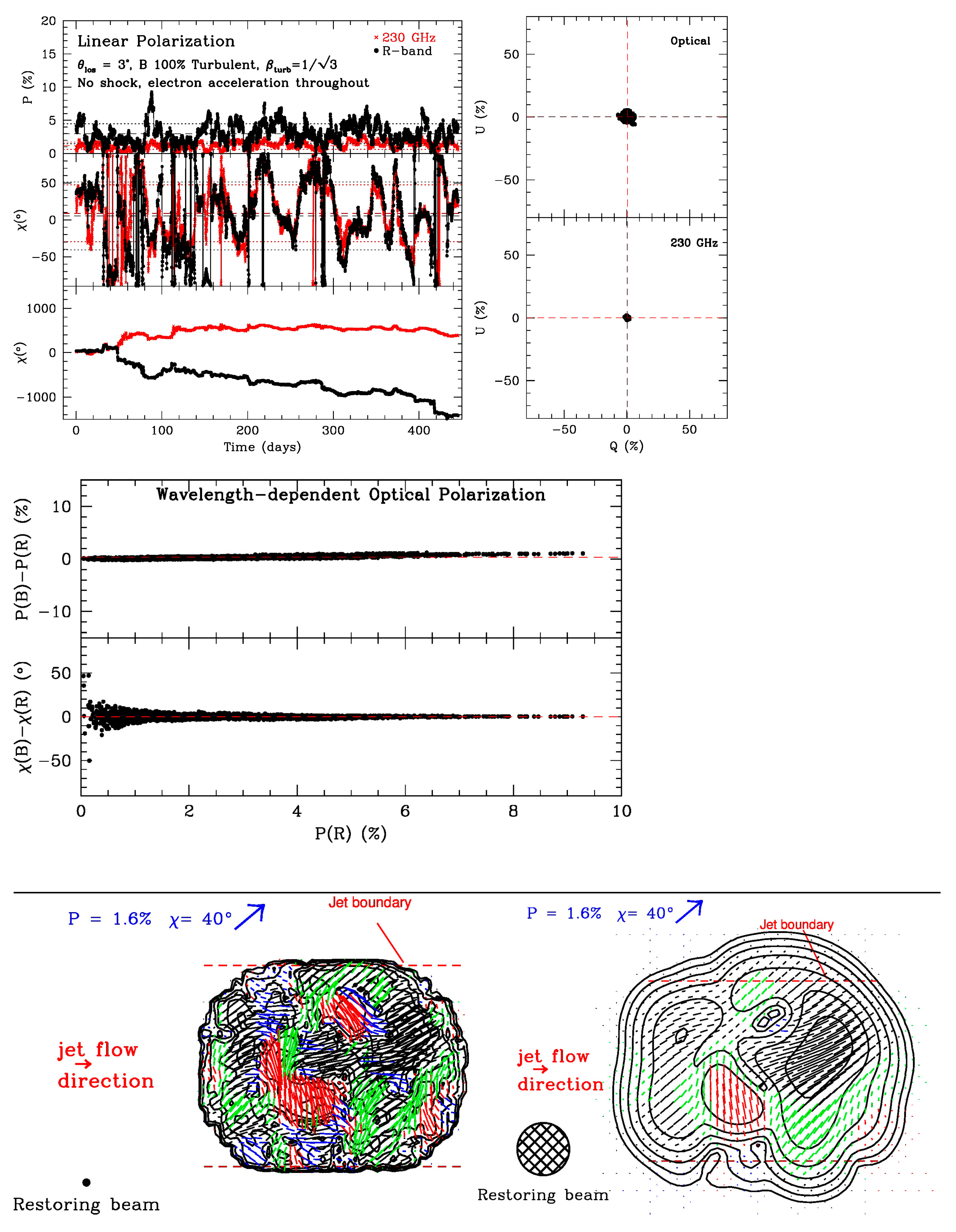
Figure 3.
Same as in Figure 2, but for the case of a conical standing shock (inclined at angle ζ = 8° to the jet axis) through which plasma with 100% turbulent magnetic field passes.
Figure 3.
Same as in Figure 2, but for the case of a conical standing shock (inclined at angle ζ = 8° to the jet axis) through which plasma with 100% turbulent magnetic field passes.

Figure 4.
Same as Figure 3, but for the case of the mean magnetic field composed of a 40% turbulent component and 60% helical component with a pitch angle ψ = 45°.
Figure 4.
Same as Figure 3, but for the case of the mean magnetic field composed of a 40% turbulent component and 60% helical component with a pitch angle ψ = 45°.
© 2017 by the authors. Licensee MDPI, Basel, Switzerland. This article is an open access article distributed under the terms and conditions of the Creative Commons Attribution (CC BY) license (http://creativecommons.org/licenses/by/4.0/).
Share and Cite
MDPI and ACS Style
Marscher, A.P.; Jorstad, S.G.; Williamson, K.E. Modeling the Time-Dependent Polarization of Blazars. Galaxies 2017, 5, 63. https://doi.org/10.3390/galaxies5040063
AMA Style
Marscher AP, Jorstad SG, Williamson KE. Modeling the Time-Dependent Polarization of Blazars. Galaxies. 2017; 5(4):63. https://doi.org/10.3390/galaxies5040063
Chicago/Turabian StyleMarscher, Alan P., Svetlana G. Jorstad, and Karen E. Williamson. 2017. "Modeling the Time-Dependent Polarization of Blazars" Galaxies 5, no. 4: 63. https://doi.org/10.3390/galaxies5040063
Note that from the first issue of 2016, this journal uses article numbers instead of page numbers. See further details here.