Intra-Night Variability of OJ 287 with Long-Term Multiband Optical Monitoring

 ,
,
Abstract
:1. Introduction
2. Observations and Data Reduction
3. Results
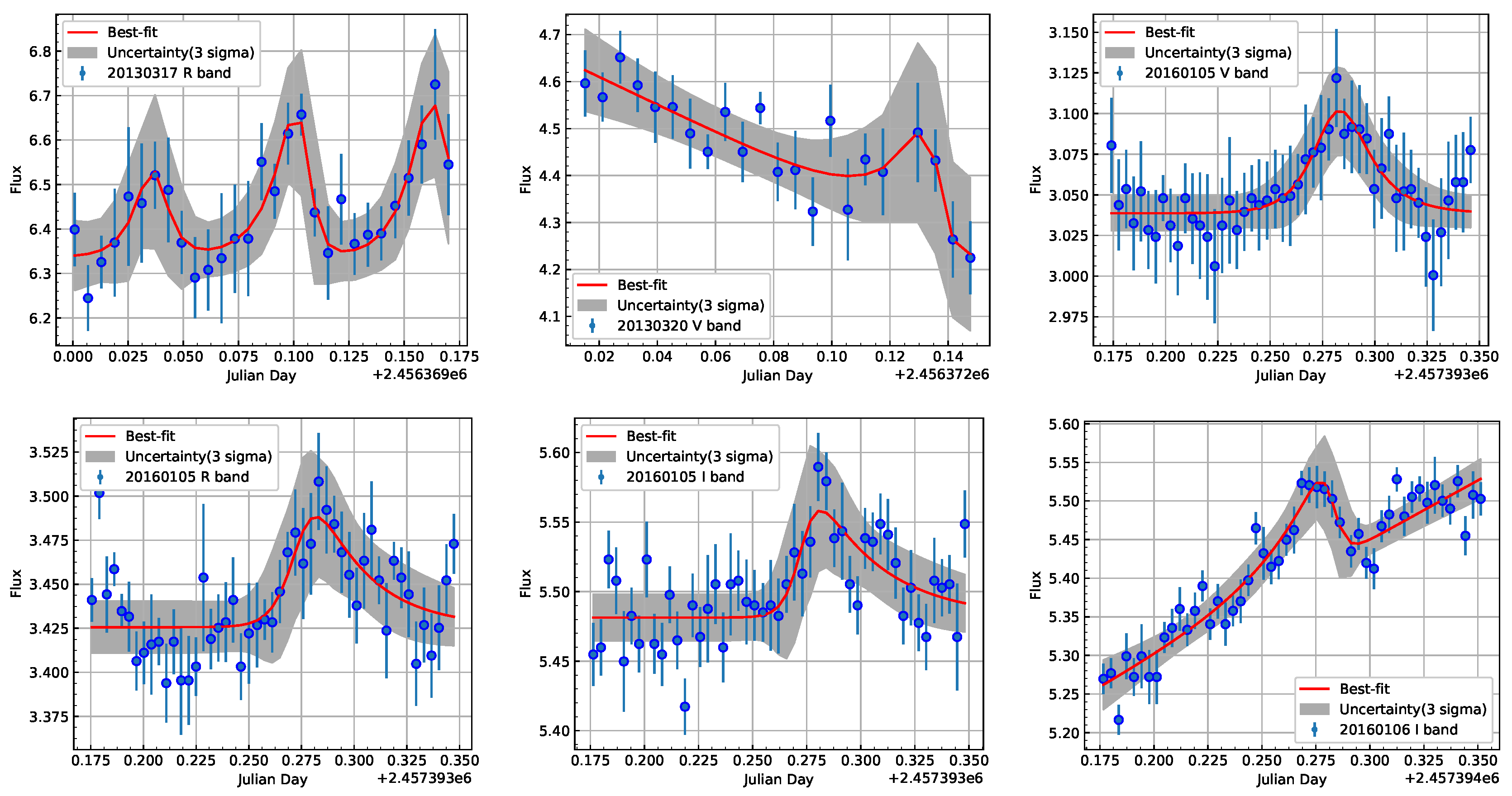
3.1. Variability
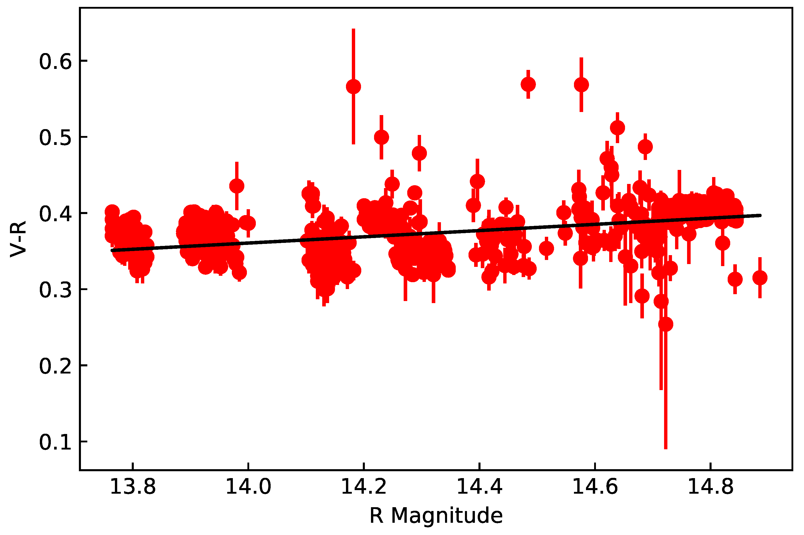
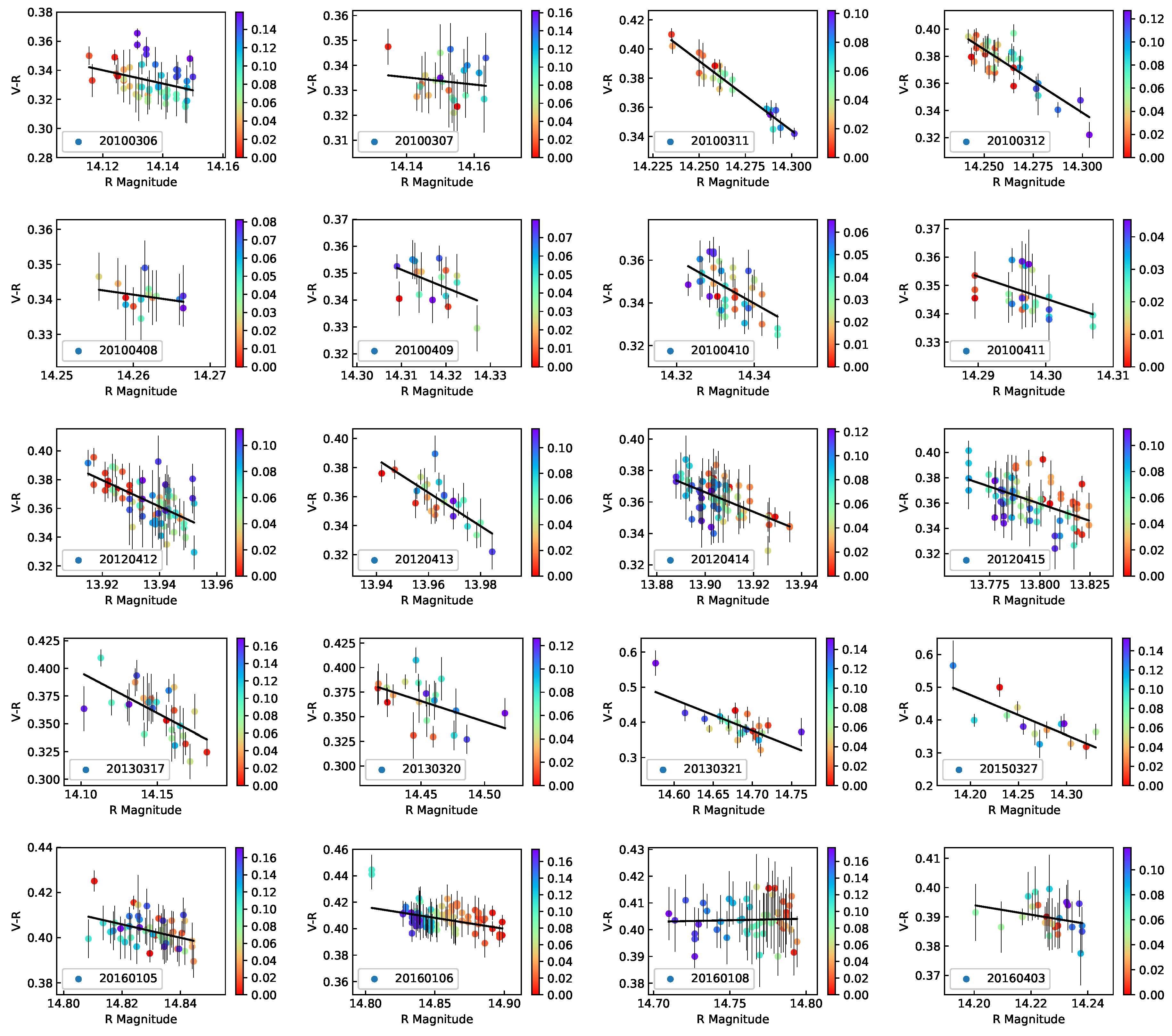
3.2. Colour Index
4. Discussion and Conclusions
Acknowledgments
Author Contributions
Conflicts of Interest
References
- Stocke, J.T.; Morris, S.L.; Gioia, I.M.; Maccacaro, T.; Schild, R.; Wolter, A.; Fleming, T.A.; Henry, J.P. The Einstein Observatory Extended Medium-Sensitivity Survey. II—The optical identifications. Astrophys. J. Suppl. Ser. 1991, 76, 813–874. [Google Scholar] [CrossRef]
- Blandford, R.D.; Rees, M.J. Extended and compact extragalactic radio sources—Interpretation and theory. Phys. Scr. 1978, 17, 265–274. [Google Scholar] [CrossRef]
- Ghisellini, G.; Villata, M.; Raiteri, C.M.; Bosio, S.; de Francesco, G.; Latini, G.; Maesano, M.; Massaro, E.; Montagni, F.; Nesci, R.A. Optical-IUE observations of the gamma-ray loud BL Lacertae object S5 0716+714: Data and interpretation. Astron. Astrophys. 1997, 327, 61–71. [Google Scholar]
- Urry, C.M.; Padovani, P. Unified Schemes for Radio-Loud Active Galactic Nuclei. Publ. Astron. Soc. Pac. 1995, 107, 803–845. [Google Scholar] [CrossRef]
- Wagner, S.J.; Witzel, A. Intraday Variability in Quasars and BL Lac Objects. Ann. Rev. Astron. Astrophys. 1995, 33, 163–198. [Google Scholar] [CrossRef]
- Goyal, A.; Wiita, P.J.; Anupama, G.C.; Sahu, D.K.; Sagar, R.; Joshi, S. Intra-night optical variability of core dominated radio quasars: The role of optical polarization. Astron. Astrophys. 2012, 544, 37–64. [Google Scholar] [CrossRef]
- Gupta, A.C.; Banerjee, D.P.K.; Ashok, N.M.; Joshi, U.C. Near infrared intraday variability of Mrk 421. Astron. Astrophys. 2004, 422, 505–508. [Google Scholar] [CrossRef]
- Fan, J.H.; Zhang, Y.W.; Qian, B.C.; Tao, J.; Liu, Y.; Hua, T.X. Photometric Monitoring of OJ 287 from 2002 to 2007. Astrophys. J. Suppl. Ser. 2009, 181, 466–472. [Google Scholar] [CrossRef]
- Dai, B.Z.; Zeng, W.; Jiang, Z.J.; Fan, Z.H.; Hu, W.; Zhang, P.F.; Yang, Q.Y.; Yan, D.H.; Wang, D.; Zhang, L. Long-term Multi-band Photometric Monitoring of Blazar S5 0716+714. Astrophys. J. Suppl. Ser. 2015, 218, 18–39. [Google Scholar] [CrossRef]
- Gupta, A.C.; Agarwal, A.; Mishra, A.; Gaur, H.; Wiita, P.J.; Gu, M.F.; Kurtanidze, O.M.; Damljanovic, G.; Uemura, M.; Semkov, E.; et al. Multiband optical variability of the blazar OJ 287 during its outbursts in 2015–2016. Mon. Not. R. Astron. Soc. 2017, 465, 4423–4433. [Google Scholar] [CrossRef]
- Sitko, M.L.; Junkkarinen, V.T. Continuum and line fluxes of OJ287 at minimum light. Publ. Astron. Soc. Pac. 1985, 97, 1158–1162. [Google Scholar] [CrossRef]
- Sillanpää, A.; Haarala, S.; Valtonen, M.J.; Sundelius, B.; Byrd, G.G. OJ 287—Binary pair of supermassive black holes. Astrophys. J. 1988, 325, 628–634. [Google Scholar] [CrossRef]
- Sillanpää, A.; Takalo, L.O.; Pursimo, T.; Lehto, H.J.; Nilsson, K.; Teerikorpi, P.; Heinaemaeki, P.; Kidger, M.; De Diego, J.A.; Gonzalez-Perez, J.N.; et al. Confirmation of the 12-year optical outburst cycle in blazar OJ 287. Astron. Astrophys. 1996, 305, 17–20. [Google Scholar]
- Sillanpää, A.; Takalo, L.O.; Pursimo, T.; Nilsson, K.; Heinamaki, P.; Katajainen, S.; Pietila, H.; Hanski, M.; Rekola, R.; Kidger, M.; et al. Double-peak structure in the cyclic optical outbursts of blazar OJ 287. Astron. Astrophys. 1996, 315, 13–16. [Google Scholar]
- Valtonen, M.J.; Nilsson, K.; Villforth, C.; Lehto, H.J.; Takalo, L.O.; Lindfors, E.; Sillanpää, A.; Hentunen, V.P.; Mikkola, S.; Zola, S.; et al. Tidally Induced Outbursts in OJ 287 during 2005–2008. Astrophys. J. 2009, 698, 781–785. [Google Scholar] [CrossRef]
- Valtonen, M.J.; Mikkola, S.; Lehto, H.J.; Gopakumar, A.; Hudec, R.; Polednikova, J. Testing the Black Hole No-hair Theorem with OJ287. Astrophys. J. 2011, 742, 22–33. [Google Scholar] [CrossRef]
- Valtonen, M.J.; Zola, S.; Ciprini, S.; Gopakumar, A.; Matsumoto, K.; Sadakane, K.; Kidger, M.; Gazeas, K.; Nilsson, K.; Berdyugin, A.; et al. Primary Black Hole Spin in OJ 287 as Determined by the General Relativity Centenary Flare. Astrophys. J. Lett. 2016, 819, 37–42. [Google Scholar] [CrossRef]
- Fiorucci, M.; Tosti, G. VRI photometry of stars in the fields of 12 BL Lacertae objects. Astron. Astrophys. Suppl. Ser. 1996, 116, 403–407. [Google Scholar] [CrossRef]
- Agarwal, A.; Gupta, A.C. Multiband optical variability studies of BL Lacertae. Mon. Not. R. Astron. Soc. 2015, 450, 541–551. [Google Scholar] [CrossRef]
- Dai, B.Z.; Li, X.H.; Liu, Z.M.; Zhang, B.K.; Na, W.W.; Wu, Y.F.; Hao, J.M.; Xiang, Y.; Jiang, Z.J.; Zhang, L. The long-term multiband optical observations and colour index for the quasar 3C 273. Mon. Not. R. Astron. Soc. 2009, 392, 1181–1192. [Google Scholar] [CrossRef]
- De Diego, J.A. Testing Tests on Active Galactic Nucleus Microvariability. Astron. J. 2010, 139, 1269–1282. [Google Scholar] [CrossRef]
- Goyal, A.; Gopal-Krishna; Wiita, P.J.; Stalin, C.S.; Sagar, R. Improved characterization of intranight optical variability of prominent AGN classes. Mon. Not. R. Astron. Soc. 2013, 435, 1300–1312. [Google Scholar] [CrossRef]
- Xiong, D.R.; Bai, J.M.; Zhang, H.J.; Fan, J.H.; Gu, M.F.; Yi, T.F.; Zhang, X. Multicolor Optical Monitoring of the Quasar 3C 273 from 2005 to 2016. Astrophys. J. Suppl. Ser. 2017, 229, 21–38. [Google Scholar] [CrossRef]
- Heidt, J.; Wagner, S.J. Statistics of optical intraday variability in a complete sample of radio-selected BL Lacertae objects. Astron. Astrophys. 1996, 305, 42–52. [Google Scholar]
- Edelson, R.; Turner, T.J.; Pounds, K.; Vaughan, S.; Markowitz, A.; Marshall, H.; Dobbie, P.; Warwick, R. X-ray Spectral Variability and Rapid Variability of the Soft X-ray Spectrum Seyfert 1 Galaxies Arakelian 564 and Ton S180. Astrophys. J. 2002, 568, 610–626. [Google Scholar] [CrossRef]
- Danforth, C.W.; Nalewajko, K.; France, K.; Keeney, B.A. A Fast Flare and Direct Redshift Constraint in Far-ultraviolet Spectra of the Blazar S5 0716+714. Astrophys. J. 2013, 764, 57–63. [Google Scholar] [CrossRef]
- Marscher, A.P.; Gear, W.K. Models for high-frequency radio outbursts in extragalactic sources, with application to the early 1983 millimeter-to-infrared flare of 3C 273. Astrophys. J. 1985, 298, 114–127. [Google Scholar] [CrossRef]
- Spada, M.; Ghisellini, G.; Lazzati, D.; Celotti, A. Internal shocks in the jets of radio-loud quasars. Mon. Not. R. Astron. Soc. 2001, 325, 1559–1570. [Google Scholar] [CrossRef]
- Graff, P.B.; Georganopoulos, M.; Perlman, E.S.; Kazanas, D. A Multizone Model for Simulating the High-Energy Variability of TeV Blazars. Astrophys. J. 2008, 689, 68–78. [Google Scholar] [CrossRef]
- Joshi, M.; Böttcher, M. Time-dependent Radiation Transfer in the Internal Shock Model Scenario for Blazar Jets. Astrophys. J. 2011, 727, 21–40. [Google Scholar] [CrossRef]
- Marscher, A.P. Turbulent, Extreme Multi-zone Model for Simulating Flux and Polarization Variability in Blazars. Astrophys. J. 2014, 780, 87–96. [Google Scholar] [CrossRef]
- Calafut, V.; Wiita, P.J. Modeling the Emission from Turbulent Relativistic Jets in Active Galactic Nuclei. J. Astrophys. Astron. 2015, 36, 255–268. [Google Scholar] [CrossRef]
- Pollack, M.; Pauls, D.; Wiita, P.J. Variability in Active Galactic Nuclei from Propagating Turbulent Relativistic Jets. Astrophys. J. 2016, 820, 12–23. [Google Scholar] [CrossRef]
- Chakrabarti, S.K.; Wiita, P.J. Spiral shocks in accretion disks as a contributor to variability in active galactic nuclei. Astrophys. J. 1993, 411, 602–609. [Google Scholar] [CrossRef]
- Mangalam, A.V.; Wiita, P.J. Accretion disk models for optical and ultraviolet microvariability in active galactic nuclei. Astrophys. J. 1993, 406, 420–429. [Google Scholar] [CrossRef]
- Fan, J.H.; Rieger, F.M.; Hua, T.X.; Joshi, U.C.; Li, J.; Wang, Y.X.; Zhou, J.L.; Yuan, Y.H.; Su, J.B.; Zhang, Y.W. A possible disk mechanism for the 23-day QPO in Mkn 501. Astropart. Phys. 2008, 28, 508–515. [Google Scholar] [CrossRef]
- Webb, W.; Malkan, M. Rapid Optical Variability in Active Galactic Nuclei and Quasars. Astrophys. J. 2000, 540, 652–677. [Google Scholar] [CrossRef]
- Wiita, P.J. Accretion Disks, Jets and Blazar Variability. Astron. Soc. Pac. 2006, 350, 183–190. [Google Scholar]
- Massaro, E.; Nesci, R.; Maesano, M.; Montagni, F.; D’Alessio, F. Fast variability of BL Lacertae at 1mum. Mon. Not. R. Astron. Soc. 1998, 299, 47–50. [Google Scholar] [CrossRef]
- Ghosh, K.K.; Ramsey, B.D.; Sadun, A.C.; Soundararajaperumal, S. Optical Variability of Blazars. Astrophys. J. Suppl. Ser. 2000, 127, 11–26. [Google Scholar] [CrossRef]
- Trévese, D.; Vagnetti, F. Quasar Spectral Slope Variability in the Optical Band. Astrophys. J. 2002, 564, 624–630. [Google Scholar] [CrossRef]
- Villata, M.; Raiteri, C.M.; Kurtanidze, O.M.; Nikolashvili, M.G.; Ibrahimov, M.A.; Papadakis, I.E.; Tsinganos, K.; Sadakane, K.; Okada, N.; Takalo, L.O.; et al. The WEBT BL Lacertae Campaign 2000. Astron. Astrophys. 2002, 390, 407–421. [Google Scholar] [CrossRef]
- Ramírez, A.; de Diego, J.A.; Dultzin-Hacyan, D.; González-Pérez, J.N. Optical variability of PKS 0736+017. Astron. Astrophys. 2004, 421, 83–89. [Google Scholar] [CrossRef]
- Gu, M.F.; Lee, C.-U.; Pak, S.; Yim, H.S.; Fletcher, A.B. Multi-colour optical monitoring of eight red blazars. Astron. Astrophys. 2006, 450, 39–51. [Google Scholar] [CrossRef]
- Ruan, J.J.; Anderson, S.F.; Dexter, J.; Agol, E. Evidence for Large Temperature Fluctuations in Quasar Accretion Disks From Spectral Variability. Astrophys. J. 2014, 783, 105–115. [Google Scholar] [CrossRef]
- Isler, J.C.; Urry, C.M.; Coppi, P.; Bailyn, C.; Brady, M.; MacPherson, E.; Buxton, M.; Hasan, I. A Consolidated Framework of the Color Variability in Blazars: Long-term Optical/Near-infrared Observations of 3C 279. Astrophys. J. 2017, 844, 107–114. [Google Scholar] [CrossRef]
| 1 | IRAF is distributed by the National Optical Astronomy Observatories, which are operated by the Association of Universities for Research in Astronomy, Inc., under cooperative agreement with the National Science Foundation. |


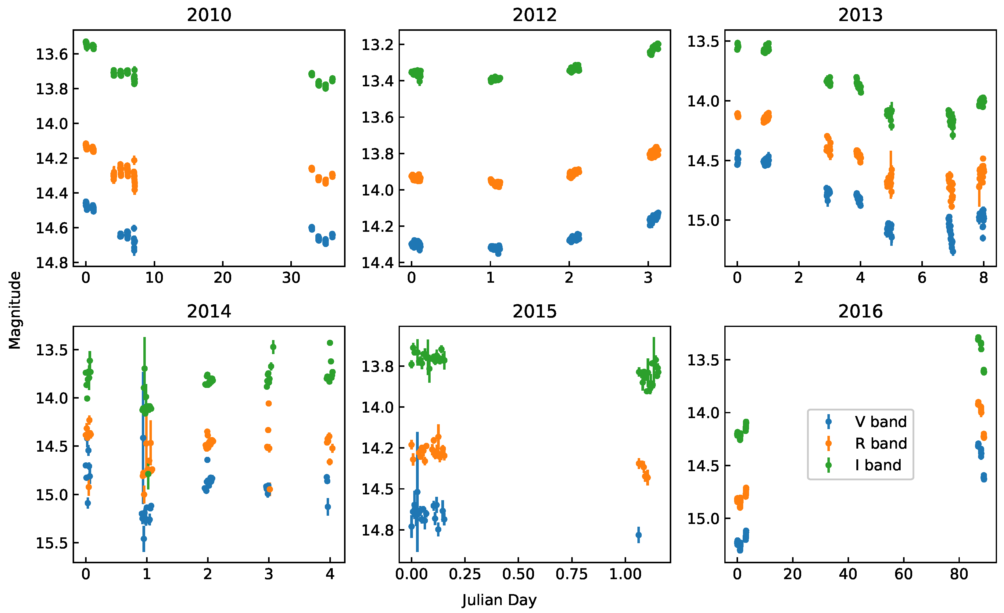
| Year | Nights | V(N) | R(N) | I(N) |
|---|---|---|---|---|
| 2010 | 10 | 183 | 196 | 197 |
| 2012 | 4 | 133 | 136 | 136 |
| 2013 | 7 | 142 | 153 | 156 |
| 2014 | 5 | 42 | 46 | 55 |
| 2015 | 2 | 19 | 25 | 39 |
| 2016 | 6 | 199 | 201 | 197 |
| Star | V | R | I |
|---|---|---|---|
| ID | (mag) | (mag) | (mag) |
| 4 | 14.18 (0.04) | 13.74 (0.04) | 13.28 (0.04) |
| 10 | 14.60 (0.05) | 14.34 (0.05) | 14.03 (0.05) |
| Date | Band | N | Magnitude (mag) | F-Test | -Test | Amp % | Flux mJy | % | State |
|---|---|---|---|---|---|---|---|---|---|
| , , , | , , | ||||||||
| 6 March 2010 | V | 33 | 14.468 ± 0.011 | 2.996, 1.858, 2.318, 3.092 | 219.915, 53.486, 62.487 | 4.480 | 6.172 ± 0.063 | 0.908 ± 0.001 | PV |
| R | 33 | 14.136 ± 0.009 | 1.790, 2.214, 2.318, 3.092 | 42.286, 53.486, 62.487 | 3.205 | 6.520 ± 0.054 | 0.000 ± 0.000 | PV | |
| I | 33 | 13.543 ± 0.010 | 2.039, 0.685, 2.318, 3.092 | 79.848, 53.486, 62.487 | 3.284 | 10.079 ± 0.088 | 0.444 ± 0.002 | PV | |
| 7 March 2010 | V | 25 | 14.485 ± 0.009 | 1.783, 1.285, 2.659, 3.735 | 144.765, 42.980, 51.179 | 3.372 | 6.075 ± 0.050 | 0.653 ± 0.001 | PV |
| R | 25 | 14.152 ± 0.007 | 0.798, 1.501, 2.659, 3.735 | 21.153, 42.980, 51.179 | 2.748 | 6.425 ± 0.039 | 0.000 ± 0.000 | NV | |
| I | 25 | 13.559 ± 0.005 | 0.709, 0.365, 2.659, 3.735 | 34.276, 42.980, 51.179 | 2.273 | 9.932 ± 0.050 | 0.000 ± 0.000 | NV | |
| 10 March 2010 | R | 12 | 14.301 ± 0.014 | 0.936, 0.502, 4.462, 7.761 | 3.314, 24.725, 31.264 | 4.001 | 5.600 ± 0.071 | 0.000 ± 0.000 | NV |
| I | 12 | 13.713 ± 0.009 | 1.427, 0.706, 4.462, 7.761 | 46.593, 24.725, 31.264 | 2.900 | 8.625 ± 0.069 | 0.562 ± 0.002 | PV | |
| 11 March 2010 | V | 20 | 14.643 ± 0.005 | 1.146, 0.579, 3.027, 4.474 | 23.267, 36.191, 43.820 | 1.568 | 5.254 ± 0.027 | 0.000 ± 0.000 | NV |
| R | 19 | 14.268 ± 0.020 | 7.582, 8.658, 3.128, 4.683 | 309.459, 34.805, 42.312 | 6.029 | 5.773 ± 0.105 | 1.740 ± 0.003 | V | |
| I | 20 | 13.712 ± 0.007 | 1.382, 1.689, 3.027, 4.474 | 17.720, 36.191, 43.820 | 2.597 | 8.634 ± 0.059 | 0.000 ± 0.000 | NV | |
| 12 March 2010 | V | 26 | 14.636 ± 0.009 | 2.454, 2.456, 2.604, 3.629 | 33.089, 44.314, 52.620 | 3.879 | 5.287 ± 0.046 | 0.376 ± 0.003 | NV |
| R | 26 | 14.263 ± 0.016 | 1.599, 3.275, 2.604, 3.629 | 128.718, 44.314, 52.620 | 5.727 | 5.799 ± 0.084 | 1.275 ± 0.002 | PV | |
| I | 26 | 13.704 ± 0.006 | 1.287, 1.618, 2.604, 3.629 | 39.641, 44.314, 52.620 | 1.709 | 8.690 ± 0.047 | 0.265 ± 0.002 | NV | |
| 13 March 2010 | V | 11 | 14.679 ± 0.030 | 1.028, 2.299, 4.849, 8.754 | 29.427, 23.209, 29.588 | 12.060 | 5.083 ± 0.144 | 2.381 ± 0.007 | PV |
| R | 13 | 14.308 ± 0.042 | 3.205, 6.351, 4.155, 7.005 | 121.479, 26.217, 32.909 | 15.897 | 5.566 ± 0.215 | 3.605 ± 0.008 | PV | |
| I | 13 | 13.744 ± 0.019 | 1.566, 3.960, 4.155, 7.005 | 63.668, 26.217, 32.909 | 7.597 | 8.382 ± 0.147 | 1.523 ± 0.004 | PV | |
| 8 April 2010 | V | 16 | 14.602 ± 0.004 | 0.781, 1.767, 3.522, 5.535 | 2.780, 30.578, 37.697 | 1.395 | 5.454 ± 0.020 | 0.000 ± 0.000 | NV |
| R | 16 | 14.261 ± 0.003 | 1.034, 0.769, 3.522, 5.535 | 3.770, 30.578, 37.697 | 1.015 | 5.807 ± 0.016 | 0.000 ± 0.000 | NV | |
| I | 16 | 13.717 ± 0.004 | 0.662, 1.544, 3.522, 5.535 | 30.781, 30.578, 37.697 | 1.199 | 8.587 ± 0.028 | 0.197 ± 0.001 | PV | |
| 9 April 2010 | V | 16 | 14.664 ± 0.007 | 1.056, 1.612, 3.522, 5.535 | 17.115, 30.578, 37.697 | 2.216 | 5.154 ± 0.031 | 0.000 ± 0.000 | NV |
| R | 16 | 14.317 ± 0.005 | 1.194, 1.316, 3.522, 5.535 | 11.264, 30.578, 37.697 | 1.662 | 5.517 ± 0.025 | 0.000 ± 0.000 | NV | |
| I | 16 | 13.772 ± 0.006 | 1.201, 3.118, 3.522, 5.535 | 39.401, 30.578, 37.697 | 2.344 | 8.165 ± 0.046 | 0.416 ± 0.001 | PV | |
| 10 April 2010 | V | 21 | 14.680 ± 0.008 | 0.991, 1.034, 2.938, 4.290 | 31.456, 37.566, 45.315 | 2.504 | 5.079 ± 0.038 | 0.000 ± 0.000 | NV |
| R | 21 | 14.333 ± 0.006 | 0.987, 1.140, 2.938, 4.290 | 19.336, 37.566, 45.315 | 2.162 | 5.434 ± 0.028 | 0.000 ± 0.000 | NV | |
| I | 21 | 13.786 ± 0.007 | 1.137, 1.657, 2.938, 4.290 | 30.316, 37.566, 45.315 | 2.185 | 8.060 ± 0.052 | 0.000 ± 0.000 | NV | |
| 11 April 2010 | V | 15 | 14.644 ± 0.007 | 0.816, 1.661, 3.698, 5.930 | 13.450, 29.141, 36.123 | 1.776 | 5.247 ± 0.031 | 0.000 ± 0.000 | NV |
| R | 15 | 14.297 ± 0.004 | 0.923, 0.620, 3.698, 5.930 | 8.547, 29.141, 36.123 | 1.651 | 5.620 ± 0.021 | 0.000 ± 0.000 | NV | |
| I | 15 | 13.749 ± 0.005 | 1.502, 0.635, 3.698, 5.930 | 18.913, 29.141, 36.123 | 1.653 | 8.341 ± 0.039 | 0.113 ± 0.004 | NV | |
| 12 April 2012 | V | 35 | 14.301 ± 0.011 | 0.867, 1.752, 2.258, 2.983 | 46.245, 56.061, 65.247 | 5.208 | 7.197 ± 0.075 | 0.000 ± 0.000 | NV |
| R | 36 | 13.936 ± 0.010 | 0.781, 1.054, 2.231, 2.934 | 49.662, 57.342, 66.619 | 3.440 | 7.834 ± 0.070 | 0.000 ± 0.000 | NV | |
| I | 37 | 13.358 ± 0.012 | 1.144, 0.759, 2.205, 2.888 | 64.849, 58.619, 67.985 | 5.876 | 11.959 ± 0.126 | 0.627 ± 0.002 | PV | |
| 13 April 2012 | V | 24 | 14.322 ± 0.010 | 0.830, 1.150, 2.719, 3.853 | 26.900, 41.638, 49.728 | 4.340 | 7.060 ± 0.063 | 0.000 ± 0.000 | NV |
| R | 25 | 13.964 ± 0.010 | 1.058, 2.296, 2.659, 3.735 | 38.305, 42.980, 51.179 | 4.025 | 7.636 ± 0.068 | 0.234 ± 0.005 | PV | |
| I | 25 | 13.389 ± 0.006 | 0.494, 0.577, 2.659, 3.735 | 28.780, 42.980, 51.179 | 2.775 | 11.616 ± 0.064 | 0.000 ± 0.000 | NV | |
| 14 April 2012 | V | 38 | 14.268 ± 0.010 | 0.925, 0.927, 2.181, 2.844 | 35.374, 59.893, 69.346 | 4.220 | 7.417 ± 0.068 | 0.000 ± 0.000 | PV |
| R | 39 | 13.906 ± 0.010 | 1.039, 0.903, 2.157, 2.803 | 58.151, 61.162, 70.703 | 4.463 | 8.054 ± 0.077 | 0.000 ± 0.000 | NV | |
| I | 39 | 13.333 ± 0.010 | 0.938, 1.674, 2.157, 2.803 | 96.397, 61.162, 70.703 | 3.846 | 12.235 ± 0.113 | 0.658 ± 0.001 | PV | |
| 15 April 2012 | V | 36 | 14.157 ± 0.016 | 0.763, 1.056, 2.231, 2.934 | 114.645, 57.342, 66.619 | 6.646 | 8.219 ± 0.117 | 0.650 ± 0.004 | PV |
| R | 36 | 13.795 ± 0.016 | 1.698, 1.443, 2.231, 2.934 | 123.812, 57.342, 66.619 | 5.563 | 8.922 ± 0.130 | 1.025 ± 0.002 | PV | |
| I | 35 | 13.224 ± 0.015 | 1.085, 1.146, 2.258, 2.983 | 150.305, 56.061, 65.247 | 5.932 | 13.528 ± 0.186 | 1.048 ± 0.002 | PV | |
| 16 March 2013 | V | 9 | 14.484 ± 0.038 | 2.330, 0.912, 6.029, 12.046 | 29.022, 20.090, 26.124 | 9.137 | 6.085 ± 0.213 | 2.830 ± 0.010 | PV |
| R | 9 | 14.119 ± 0.010 | 0.116, 0.919, 6.029, 12.046 | 3.322, 20.090, 26.124 | 2.837 | 6.620 ± 0.064 | 0.000 ± 0.000 | NV | |
| I | 9 | 13.546 ± 0.018 | 0.488, 1.091, 6.029, 12.046 | 27.032, 20.090, 26.124 | 5.120 | 10.056 ± 0.165 | 0.877 ± 0.007 | PV | |
| 17 March 2013 | V | 27 | 14.509 ± 0.018 | 0.584, 1.063, 2.554, 3.532 | 34.531, 45.642, 54.052 | 7.448 | 5.942 ± 0.096 | 0.000 ± 0.000 | NV |
| R | 29 | 14.149 ± 0.019 | 1.534, 2.097, 2.464, 3.362 | 63.400, 48.278, 56.892 | 7.599 | 6.444 ± 0.112 | 0.882 ± 0.005 | PV | |
| I | 29 | 13.569 ± 0.018 | 0.474, 1.714, 2.464, 3.362 | 71.269, 48.278, 56.892 | 7.763 | 9.843 ± 0.160 | 1.176 ± 0.003 | PV | |
| 19 March 2013 | V | 14 | 14.771 ± 0.027 | 0.877, 1.384, 3.905, 6.409 | 15.011, 27.688, 34.528 | 9.850 | 4.669 ± 0.114 | 1.090 ± 0.010 | NV |
| R | 17 | 14.395 ± 0.039 | 2.594, 4.396, 3.372, 5.205 | 74.936, 32.000, 39.252 | 15.179 | 5.138 ± 0.189 | 3.168 ± 0.007 | PV | |
| I | 17 | 13.837 ± 0.017 | 0.762, 0.926, 3.372, 5.205 | 31.938, 32.000, 39.252 | 6.710 | 7.691 ± 0.124 | 0.801 ± 0.006 | NV | |
| 20 March 2013 | V | 22 | 14.820 ± 0.026 | 2.317, 2.289, 2.857, 4.127 | 57.574, 38.932, 46.797 | 9.760 | 4.464 ± 0.108 | 1.803 ± 0.005 | PV |
| R | 23 | 14.454 ± 0.024 | 4.800, 3.911, 2.785, 3.983 | 57.654, 40.289, 48.268 | 9.423 | 4.863 ± 0.106 | 1.564 ± 0.004 | V | |
| I | 24 | 13.871 ± 0.028 | 2.890, 3.196, 2.719, 3.853 | 189.788, 41.638, 49.728 | 12.291 | 7.458 ± 0.191 | 2.310 ± 0.004 | PV | |
| 21 March 2013 | V | 24 | 15.074 ± 0.031 | 1.165, 0.624, 2.719, 3.853 | 38.513, 41.638, 49.728 | 11.054 | 3.533 ± 0.101 | 1.050 ± 0.011 | NV |
| R | 26 | 14.680 ± 0.038 | 1.070, 0.460, 2.604, 3.629 | 64.444, 44.314, 52.620 | 17.809 | 3.951 ± 0.140 | 0.000 ± 0.000 | PV | |
| I | 26 | 14.103 ± 0.028 | 1.161, 0.612, 2.604, 3.629 | 32.312, 44.314, 52.620 | 12.661 | 6.022 ± 0.148 | 0.958 ± 0.009 | NV | |
| 23 March 2013 | V | 18 | 15.102 ± 0.086 | 4.072, 4.066, 3.242, 4.924 | 155.018, 33.409, 40.790 | 26.438 | 3.451 ± 0.271 | 7.236 ± 0.014 | V |
| R | 21 | 14.716 ± 0.077 | 4.759, 4.914, 2.938, 4.290 | 197.476, 37.566, 45.315 | 24.118 | 3.831 ± 0.265 | 6.347 ± 0.012 | V | |
| I | 23 | 14.153 ± 0.048 | 1.671, 1.774, 2.785, 3.983 | 112.549, 40.289, 48.268 | 19.815 | 5.755 ± 0.250 | 3.583 ± 0.008 | PV | |
| 24 March 2013 | V | 28 | 14.981 ± 0.045 | 3.927, 3.201, 2.507, 3.443 | 97.643, 46.963, 55.476 | 22.681 | 3.851 ± 0.153 | 3.383 ± 0.006 | V |
| R | 28 | 14.598 ± 0.048 | 0.224, 1.097, 2.507, 3.443 | 116.079, 46.963, 55.476 | 22.819 | 4.262 ± 0.185 | 2.327 ± 0.011 | PV | |
| I | 28 | 14.012 ± 0.022 | 1.513, 2.013, 2.507, 3.443 | 103.345, 46.963, 55.476 | 7.233 | 6.547 ± 0.136 | 1.623 ± 0.004 | PV | |
| 31 March 2014 | V | 7 | 14.729 ± 0.199 | 4.712, 8.024, 8.466, 20.030 | 81.483, 16.812, 22.458 | 60.883 | 4.936 ± 0.891 | 17.063 ± 0.051 | PV |
| R | 7 | 14.430 ± 0.209 | 56.965, 52.442, 8.466, 20.030 | 72.512, 16.812, 22.458 | 62.691 | 5.053 ± 0.824 | 15.795 ± 0.045 | V | |
| I | 8 | 13.786 ± 0.108 | 1.572, 0.982, 6.993, 15.019 | 297.725, 18.475, 24.322 | 36.097 | 8.102 ± 0.785 | 7.760 ± 0.030 | PV | |
| 1 April 2014 | V | 12 | 15.164 ± 0.242 | 0.029, 1.201, 4.462, 7.761 | 34.159, 24.725, 31.264 | 98.843 | 3.347 ± 0.974 | 0.000 ± 0.000 | PV |
| R | 11 | 14.725 ± 0.144 | 0.091, 1.260, 4.849, 8.754 | 87.322, 23.209, 29.588 | 49.352 | 3.824 ± 0.521 | 2.436 ± 0.163 | PV | |
| I | 13 | 14.105 ± 0.231 | 0.717, 2.427, 4.155, 7.005 | 166.964, 26.217, 32.909 | 104.231 | 6.133 ± 1.159 | 13.975 ± 0.050 | PV | |
| 2 April 2014 | V | 15 | 14.869 ± 0.074 | 11.715, 10.409, 3.698, 5.930 | 324.871, 29.141, 36.123 | 30.330 | 4.277 ± 0.310 | 6.913 ± 0.014 | V |
| R | 15 | 14.458 ± 0.045 | 10.458, 10.827, 3.698, 5.930 | 204.227, 29.141, 36.123 | 16.505 | 4.849 ± 0.205 | 3.999 ± 0.008 | V | |
| I | 15 | 13.826 ± 0.033 | 3.458, 2.949, 3.698, 5.930 | 291.375, 29.141, 36.123 | 9.400 | 7.772 ± 0.238 | 2.869 ± 0.006 | PV | |
| 3 April 2014 | V | 4 | 14.941 ± 0.033 | 0.625, 1.733, 29.457, 141.108 | 5.923, 11.345, 16.266 | 7.140 | 3.994 ± 0.121 | 1.760 ± 0.018 | NV |
| R | 6 | 14.481 ± 0.265 | 59.894, 73.206, 10.967, 29.752 | 1001.118, 15.086, 20.515 | 80.609 | 4.884 ± 1.174 | 23.894 ± 0.070 | V | |
| I | 8 | 13.750 ± 0.121 | 8.107, 3.941, 6.993, 15.019 | 443.834, 18.475, 24.322 | 37.464 | 8.385 ± 1.006 | 11.503 ± 0.031 | PV | |
| 4 April 2014 | V | 4 | 14.958 ± 0.124 | 6.919, 2.946, 29.457, 141.108 | 50.771, 11.345, 16.266 | 25.301 | 3.954 ± 0.443 | 10.089 ± 0.044 | PV |
| R | 7 | 14.478 ± 0.084 | 2.329, 4.181, 8.466, 20.030 | 49.708, 16.812, 22.458 | 23.629 | 4.772 ± 0.350 | 6.598 ± 0.022 | PV | |
| I | 11 | 13.701 ± 0.155 | 101.854, 98.563, 4.849, 8.754 | 1163.937, 23.209, 29.588 | 42.137 | 8.815 ± 1.379 | 15.563 ± 0.034 | V | |
| 27 March 2015 | V | 17 | 14.650 ± 0.053 | 0.129, 0.562, 3.372, 5.205 | 18.000, 32.000, 39.252 | 21.636 | 5.228 ± 0.258 | 0.000 ± 0.000 | NV |
| R | 17 | 14.270 ± 0.039 | 0.431, 1.543, 3.372, 5.205 | 35.530, 32.000, 39.252 | 13.775 | 5.766 ± 0.210 | 1.923 ± 0.012 | PV | |
| I | 21 | 13.699 ± 0.030 | 0.401, 0.751, 2.938, 4.290 | 23.917, 37.566, 45.315 | 12.073 | 8.736 ± 0.242 | 0.000 ± 0.000 | NV | |
| 28 March 2015 | V | 2 | 14.715 ± 0.068 | — | — | 9.546 | 4.928 ± 0.306 | 3.685 ± 0.052 | — |
| R | 8 | 14.384 ± 0.034 | 0.439, 0.354, 6.993, 15.019 | 10.458, 18.475, 24.322 | 7.135 | 5.187 ± 0.162 | 0.000 ± 0.000 | NV | |
| I | 18 | 13.802 ± 0.053 | 0.800, 0.458, 3.242, 4.924 | 95.727, 33.409, 40.790 | 17.694 | 7.954 ± 0.384 | 0.970 ± 0.040 | PV | |
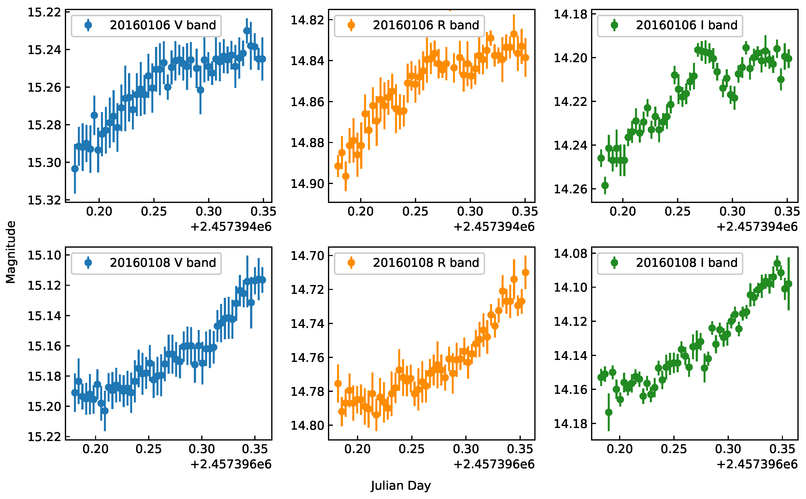
| 5 January 2016 | V | 49 | 15.233 ± 0.009 | 3.775, 5.041, 1.977, 2.489 | 39.766, 73.683, 84.037 | 4.124 | 3.052 ± 0.024 | 0.000 ± 0.000 | PV |
| R | 49 | 14.830 ± 0.009 | 3.676, 3.784, 1.977, 2.489 | 104.805, 73.683, 84.037 | 3.368 | 3.441 ± 0.029 | 0.527 ± 0.001 | V | |
| I | 49 | 14.201 ± 0.007 | 1.467, 1.474, 1.977, 2.489 | 109.280, 73.683, 84.037 | 3.264 | 5.500 ± 0.034 | 0.413 ± 0.001 | PV | |
| 6 January 2016 | V | 50 | 15.260 ± 0.018 | 11.933, 15.218, 1.963, 2.465 | 165.498, 74.919, 85.351 | 6.872 | 2.975 ± 0.050 | 1.346 ± 0.002 | V |
| R | 50 | 14.852 ± 0.020 | 17.948, 18.593, 1.963, 2.465 | 395.483, 74.919, 85.351 | 8.972 | 3.371 ± 0.061 | 1.635 ± 0.002 | V | |
| I | 50 | 14.218 ± 0.018 | 8.024, 10.653, 1.963, 2.465 | 771.064, 74.919, 85.351 | 5.789 | 5.417 ± 0.087 | 1.547 ± 0.002 | V | |
| 8 January 2016 | V | 52 | 15.167 ± 0.024 | 37.909, 37.202, 1.936, 2.419 | 251.989, 77.386, 87.968 | 7.998 | 3.243 ± 0.073 | 1.956 ± 0.003 | V |
| R | 51 | 14.764 ± 0.022 | 25.587, 28.567, 1.949, 2.441 | 340.977, 76.154, 86.661 | 7.788 | 3.655 ± 0.076 | 1.870 ± 0.002 | V | |
| I | 51 | 14.134 ± 0.023 | 9.004, 10.514, 1.949, 2.441 | 1089.284, 76.154, 86.661 | 8.108 | 5.852 ± 0.126 | 2.084 ± 0.002 | V | |
| 1 April 2016 | V | 12 | 14.305 ± 0.007 | 1.185, 0.758, 4.462, 7.761 | 7.032, 24.725, 31.264 | 2.439 | 7.171 ± 0.048 | 0.000 ± 0.000 | NV |
| R | 12 | 13.912 ± 0.007 | 1.625, 1.915, 4.462, 7.761 | 11.356, 24.725, 31.264 | 2.190 | 8.010 ± 0.051 | 0.000 ± 0.000 | NV | |
| I | 11 | 13.297 ± 0.007 | 3.768, 4.057, 4.849, 8.754 | 231.306, 23.209, 29.588 | 2.148 | 12.651 ± 0.078 | 0.577 ± 0.001 | PV | |
| 2 April 2016 | V | 10 | 14.364 ± 0.024 | 1.266, 2.796, 5.351, 10.107 | 93.338, 21.666, 27.877 | 6.432 | 6.793 ± 0.151 | 1.516 ± 0.007 | PV |
| R | 10 | 13.969 ± 0.021 | 1.404, 0.485, 5.351, 10.107 | 192.535, 21.666, 27.877 | 4.774 | 7.604 ± 0.145 | 0.602 ± 0.013 | PV | |
| I | 7 | 13.353 ± 0.020 | 0.863, 2.103, 8.466, 20.030 | 84.205, 16.812, 22.458 | 5.465 | 12.017 ± 0.217 | 1.561 ± 0.006 | PV | |
| 3 April 2016 | V | 26 | 14.616 ± 0.009 | 0.253, 1.588, 2.604, 3.629 | 32.455, 44.314, 52.620 | 3.759 | 5.385 ± 0.043 | 0.000 ± 0.000 | NV |
| R | 29 | 14.226 ± 0.008 | 0.412, 1.525, 2.464, 3.362 | 42.732, 48.278, 56.892 | 3.556 | 5.997 ± 0.047 | 0.246 ± 0.003 | NV | |
| I | 29 | 13.609 ± 0.006 | 0.517, 0.920, 2.464, 3.362 | 80.325, 48.278, 56.892 | 2.370 | 9.491 ± 0.049 | 0.239 ± 0.001 | PV |
| Date | Band | ID | ||||
|---|---|---|---|---|---|---|
| +2,456,000 | min | min | ||||
| 17 March 2013 | R | 1 | 0.192 ± 0.052 | 369.037 | 10.612 ± 4.861 | 7.916 ± 3.970 |
| 2 | 0.291 ± 0.048 | 369.104 | 15.788 ± 3.865 | 5.326 ± 1.983 | ||
| 3 | 0.342 ± 0.049 | 369.164 | 13.585 ± 3.228 | 9.547 ± 3.588 | ||
| 20 March 2013 | V | 1 | 0.159 ± 0.061 | 372.136 ± 0.002 | 21.615 ± 12.064 | 2.712 ± 4.668 |
| 5 January 2016 | V | 1 | 0.063 ± 0.009 | 1393.282 ± 0.007 | 14.594 ± 6.451 | 19.763 ± 7.906 |
| R | 1 | 0.052 ± 0.014 | 1393.275 ± 0.006 | 9.160 ± 6.090 | 36.480 ± 16.328 | |
| I | 1 | 0.056 ± 0.015 | 1393.274 ± 0.004 | 6.536 ± 4.596 | 44.752 ± 17.941 | |
| 6 January 2016 | I | 1 | 0.079 ± 0.016 | 1394.282 ± 0.003 | 37.986 ± 14.515 | 4.672 ± 2.890 |
| Date | Data Points | Slope | Intercept | Pearson’s Coefficient | Pro |
|---|---|---|---|---|---|
| 6 March 2010 | 49 | −0.460 ± 0.188 | 6.833 ± 2.661 | −0.336 | 0.018 |
| 7 March 2010 | 22 | −0.145 ± 0.235 | 2.382 ± 3.324 | −0.137 | 0.545 |
| 11 March 2010 | 22 | −0.954 ± 0.063 | 13.989 ± 0.895 | −0.959 | 0.000 |
| 12 March 2010 | 35 | −0.935 ± 0.108 | 13.702 ± 1.539 | −0.833 | 0.000 |
| 8 April 2010 | 16 | −0.311 ± 0.295 | 4.774 ± 4.210 | −0.271 | 0.310 |
| 9 April 2010 | 16 | −0.671 ± 0.346 | 9.950 ± 4.951 | −0.460 | 0.073 |
| 10 April 2010 | 40 | −1.026 ± 0.245 | 15.047 ± 3.506 | −0.562 | 0.000 |
| 11 April 2010 | 29 | −0.783 ± 0.292 | 11.547 ± 4.171 | −0.459 | 0.012 |
| 12 April 2012 | 69 | −0.918 ± 0.147 | 13.157 ± 2.053 | −0.606 | 0.000 |
| 13 April 2012 | 24 | −1.151 ± 0.209 | 16.434 ± 2.917 | −0.762 | 0.000 |
| 14 April 2012 | 75 | −0.623 ± 0.106 | 9.033 ± 1.473 | −0.567 | 0.000 |
| 15 April 2012 | 71 | −0.541 ± 0.104 | 7.827 ± 1.440 | −0.529 | 0.000 |
| 17 March 2013 | 27 | −0.730 ± 0.179 | 10.689 ± 2.528 | −0.633 | 0.000 |
| 20 March 2013 | 21 | −0.419 ± 0.182 | 6.421 ± 2.626 | −0.468 | 0.033 |
| 21 March 2013 | 24 | −0.891 ± 0.179 | 13.471 ± 2.628 | −0.728 | 0.000 |
| 27 March 2015 | 14 | −1.225 ± 0.293 | 17.866 ± 4.182 | −0.770 | 0.001 |
| 5 January 2016 | 49 | −0.296 ± 0.095 | 4.795 ± 1.411 | −0.413 | 0.003 |
| 6 January 2016 | 50 | −0.157 ± 0.056 | 2.742 ± 0.839 | −0.373 | 0.008 |
| 8 January 2016 | 51 | 0.011 ± 0.041 | 0.234 ± 0.600 | 0.040 | 0.778 |
| 3 April 2016 | 25 | −0.161 ± 0.117 | 2.679 ± 1.659 | −0.276 | 0.181 |
© 2017 by the authors. Licensee MDPI, Basel, Switzerland. This article is an open access article distributed under the terms and conditions of the Creative Commons Attribution (CC BY) license (http://creativecommons.org/licenses/by/4.0/).
Share and Cite
Zeng, W.; Zhao, Q.-J.; Jiang, Z.-J.; Kong, Z.-H.; Liu, Z.; Wang, D.-D.; Geng, X.-F.; Yang, S.-B.; Dai, B.-Z. Intra-Night Variability of OJ 287 with Long-Term Multiband Optical Monitoring. Galaxies 2017, 5, 85. https://doi.org/10.3390/galaxies5040085
Zeng W, Zhao Q-J, Jiang Z-J, Kong Z-H, Liu Z, Wang D-D, Geng X-F, Yang S-B, Dai B-Z. Intra-Night Variability of OJ 287 with Long-Term Multiband Optical Monitoring. Galaxies. 2017; 5(4):85. https://doi.org/10.3390/galaxies5040085
Chicago/Turabian StyleZeng, Wei, Qing-Jiang Zhao, Ze-Jun Jiang, Zhi-Hui Kong, Zhen Liu, Dong-Dong Wang, Xiong-Fei Geng, Shen-Bang Yang, and Ben-Zhong Dai. 2017. "Intra-Night Variability of OJ 287 with Long-Term Multiband Optical Monitoring" Galaxies 5, no. 4: 85. https://doi.org/10.3390/galaxies5040085