An Overview of X-Ray Polarimetry of Astronomical Sources

NASA/Marshall Space Flight Center (MSFC), ST12, 320 Sparkman Drive, Huntsville, AL 35805, USA
Galaxies 2018, 6(1), 33; https://doi.org/10.3390/galaxies6010033
Submission received: 19 January 2018
/
Revised: 26 February 2018
/
Accepted: 1 March 2018
/
Published: 6 March 2018
(This article belongs to the Special Issue The Bright Future of Astronomical X-ray Polarimetry)
Abstract
:We review the history of astronomical X-ray polarimetry based on the author’s perspective, beginning with early sounding-rocket experiments by Robert Novick at Columbia University and his team, of which the author was a member. After describing various early techniques for measuring X-ray polarization, we discuss the polarimeter aboard the Orbiting Solar Observatory 8 (OSO-8) and its scientific results. Next, we describe the X-ray polarimeter to have flown aboard the ill-fated original Spectrum-X mission, which provided important lessons on polarimeter design, systematic effects, and the programmatics of a shared focal plane. We conclude with a description of the Imaging X-ray Polarimetry Explorer (IXPE) and its prospective scientific return. IXPE, a partnership between NASA and ASI, has been selected as a NASA Astrophysics Small Explorers Mission and is currently scheduled to launch in April of 2021.
1. Introduction
Polarization measurements uniquely probe physical anisotropies—ordered magnetic fields, aspheric matter distributions, and general relativistic coupling to black-hole spin. Polarization measurements in X-ray astronomy add an important, and relatively unexplored, dimension to the parameter space for investigating cosmic X-ray sources and processes and for using extreme astrophysical environments as laboratories for fundamental physics. Specifically, the degree of polarization and the position angle of the electric vector on the sky depend on the conditions under which the X-rays are produced. Therefore, modelling of the physical processes and the geometry must be consistent with the observed polarization
Despite this, only a few experiments have conducted unambiguous measurements of the linear polarization of sources of X-rays. We review the history of X-ray polarimetry, concentrating primarily on the author’s direct participation in such ventures, and describe the results and the experimental techniques. We conclude with a brief description of the Imaging X-ray Polarimetry Explorer (IXPE), a joint venture involving NASA and the Italian Space Agency (ASI), to be launched as a NASA Small Explorer mission in early 2021.
2. Background—Prior to IXPE
2.1. The First Sounding Rocket Experiments
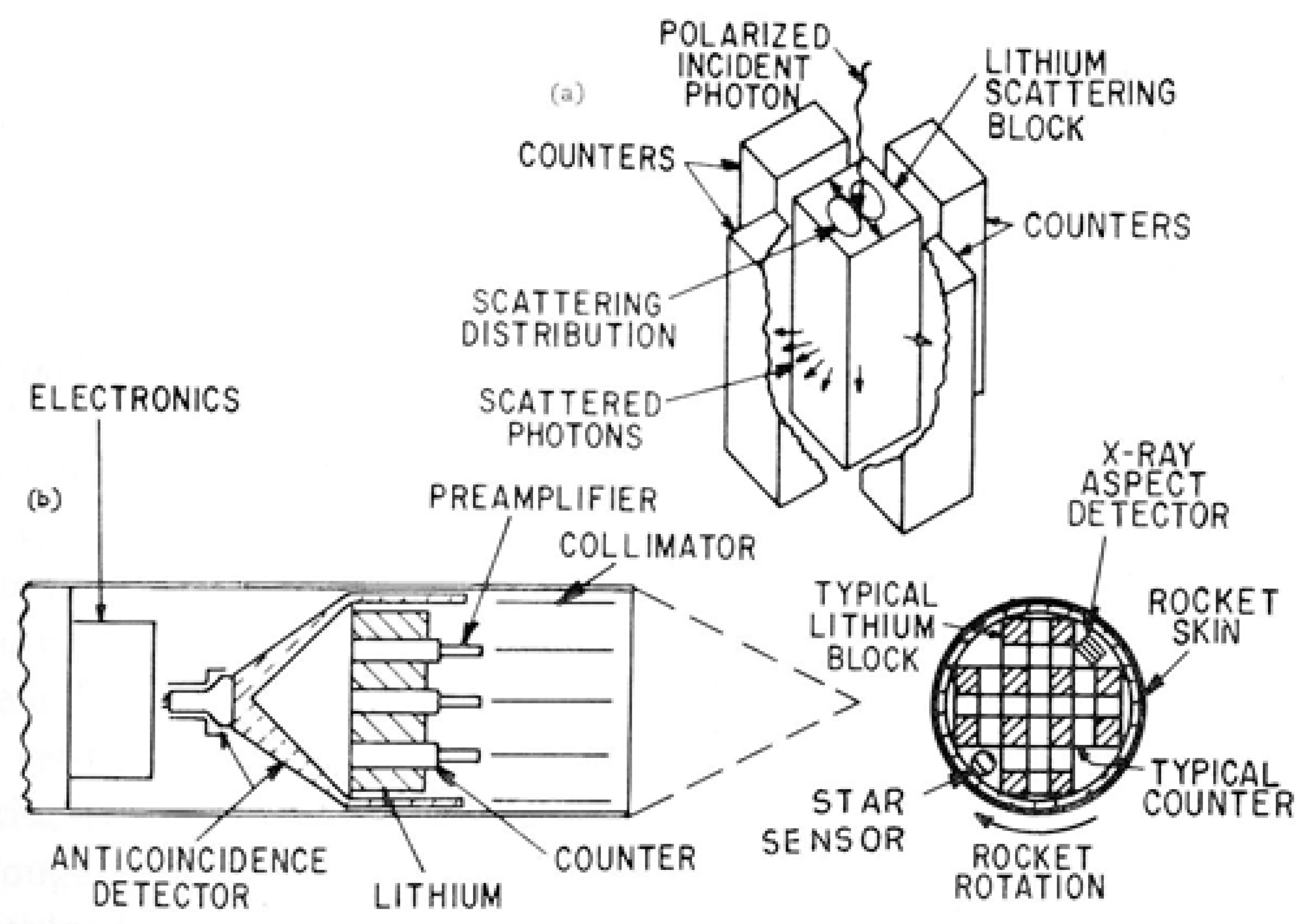
The first sounding rocket flown in an attempt to measure the linear polarization of a non-solar source of X-rays was launched in July of 1968 by the group at Columbia University under the direction of Professor Robert Novick. The target was Sco X-1. A schematic of the payload is shown in Figure 1. The polarimeter exploited the polarization dependence of Compton scattering using lithium as a scattering material. The payload was rotated around the line of sight to mitigate systematic effects, e.g., those imposed by the geometry.
There are a number of considerations involved in the design of the scattering polarimeter and these considerations, by and large, apply to all X-ray polarimeters. Of course the primary consideration is to achieve high sensitivity to a polarized signal. We introduced the concept of the minimum detectable polarization (MDP) at the 99% confidence level as the parameter to consider:
MDP99(%) = [4.29 × 10⁴/M(%)] × [(Rs + RB)/(RS2 × t)]1/2
The MDP is the degree of polarization detected at the 99% confidence level independent of the position angle. M is the variation in the signal as a function of the azimuthal angle produced in the instrument by a 100% polarized signal with RB = 0, where RB is the background counting rate. RS is the source counting rate, and t is the integration time.
The lithium scattering polarimeter is often referred to as a Thomson scattering polarimeter, because the Thomsom cross-section:
provides a fairly accurate approximation to the angular dependence of the scattered photon. Here theta is the polar scattering angle and phi is the azimuthal angle measured from the initial polarization direction. Of course, for bound electrons, one must account for both coherent and incoherent scattering and, for this experiment, photoelectric absorption:
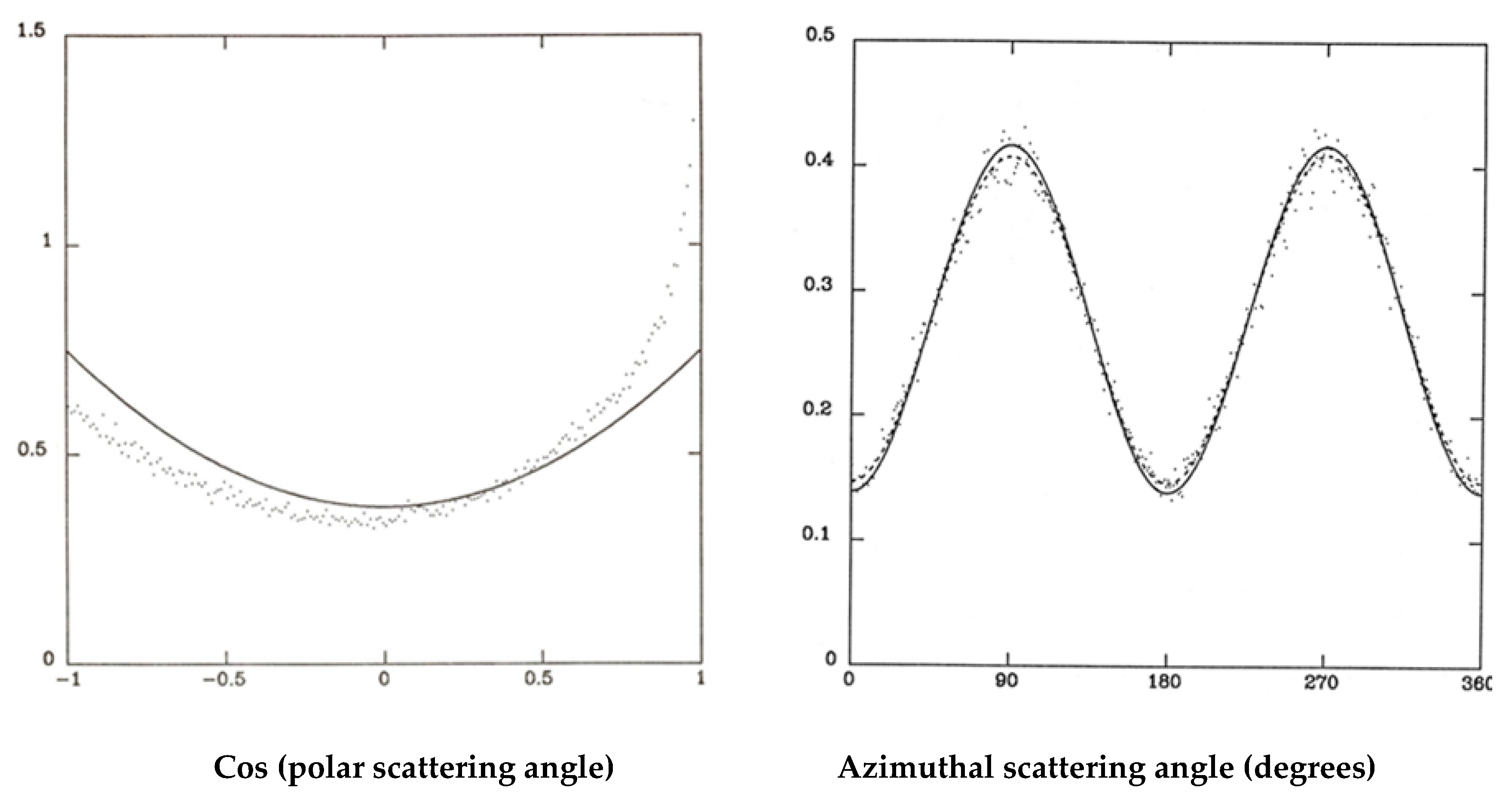
Here, F and I are the relevant atomic scattering factors and are, themselves, functions of sin(θ/2)/λ. Figure 2 compares the Thomson approximation to actual angular distributions.
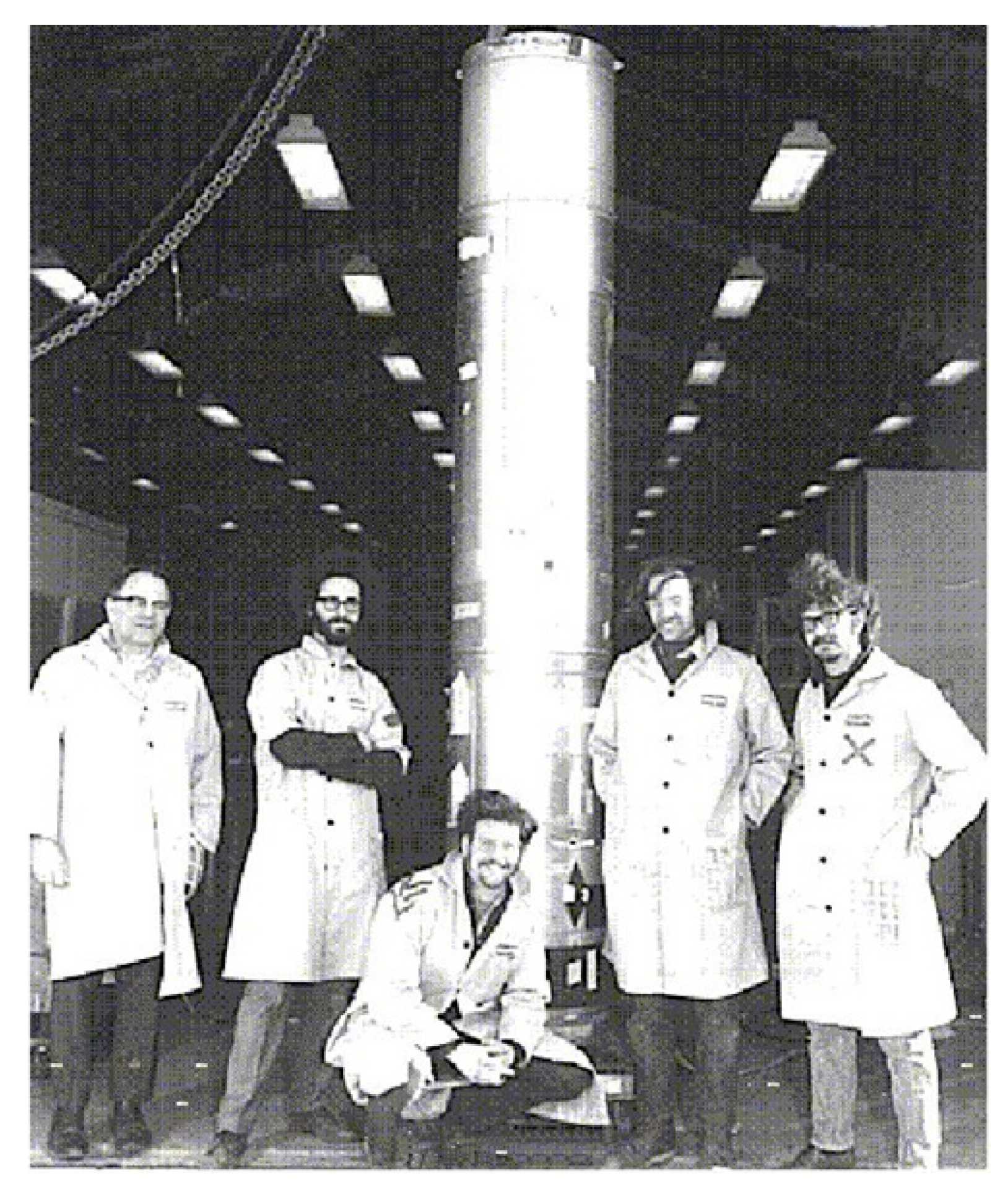
This first sounding rocket flight made no detection, providing an upper limit of the order of 20% to the degree of polarization. One needed detectors more sensitive to polarization, especially within the observing time limitations of a sounding rocket flight. This led the group to consider Bragg reflection from crystals set at 45 degrees with respect to the incident beam [1]. Bragg crystals are inherently narrow-band devices and, so, the limited throughput might at first be considered as an obstacle to the advantages provided by a polarimeter with a 100% modulation factor. There are, as we learned, ideally imperfect or mosaic crystals that optimize the throughput. The next rocket polarimeter, which included mosaic graphite crystal polarimeters sensitive in the first-order at 2.6 keV, is schematically shown in Figure 3. Figure 4 is a photograph of the payload and the individuals involved with its success.
The flight was quite successful, despite the fact that one of the doors did not open and the payload sank into the water off the coast of Wallops Island, and so the film-bearing aspect camera could not be recovered. The target was the Crab Nebula and its pulsar and the experiment provided the first detection of the X-ray polarization from this system [2], confirming the synchrotron origin of the X-rays. Combining the data from both types of polarimeters led to a result of p = 15 ± 5% at a position angle of 156 ± 10° measured east of north.
2.2. The OSO-8 Polarimeter
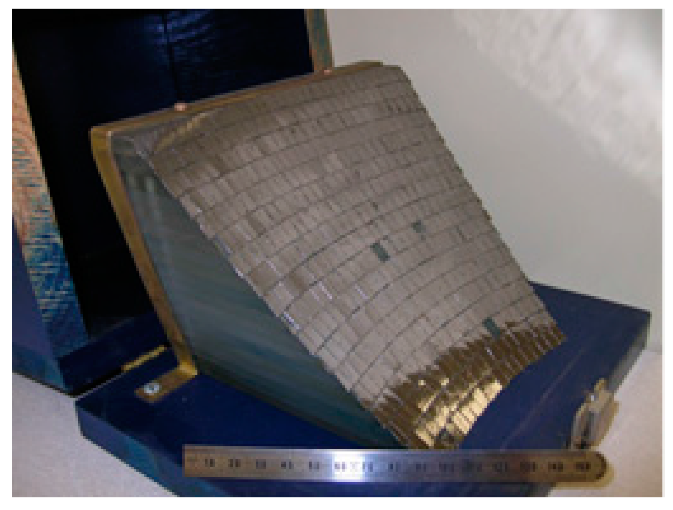
The next major step forward for X-ray polarimetry was the inclusion of two graphite crystal polarimeters aboard the Orbiting Solar Observatory (OSO-8) [3]. Figure 5 is a photograph of the engineering model of one of the crystal panels. Observation of the Crab, with the contamination of the pulsar removed, yielded a highly significant measurement of p = 19 ± 1% at a position angle of 156.4 ± 1.4° [4] measured east of north, satisfyingly in agreement with the previous measurement and leaving no doubt as to the synchrotron origin of the X-rays.
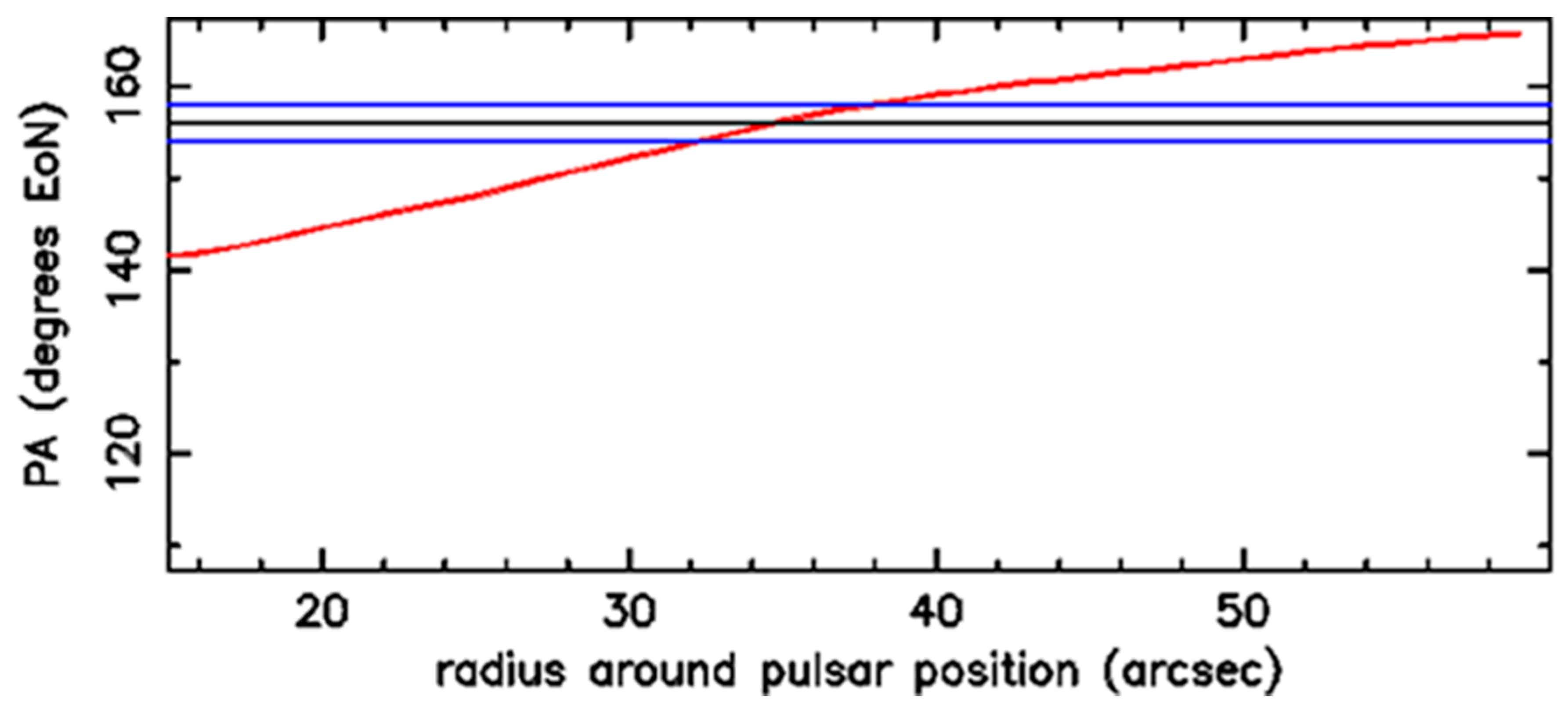
More recently we were able to check the likelihood that the X-ray measurements of the position angle were on track by calculating the average optical position angle from recent measurements with the Hubble Space Telescope (HST) [5] as a function of the radius of the region surrounding the pulsar. The results are shown in Figure 6 and the mean optical position angle is consistent with the OSO-8 X-ray measurements when the nebular size is in the range of 32–38 arcseconds, in excellent agreement with the size observed with the Chandra X-ray Observatory [6].
The OSO-8 satellite featured a number of different instruments, many with different viewing directions. This naturally resulted in an observing program where no one received the amount of observing time that they fully desired. This is generally a problem for instruments that are on an observatory that require long integration times to achieve their objectives, such as spectroscopy or polarimetry. In these cases the signal that one wishes to measure is typically a small fraction of the total flux, even ignoring the background. The limited number of experiments performed with the OSO-8 polarimeter, in general, yielded upper limits (e.g., [7,8]) with the exception of very marginal detections of polarization from Cygnus X-2 [9] and Cygnus X-1 [10].
2.3. The Stellar X-Ray Polarimeter
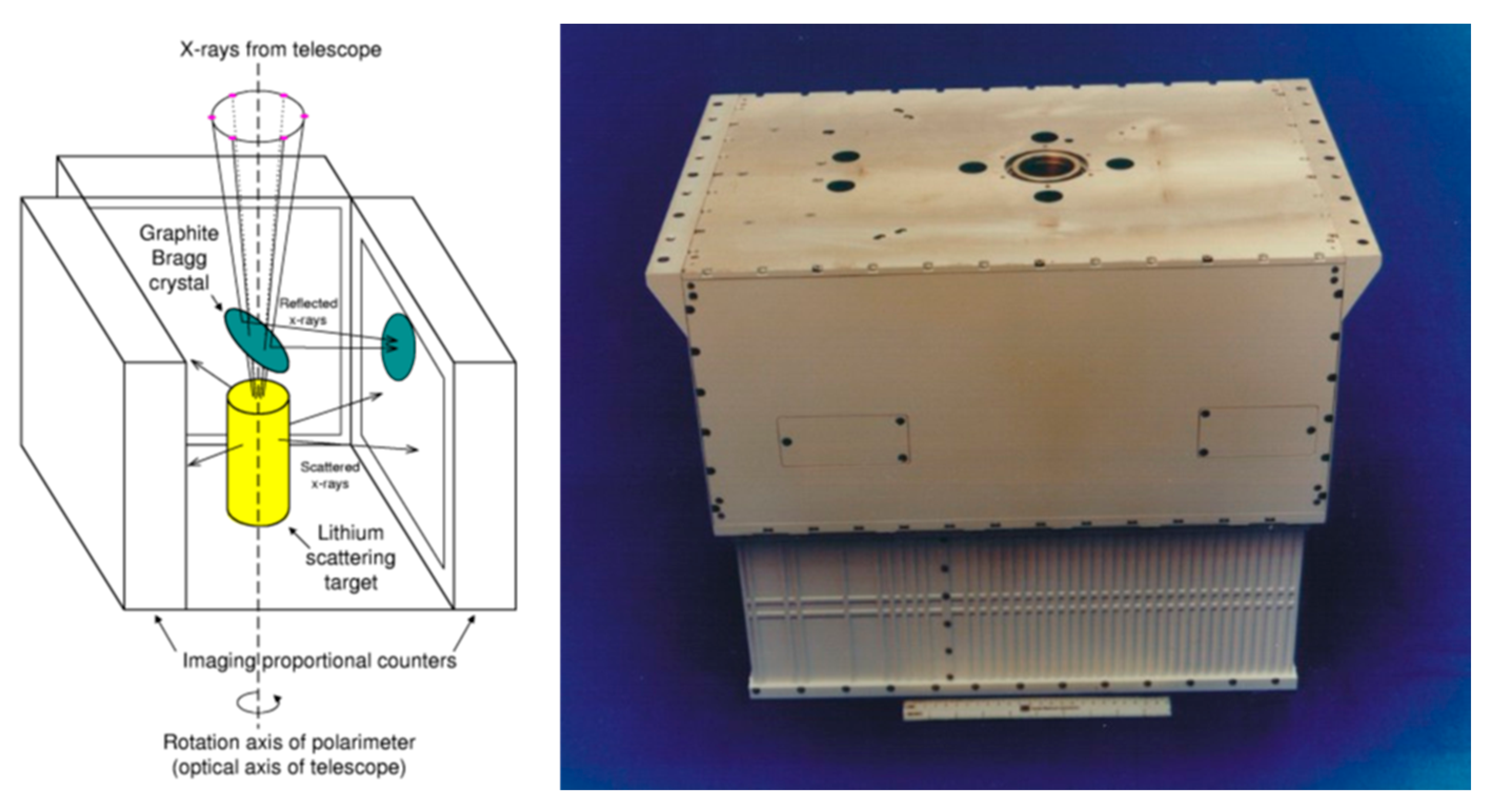
The next major step for X-ray polarimetry was the advent of the Stellar X-ray Polarimeter (SXRP). Funded by NASA and Italy, this instrument was designed to fly on the Russian mission Spectrum Roentgen-Gamma. The polarimeter was to be mounted on a slide and, occasionally, placed at the focus of a Danish foil X-ray telescope. The left-hand side of Figure 7 is a schematic of SXRP and the right-hand side is a photograph of the completed device. The device has been described in a number of publications (e.g., [11,12]).
Unfortunately the collapse of the Soviet Union in 1989 lead to the cancellation of the mission. SXRP also would have potentially suffered from being placed on an observatory—only 11 days of observing were assigned to SXRP for the first year of operation. We should also mention, for potential future renditions of this design, a systematic effect arises when placing a scattering polarimeter at the focus of an X-ray telescope [13].
2.4. Electron Tracking
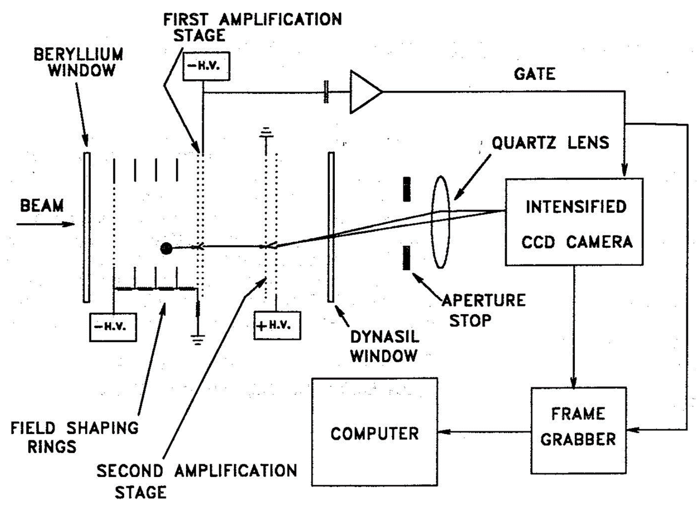
The next step in the development of detectors for X-ray polarimetry was based on the realization that the polarimeter must be capable of imaging because a large subset of astronomical X-ray sources, such as supernova remnants, are extended. Moreover, as noted in the case of SXRP, many of polarimeters are prone to systematic effects which would necessarily complicate the data analysis and, possibly, the interpretation of the results. In the early 1990s, Austin and Ramsey [14] demonstrated an optical imaging chamber for measuring the details of the tracks produced by the photoelectron in the gas of a proportional counter. Since the direction of the primary photoelectron released in the photoelectric absorption of the incident photon depends on the polarization of the incident beam, imaging the track provides information as to the degree of polarization and the position angle of the incident flux. To the extent that the detector pixels were extremely small compared to other characteristic lengths, this detector was devoid of systematic effects. A schematic of the device is shown in Figure 8 and an image of an electron track is shown in Figure 9. The track in Figure 9 emphasizes the importance of the track-recognition algorithms as the majority of charge appears at the end of the track where it has lost all sense of the initial direction of the primary photoelectron. Another obvious advantage of this device for imaging, at least over an imaging proportional counter, is the higher precision associated with the detection of the position of the initial interaction.
3. IXPE
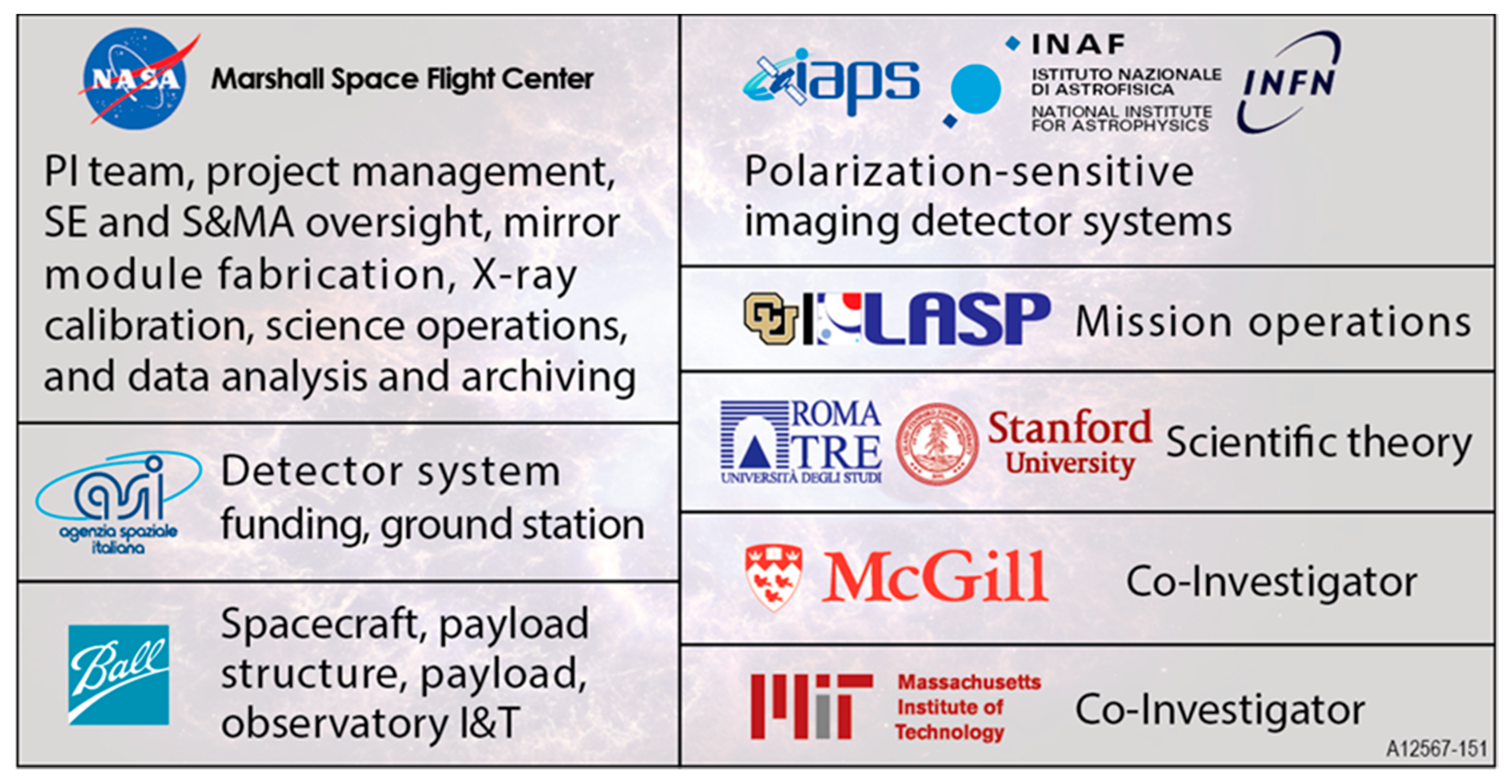
IXPE is a collaboration between NASA and ASI, the Italian Space Agency. The institutions and a brief summary of their roles is shown in Figure 10. The current list of co-investigators is given in Table 1. The list of collaborators at the time of selection is given in Table 2. The IXPE science working group, co-chaired by the project scientist, S. L. O’Dell, and Prof. G. Matt is currently establishing the procedures by which participation in IXPE will be extended beyond that listed in these tables.
The current plans for IXPE involve a Pegasus XL launch from Kwajalein Island in early 2021. IXPE will be placed into a nominal orbit of at least 540 km at 0° inclination, thus minimizing interaction with the radiation belts. The baseline mission is for two years with at least a one-year extension. ASI is providing the ground station at Malindi and IXPE will use the station at Singapore as a backup. Mission operations will be conducted by Colorado University’s Laboratory for Atmospheric and Space Physics (LASP). Science operations will take place at the Marshall Space Flight Center.
Figure 11 shows IXPE, once the boom that establishes the in-flight focal length of nominally 4-m, is deployed. Major elements of the payload and their location are identified in the figure. In what follows, we will concentrate on the optics and the polarization-sensitive detectors. The metrology camera and light emitting diodes (LEDs) are present to measure any alignment changes that might take place during launch and flight. The tip/tilt/rotate mechanism is present to readjust the alignment if necessary.
3.1. The IXPE Optics
The IXPE optics are NiCo mirror shells fabricated at MSFC using electroforming replication (see e.g., [18,19]). The design is illustrated in Figure 12. A single rigid spider is used to support 24 nested mirror shells that comprise one of three identical mirror module assemblies (MMAs). Mounting combs, as shown in the figure, provide shell attachment points. The light-weight housing is primarily for thermal control. A rear spider is also present, but is only used to limit shell vibrations during launch. The overall properties of the IXPE MMAs are summarized in Table 3.
3.2. The IXPE Detectors
A schematic of the IXPE detector is shown in Figure 13 and characteristics of each of the three detectors are given in Table 4. Figure 14 illustrates two extremely important characteristics of these detectors, namely the measurements of the modulation factor, µ, and verification of the absence of systematic effects to high precision.
3.3. The IXPE Science
IXPE opens a new window on the X-ray universe—imaging X-ray polarimetry. This provides powerful and unique capabilities as compared to all other current X-ray astronomy missions. IXPE, when compared to the polarimeters of OSO-8, will be able to reach the same sensitivity, but with an observing time that is a factor of 100 lower. Moreover, IXPE is the only observatory that can provide, simultaneously, spectral, imaging, timing, and polarization data from the sources it observes. This capability allows one to address key questions in astronomy and astrophysics and provide new scientific results and constraints for theoretical models. Amongst these questions are:
- What is the spin of an accreting stellar mass black hole?
- What are the geometry and magnetic field strength in magnetars?
- Was the black hole at the center of the Milky Way an active galactic nucleus in the recent past?
- What is the magnetic field structure in synchrotron X-ray sources?
- What are the geometries and origins of X-rays from both isolated and accreting pulsars?
For our first example of IXPE science we consider measuring black hole spin in the black hole-induced twisted space-time. The example is GRX1915+105, a micro-quasar in a binary system in an accretion-dominated state. In this case a scattering disk forms about the black hole and is fed by material from the companion star. Scattering polarizes the thermal disk emission and the twisted space-time rotates the polarization depending on the distance of the photon from the black hole. The rotation of the polarization vector is more dominant at high energies as the inner portions of the disk are hotter, producing higher energy X-rays. The impact on the polarization depends heavily on the spin of the black hole as shown in Figure 15 which shows the variation of the degree of polarization and the position angle (relative to an arbitrary zero) as a function of energy for different assumed values of the spin parameter, a. The figure also shows the results of fitting these curves assuming a 200 ksec observation with IXPE. Including priors on the disk orientation, the spin parameter can be measured to the following precision depending on the spin: a = 0.50 ± 0.04, 0.900 ± 0.008, 0.99800 ± 0.0003.
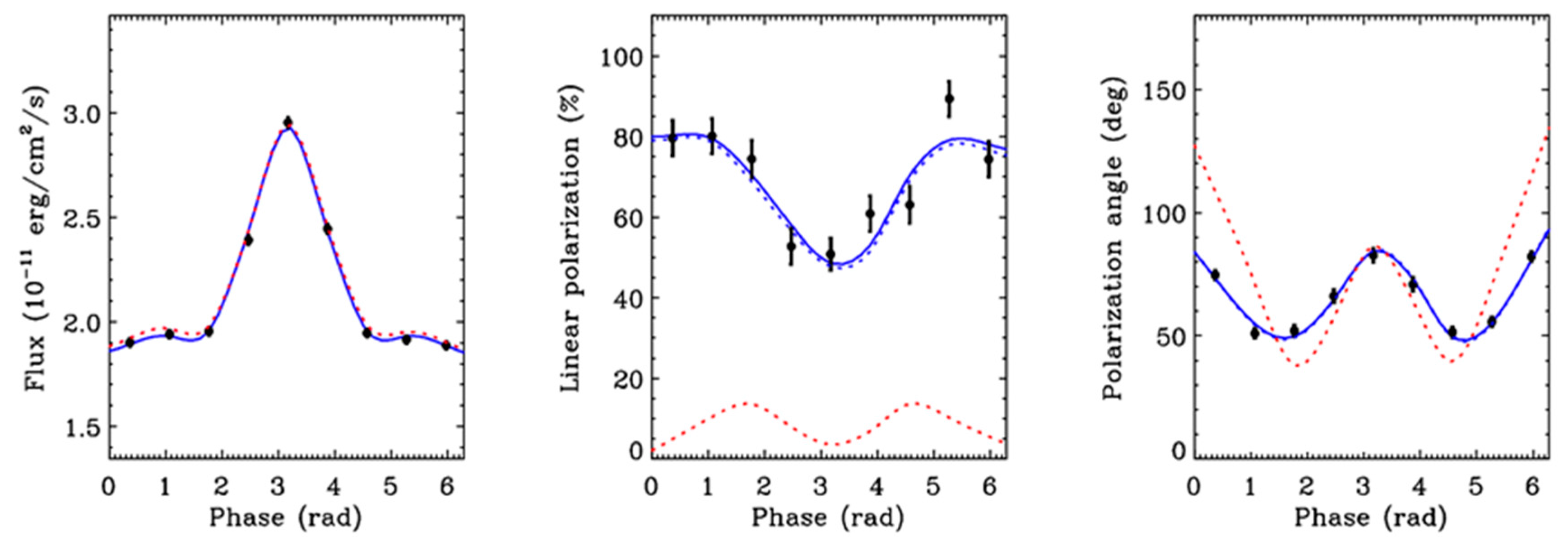
Another fascinating example of the potential of IXPE is illustrated in Figure 16 where we show the results of pulse-phase polarimetry for the 11 s pulsating magnetar 1RXS J170849.0-400910, under two conditions: (1) ignoring the effects of quantum electrodynamics (QED) in modeling the source of the pulsed emission in a super-strong magnetic field; or (2) accounting for QED. A simple light curve of intensity versus pulse phase cannot distinguish these two cases; the pulse-phase polarimetry clearly can.
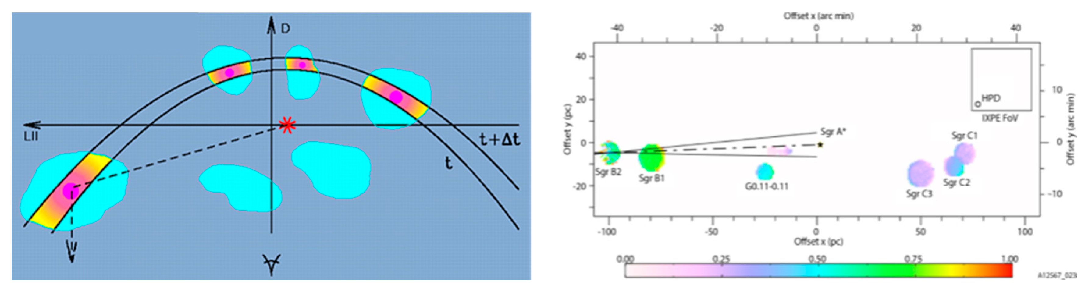
Supernova remnants and pulsar wind nebulae are obvious candidates for imaging polarimetry and many such observations will be part of the IXPE observing plan. A fascinating example of exploiting the imaging capability involves observation of the region near the fairly small (only a few million solar masses) black hole, SgR A*, at the center of our galaxy. The experiment is illustrated in Figure 17. The molecular clouds shown will reflect X-rays if emitted from SgR A*. Due to the distances involved the reflected X-rays will have been emitted by the black hole several hundred years ago. Since the scattering angle is approximately 90 degrees, the position angle of the polarized flux will point back towards SgR A* identifying it as the source of X-rays. In this case, fluxes from SgR B2 [20] would imply that SgR A* was a million times more intense just a short few hundred years ago than it is today.
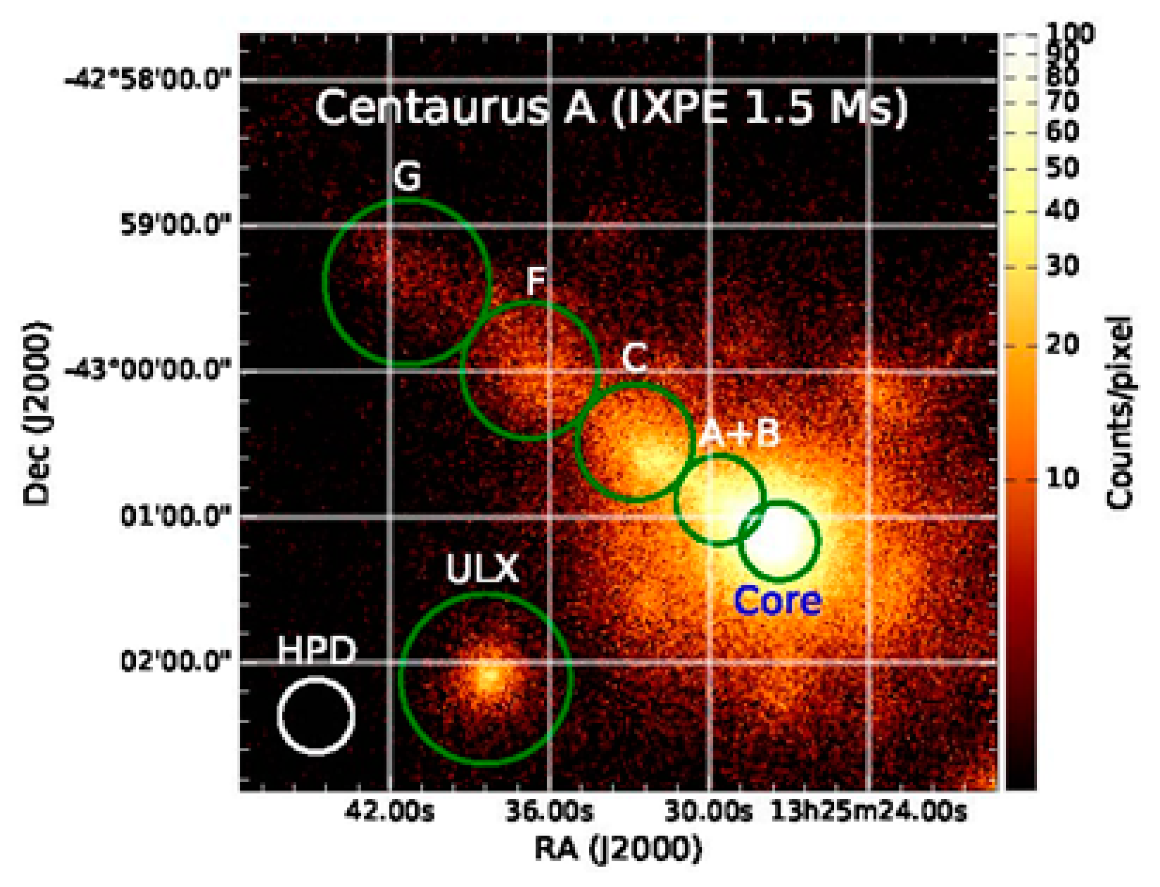
We conclude this discussion with the example of using IXPE to image and study the polarization properties of the extragalactic active galaxy, Cen A and its jet. Figure 18 illustrates a 1.5 msec observation and illustrates a number of regions which may be easily resolved. Note that the angular resolution also allows one to simultaneously study two ultra-luminous X-ray sources (one is shown) that are in the full field. Table 5 shows the minimum detectable polarization that may be achieved based on this investment of observing time. Note that the table includes the effects of dilution by unpolarized diffuse emission. This is a very important experiment for understanding the physical processes that form and maintain these X-ray-emitting jets. Radio polarization [21] implies that the field is aligned with the direction of the jet. However, different models for electron acceleration may predict different dependences in X-rays.
Conflicts of Interest
The author declares no conflict of interest.
References
- Angel, J.R.; Weisskopf, M.C. Use of Highly Reflecting Crystals for Spectroscopy and Polarimetry in X-Ray Astronomy. Astron. J. 1970, 75, 231–236. [Google Scholar] [CrossRef]
- Novick, R.; Weisskopf, M.C.; Berthelsdorf, R.; Linke, R.; Wolff, R.S. Detection of X-Ray Polarization of the Crab Nebula. Astrophys. J. 1972, 174, L1. [Google Scholar] [CrossRef]
- Weisskopf, M.C.; Cohen, G.G.; Kestenbaum, H.L.; Novick, R.; Wolff, R.S.; Landecker, P.B. The X-ray polarization experiment on the OSO-8. In Proceedings of the Symposium on X-ray Binaries, held at NASA’s Goddard Space Flight Center, Greenbelt, MD, USA, 20–22 October 1975; pp. 81–96. [Google Scholar]
- Weisskopf, M.C.; Silver, E.H.; Kestenbaum, H.L.; Long, K.S.; Novick, R. A precision measurement of the X-ray polarization of the Crab Nebula without pulsar contamination. Astrophys. J. 1978, 220, L117–L121. [Google Scholar] [CrossRef]
- Moran, P.; Shearer, A.; Mignani, R.P.; Słowikowska, A.; De Luca, A.; Gouiffès, C.; Laurent, P. Optical polarimetry of the inner Crab nebula and pulsar. Mon. Not. R. Astron. Soc. 2013, 433, 2564–2575. [Google Scholar] [CrossRef]
- Weisskopf, M.C.; Hester, J.J.; Tennant, A.F.; Elsner, R.F.; Schulz, N.S.; Marshall, H.L.; Karovska, M.; Nichols, J.S.; Swartz, D.A.; Kolodziejczak, J.J.; et al. Discovery of Spatial and Spectral Structure in the X-Ray Emission from the Crab Nebula. Astrophys. J. 2000, 536, L81–L84. [Google Scholar] [CrossRef] [PubMed]
- Weisskopf, M.C.; Kestenbaum, H.L.; Long, K.S.; Novick, R.; Silver, E.H. An upper limit to the linear X-ray polarization of Scorpius X-1. Astrophys. J. 1978, 221, L13–L16. [Google Scholar] [CrossRef]
- Silver, E.H.; Weisskopf, M.C.; Kestenbaum, H.L.; Long, K.S.; Novick, R.; Wolff, R.S. The first search for X-ray polarization in the Centaurus X-3 and Hercules X-1 pulsars. Astrophys. J. 1979, 232, 248–254. [Google Scholar] [CrossRef]
- Weisskopf, M.C.; Kestenbaum, H.L.; Long, K.S.; Novick, R.; Silver, E.H.; Wolff, R.S. Discovery of Linear X-Ray Polarization in Cygnus X-2. Bull. Am. Astron. Soc. 1976, 8, 493. [Google Scholar]
- Weisskopf, M.C.; Silver, E.H.; Kestenbaum, H.L.; Long, K.S.; Novick, R.; Wolff, R.S. Search for X-ray polarization in Cygnus X-1. Astrophys. J. 1977, 215, L65–L68. [Google Scholar] [CrossRef]
- Kaaret, P.; Novick, R.; Martin, C.; Shaw, P.; Hamilton, T.; Sunyaev, R.; Lapshov, I.; Silver, E.; Weisskopf, M.; Elsner, R. The Stellar X-ray Polarimeter—A focal plane polarimeter for the Spectrum X-Gamma mission. Opt. Eng. 1990, 29, 773–780. [Google Scholar] [CrossRef]
- Costa, E.; Piro, L.; Soffitta, P.; Massaro, E.; Matt, G.; Perola, G.C.; Giarrusso, S.; La Rosa, G.; Manzo, G.; Santangelo, A. SXRP—An X-ray polarimeter for the SPECTRUM-X-Gamma mission. Nuovo Cimento C 1992, 15, 791–799. [Google Scholar] [CrossRef]
- Elsner, R.F.; Weisskopf, M.C.; Kaaret, P.; Novick, R.; Silver, E. Off-axis effects on the performance of a scattering polarimeter at the focus of an X-ray telescope. Opt. Eng. 1990, 29, 767–772. [Google Scholar] [CrossRef]
- Austin, R.A.; Ramsey, B.D. Optical imaging chamber for X-ray astronomy. Opt. Eng. 1993, 32, 1990–1994. [Google Scholar] [CrossRef]
- Costa, E.; Soffitta, P.; Bellazzini, R.; Brez, A.; Lumb, N.; Spandre, G. An efficient photoelectric X-ray polarimeter for the study of black holes and neutron stars. Nature 2001, 411, 662–665. [Google Scholar] [CrossRef] [PubMed]
- Bellazzini, R.; Spandre, G.; Minuti, M.; Baldini, L.; Brez, A.; Cavalca, F.; Latronico, L.; Omodei, N.; Massai, M.M.; Sgro’, C.; et al. Direct reading of charge multipliers with a self-triggering CMOS analog chip with 105 k pixels at 50 μm pitch. Nucl. Instrum. Methods Phys. Res. Sect. A 2006, 566, 552–562. [Google Scholar] [CrossRef]
- Bellazzini, R.; Spandre, G.; Minuti, M.; Baldini, L.; Brez, A.; Latronico, L.; Omodei, N.; Razzano, M.; Massai, M.M.; Pesce-Rollins, M.; et al. A sealed Gas Pixel Detector for X-ray astronomy. Nucl. Instrum. Methods Phys. Res. Sect. A 2007, 579, 853–858. [Google Scholar] [CrossRef]
- Ramsey, B.D. Replicated Nickel Optics for the Hard-X-Ray Region. Exp. Astron. 2005, 20, 85–92. [Google Scholar] [CrossRef]
- O’Dell, S.L.; Atkins, C.; Broadway, D.M.; Elsner, R.F.; Gaskin, J.A.; Gubarev, M.V.; Kilaru, K.; Kolodziejczak, J.J.; Ramsey, B.D.; Roche, J.M.; et al. X-ray optics at NASA Marshall Space Flight Center. In Proceedings of the SPIE Optics + Optoelectronics, Volume 9510, EUV and X-ray Optics: Synergy between Laboratory and Space IV, Prague, Czech Republic, 15 May 2015. [Google Scholar]
- Zhang, S.; Hailey, C.J.; Mori, K.; Clavel, M.; Terrier, R.; Ponti, G.; Goldwurm, A.; Bauer, F.E.; Boggs, S.E.; Christensen, F.E.; et al. Hard X-Ray Morphological and Spectral Studies of the Galactic Center Molecular Cloud Sgr B2: Constraining Past Sgr A* Flaring Activity. Astrophys. J. 2015, 815, 132. [Google Scholar] [CrossRef]
- Goodger, J.L.; Hardcastle, M.J.; Croston, J.H.; Kraft, R.P.; Birkinshaw, M.; Evans, D.A.; Jordán, A.; Nulsen, P.E.J.; Sivakoff, G.R.; Worrall, D.M.; et al. Long-Term Monitoring of the Dynamics and Particle Acceleration of Knots in the Jet of Centaurus A. Astrophys. J. 2010, 708, 675–697. [Google Scholar] [CrossRef]
Figure 1.
(a) A single polarimeter element consisting of a block of lithium surrounded by four proportional counters; (b) schematic of the rocket payload, side view; and (c) schematic of the rocket payload, front view.
Figure 1.
(a) A single polarimeter element consisting of a block of lithium surrounded by four proportional counters; (b) schematic of the rocket payload, side view; and (c) schematic of the rocket payload, front view.

Figure 2.
Solid lines are the Thomson approximation and the dots allow for coherent and incoherent scattering angles and photoelectric absorption for the lithium blocks. (Left) Cosine of the polar scattering angle; and (right) The azimuthal scattering angle.
Figure 2.
Solid lines are the Thomson approximation and the dots allow for coherent and incoherent scattering angles and photoelectric absorption for the lithium blocks. (Left) Cosine of the polar scattering angle; and (right) The azimuthal scattering angle.

Figure 3.
Schematic of sounding rocket 17.09 which featured both lithium scattering polarimeters in the forward section of the payload and four mosaic graphite crystal Bragg polarimeters, each mounted at an average angle of 45 degrees to the incident flux and featured proportional counters as detectors. The doors opened once the payload achieved altitude.
Figure 4.
Rocket 17.09 and the science team. From left to right, Prof. Robert Novick, Director of the Columbia Astrophysics laboratory, Gabriel Epstein, graduate student for the crystal polarimeters, Prof. Martin C. Weisskopf, lead for the crystal polarimeters, Prof. Richard Wolff, lead for the lithium scattering polarimeters, and Richard Linke, graduate student for the lithium polarimeters.

Figure 5.
Photograph of the engineering model of the OSO-8 graphite crystal panel.

Figure 6.
Comparison of the position angle as measured in the optical with the OSO-8 result. The red line is the optical polarization. The black line is the OSO-8 result with errors shown in blue.
Figure 6.
Comparison of the position angle as measured in the optical with the OSO-8 result. The red line is the optical polarization. The black line is the OSO-8 result with errors shown in blue.

Figure 7.
(Left) Concept of the SXRP. Incident X-rays focused from the telescope converge onto a thin graphite crystal. Higher-energy X-rays pass through the crystal and are scattered by a block of beryllium-covered lithium. The diffracted and scattered X-rays are detected by imaging proportional counters; (right) photograph of the completed device.

Figure 8.
Schematic of the optical imaging chamber.

Figure 9.
The electron track produced by a 54 keV X-ray as imaged with the optical imaging chamber. The detector gas was a mixture of 2 atmospheres of argon (90%), methane (5%), and trimethylamine (5%). The track is about 14 mm in length. The blob at the top-right is the Auger electron cloud produced by the initial ionization.
Figure 10.
Major institutions involved in IXPE. Abbreviations: PI = principal investigator, SE = systems engineering, S&MA = safety and mission assurance, I&T = integration and test.
Figure 10.
Major institutions involved in IXPE. Abbreviations: PI = principal investigator, SE = systems engineering, S&MA = safety and mission assurance, I&T = integration and test.

Figure 11.
Schematic rendering of IXPE deployed with the major elements identified.

Figure 12.
Schematic of a single IXPE mirror module assembly (MMA). (a) Entire MMA; (b) close-up of the front spider; and (c) close-up of an alignment comb.
Figure 12.
Schematic of a single IXPE mirror module assembly (MMA). (a) Entire MMA; (b) close-up of the front spider; and (c) close-up of an alignment comb.
Figure 13.
Schematic of the IXPE detector. Abbreviations: GEM = gas electron multiplier; ADC = analog to digital convertor; DME = dimethyl ether.
Figure 13.
Schematic of the IXPE detector. Abbreviations: GEM = gas electron multiplier; ADC = analog to digital convertor; DME = dimethyl ether.
Figure 14.
(Left) The modulation factor, µ, as a function of energy. The solid line is based on Monte-Carlo simulations. The colored symbols are based on measurements at different times. The dotted lines are simple linear connections; (upper right) Measurements of a 99%-polarized source at 3.7 keV; (lower right) Measurements of an unpolarized source at 5.9 keV.
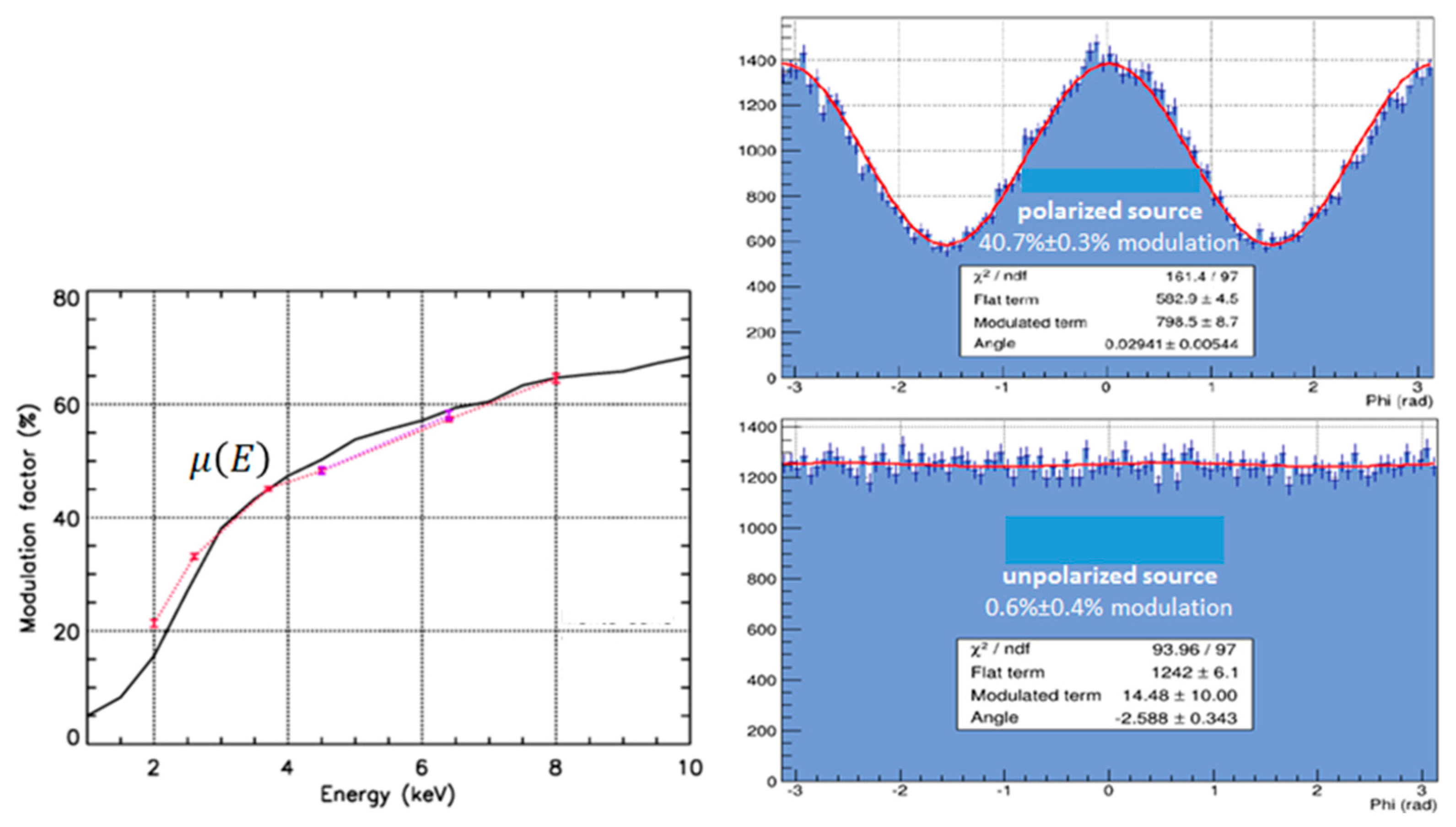
Figure 15.
(Left) Linear polarization versus energy for various black hole spin parameters; (right) Position angle with respect to an arbitrary reference. Dotted lines are based on model calculations. Solid lines are fits to the data based on a 200 ksec IXPE observation.
Figure 15.
(Left) Linear polarization versus energy for various black hole spin parameters; (right) Position angle with respect to an arbitrary reference. Dotted lines are based on model calculations. Solid lines are fits to the data based on a 200 ksec IXPE observation.
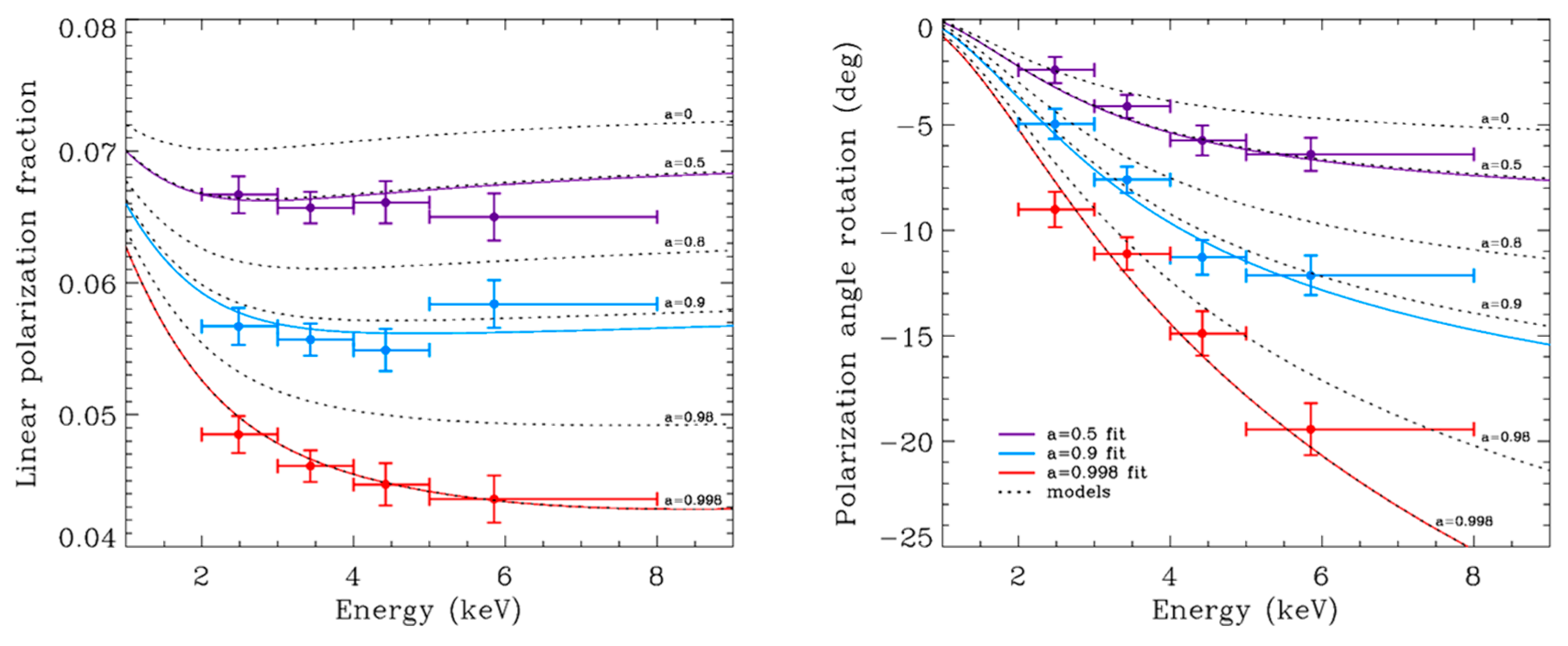
Figure 16.
Left to right: flux, degree of polarization, and position angle, all versus the pulse phase for 1RXS J170849.0-400910. Blue and red curves represent QED accounted for and not accounted for, respectively. Data points and errors are for a 250-ksec observation.
Figure 16.
Left to right: flux, degree of polarization, and position angle, all versus the pulse phase for 1RXS J170849.0-400910. Blue and red curves represent QED accounted for and not accounted for, respectively. Data points and errors are for a 250-ksec observation.

Figure 17.
(Left) Looking down on the galactic center. The red asterisk is Sagittarius A* and the blue object to the left is a representation of the molecular cloud SgR B2. X-rays emitted by SgR A* may be scattered to IXPE by SgR B2; (right) View of the galactic center from IXPE. The square in the top right of the figure represents the size of the IXPE field of view and the HPD is the half-power-diameter showing that SgR B2 is clearly resolved. The dashed line pointing back to SgR A* represents the position angle of the scattered X-rays and the solid lines represent the measured uncertainty.

Figure 18.
IXPE image of Cen A. The half-power diameter (HPD) is the small circle on the left. An ultra-luminous source of X-rays (ULX) is identified together with the core of Cen A and a number knots. The minimum detectable polarizations based on a 1.5 msec IXPE observation are given in Table 5.
Figure 18.
IXPE image of Cen A. The half-power diameter (HPD) is the small circle on the left. An ultra-luminous source of X-rays (ULX) is identified together with the core of Cen A and a number knots. The minimum detectable polarizations based on a 1.5 msec IXPE observation are given in Table 5.


Table 1.
IXPE co-Investigators and roles.
| L. Baldini | Co-I and PI for INFN/Pisa |
| R. Bellazzini | Senior Co-I |
| E. Costa | Senior Co-I |
| R. Elsner | Co-I |
| V. Kaspi | Co-I and co-chair of the SWG |
| J. Kolodziejczak | Co-I |
| L. Latronico | Co-I and PI for INFN/Pisa |
| H. Marshall | Co-I |
| G. Matt | Co-I and extragalactic theory lead |
| F. Mulieri | Co-I |
| S.L. O’Dell | Co-I and Project scientist |
| B.D. Ramsey | Deputy PI |
| R.W. Romani | Co-I and galactic theory lead |
| P. Soffitta | Co-I and Italian PI |
| A.Tennant | Co-I |
Table 2.
IXPE collaborators.
| W. Baumgartner | L. Pacciani |
| A. Brez | G. Pavlov |
| N. Bucciantini | M. Pesce-Rollins |
| E. Churazov | P.-O. Petrucci |
| S. Citrano | M. Pinchera |
| E. Del Monter | J. Poutanen |
| N. Di Lalla | M. Razzano |
| I. Donnarumma | A. Rubini |
| M. Dovčiak | M. Salvati |
| Y. Evangelista | C. Sgrò |
| S. Fabiani | F. Spada |
| R. Goosmann | G. Spandre |
| S. Gunji | L. Stella |
| V. Karas | R. Sunyaev |
| M. Kuss | R. Taverna |
| A. Manfreda | R. Turolla |
| F. Marin | K. Wu |
| M. Minuti | S. Zane |
| N. Omodei | D. Zanetti |
Table 3.
MMA properties.
| Parameter | Value |
|---|---|
| Number of mirror modules | 3 |
| Number of shells per mirror module | 24 |
| Focal length | 4001 mm |
| Total shell length | 600 mm |
| Range of shell diameters | 162–272 mm |
| Range of shell thicknesses | 0.18–0.25 mm |
| Shell material | Electroformed nickel–cobalt alloy |
| Effective area per mirror module with thermal shields | 209 cm2 (@ 2.3 keV); >230 cm2 (3–6 keV) |
| Angular resolution (HPD) | ≤25 arcsec |
| Field of view (detector limited) | 12.9 arcmin square |
Table 4.
Detector parameters.
| Parameter | Value |
|---|---|
| Sensitive area | 15 mm × 15 mm |
| Fill gas and composition | He/DME (20/80) @ 1 atm |
| Detector window | 50-µm thick beryllium |
| Absorption and drift region depth | 10 mm |
| GEM (gas electron multiplier) | copper-plated 50-µm liquid-crystal polymer |
| GEM hole pitch | 50 µm triangular lattice |
| Number ASIC readout pixels | 300 × 352 |
| ASIC pixelated anode | Hexagonal @ 50-µm pitch |
| Spatial resolution (FWHM) | ≤123 µm (6.4 arcsec) @ 2 keV |
| Energy resolution (FWHM) | 0.54 keV @ 2 keV (∝ √E) |
Table 5.
MDP for different regions of Cen A for 1.5 msec.
| Region | MDP99 |
|---|---|
| Core | <7.0% |
| Jet | 10.9% |
| Knot A + B | 17.6% |
| Knot C | 16.5% |
| Knot F | 23.5% |
| Knot G | 30.9% |
| ULX | 14.8% |
© 2018 by the author. Licensee MDPI, Basel, Switzerland. This article is an open access article distributed under the terms and conditions of the Creative Commons Attribution (CC BY) license (http://creativecommons.org/licenses/by/4.0/).
Share and Cite
MDPI and ACS Style
Weisskopf, M.C. An Overview of X-Ray Polarimetry of Astronomical Sources. Galaxies 2018, 6, 33. https://doi.org/10.3390/galaxies6010033
AMA Style
Weisskopf MC. An Overview of X-Ray Polarimetry of Astronomical Sources. Galaxies. 2018; 6(1):33. https://doi.org/10.3390/galaxies6010033
Chicago/Turabian StyleWeisskopf, Martin C. 2018. "An Overview of X-Ray Polarimetry of Astronomical Sources" Galaxies 6, no. 1: 33. https://doi.org/10.3390/galaxies6010033
Note that from the first issue of 2016, this journal uses article numbers instead of page numbers. See further details here.