The Variable Rotation Measure Distribution in 3C 273 on Parsec Scales

Physics Department, Brandeis University, Waltham, MA 02453, USA
Galaxies 2018, 6(1), 5; https://doi.org/10.3390/galaxies6010005
Submission received: 15 September 2017
/
Revised: 17 December 2017
/
Accepted: 18 December 2017
/
Published: 5 January 2018
(This article belongs to the Special Issue Polarised Emission from Astrophysical Jets)
Abstract
:We briefly review how opacity affects the observed polarization in synchrotron emitting jets. We show some new multi-frequency observations of 3C 273 made with the VLBA in 1999–2000, which add significantly to the available rotation measure (RM) observations of this source. Our findings can be summarized as follows: (1) The transverse gradient in RM is amply confirmed. This implies a toroidal component to the magnetic field, which in turn requires a current of 1017–1018 A flowing down the jet. (2) The net magnetic field in the jet is longitudinal; however, whether or not the longitudinal component is vector-ordered is an open question. (3) The RM distribution is variable on timescales of months to years. We attribute this to the motion of superluminal components behind a turbulent Faraday screen that surrounds the jet. (4) Finally, we suggest that Faraday rotation measurements at higher resolution and higher frequencies, with the Event Horizon Telescope, may enable useful constraints to be placed on the accretion rate onto the central black hole.
1. The Effect of Opacity on Polarization
It is well known that the fractional linear polarization, m, of optically thin synchrotron radiation in a uniform magnetic field is given by m = (p + 1)/(p + 7/3) (e.g., [1]), where p is the slope of the power law electron energy distribution, and is related to the spectral index, α, (defined as ) by p = 2α + 1. For typical values of p between 2 and 3, the value of m is between 69% and 75%. Fractional polarizations this high are rarely seen, and this is usually attributed to a partially disordered magnetic field.
The effect of opacity on polarization is not as widely known as it should be, so it is useful to review it briefly here. Let us assume that our coordinate system is oriented such that the polarization is completely represented by Stokes Q (and U = 0). As the optical depth increases, Q steadily decreases, eventually passing through zero and becoming negative. This corresponds to a change of 90° in the EVPA, and at large enough optical depth, the fractional polarization becomes m = 3/(6p + 13). This is only 10–12% in a uniform field and is even less in a partially disordered field.
An important question is at what optical depth does the EVPA flip by 90°? It is not, as is sometimes assumed, at τ = 1. The critical optical depth is in fact between 6 and 7, depending weakly on the spectral index (see Figure 1a). This and the two following plots are calculated from expressions in Chapter 3 of [1]. Figure 1a uses Equation (3.79) in [1], after correcting an obvious typesetting error. At the critical optical depth plotted in Figure 1a, the fractional polarization is zero; it rises to its asymptotic value (10–12%) and the 90° EVPA flip becomes visible only at significantly larger optical depths. At such high opacity, the total intensity is greatly depressed and therefore so is the polarized intensity. Because the edges of a jet or other compact component are always optically thin (because of the short path length), it is unclear if optically thick polarization has ever actually been observed in real radio sources.
Note also that the 90° flip in EVPA only occurs in Faraday-thin sources. If a source is Faraday-thick, then the EVPA changes by only 45°, whether it is optically thick or thin. (For the connection between Faraday depth and rotation measure, see Equations (1) and (2) in [2].) The dependence of EVPA on both Faraday depth and optical depth is shown in Figure 1b for a cylindrical geometry. Since the vertical axis in Figure 1b could equally well be labeled as λ2, this demonstrates that it is not meaningful to calculate a rotation measure if a source is Faraday-thick. Some of these results have been presented [2,3], but both papers only considered optically thin sources.
It is obvious that the peak in the I map and the peak in the P map are at significantly different core distances. This difference is a measure of the gradient in optical depth along the jet and is very similar to what is measured by the core-shift technique [6,7], which measures the position of the peak in total intensity as a function of frequency. It can also be seen in Figure 2 that only a tiny region close to the apex of the jet exhibits full optically thick polarization with a 90° change in EVPA. This region makes a negligible contribution to the measured core polarization, especially if the core polarization is measured at the total intensity peak.
2. New VLBA Images of 3C 273, and the Variable Transverse Gradients of Rotation Measure
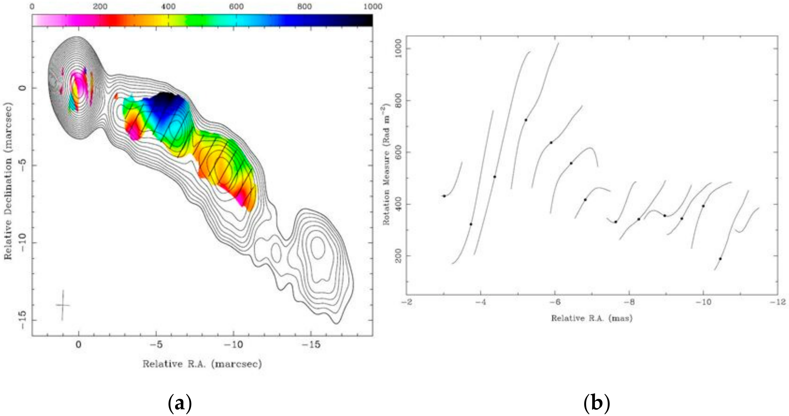
The first observation of a transverse gradient of rotation measure in the pc-scale jet of 3C 273 was by [8]. It has since been confirmed by [9,10,11,12]. It has also been seen in a number of other sources (e.g., [13] and references therein). To the body of observations of 3C 273, we add those by Chen [14]. Chen observed 3C 273 with the VLBA at 4 epochs between 1999.26 and 2000.04, at 8, 15, 22, and 43 GHz. Full results will be reported elsewhere, but in Figure 3 and Figure 4, we show transverse gradients in rotation measure and in fractional polarization taken from multiple cuts of the stacked images.
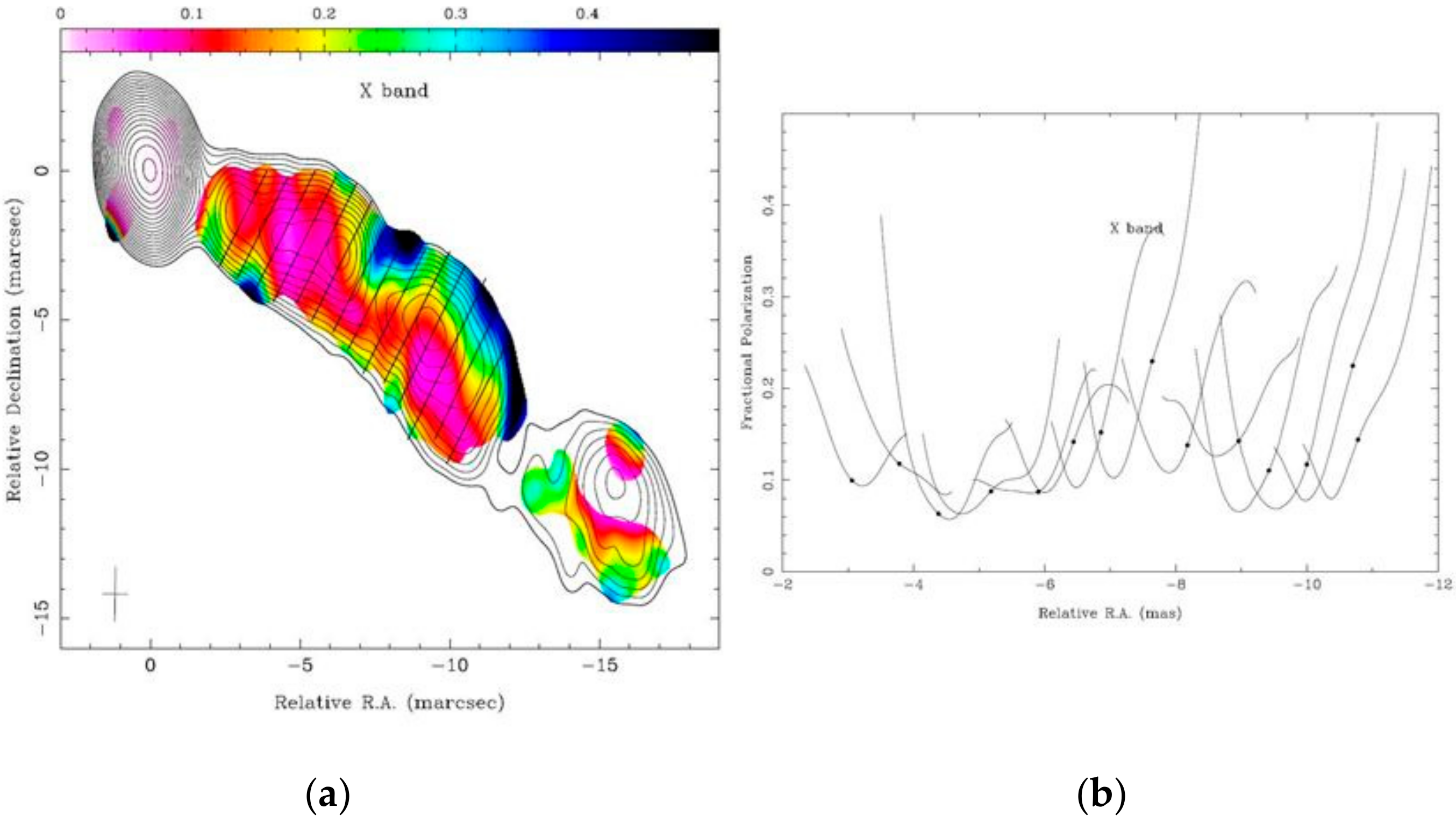
In Figure 4, we show the distribution of fractional polarization, together with 14 transverse cuts in fractional polarization. The minimum in fractional polarization near the center of the jet is also a persistent feature, best seen in the movie sequence of images on the MOJAVE website [15], and was first remarked on by [10]. It is not a Faraday effect, but a simple consequence of the magnetic field geometry, where the toroidal and longitudinal field components give comparable but orthogonal polarizations.
The rotation measure corrected zero wavelength EVPA distribution is not shown here, but can be found in [8,10,16]. Results show that the net magnetic field direction is persistently and predominantly aligned with the jet.
We have compiled all the milliarcsecond-scale RM gradient observations in the literature, including those from Chen’s thesis. These are shown in Table 1. In Column 4, the “Ridge RM” is measured at the peak in the total intensity distribution.
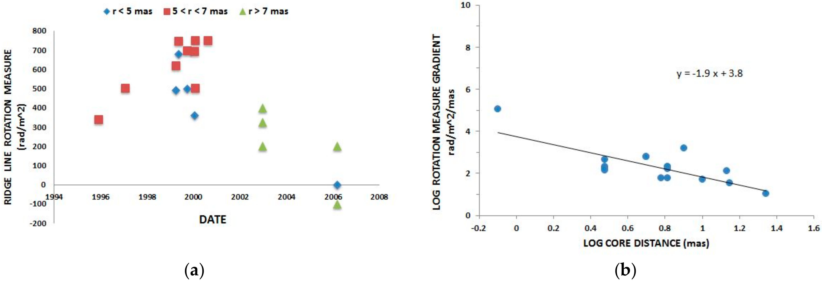
The observations listed in Table 1 form a very under-sampled data set, where the ridge RM and the RM gradient both vary with epoch and with core distance. In Figure 5, we take a first look at two of the more obvious trends.
We can see from Figure 5a that the RM in the center of the jet is variable over a range of different timescales. The general increase in RM between 1996 and 2000, followed by a decline over the next six years show variability on a timescale of years. The cluster of points around 2000—many of them new data points from [14]—show variability on the timescale of months. (Note that the large vertical scatter represents real month-to-month variability rather than measurement errors. The measurements are made on the ridge line of the jet, where the total intensity is at a maximum, and all of them have good signal-to-noise ratios.).
The RM variability cannot be attributed to the motion of emission line clouds across the line of sight, because they move too slowly [18]. However, the superluminal components in the jet certainly do move fast enough. We suggest, as have many others, that most of the Faraday screen is close to the jet, either as a sheath of plasma surrounding the jet or as a turbulent boundary layer where the jet interacts with the ambient medium. The superluminal components then act as moving probes of the Faraday screen. Their locations are accurately tracked by the MOJAVE program [19], and see [20], so it may be possible, given sufficient observations, to map the screen itself or at least to determine its statistical properties. In this picture, the range of time scales for RM variability correspond to a range of physical scale sizes for the fluctuations in the Faraday screen. However, if the screen itself is time-variable, then elucidating its structure will be very difficult.
In Figure 5b, we look at how the RM gradient depends on core distance. Clearly the gradient increases as the core distance decreases, but this conclusion depends strongly on the end data points. The rightmost data point is from [9]. The leftmost data point is from [11], based on simultaneous observations at 7 mm and 3.5 mm wavelengths. Important support for very high RMs close to the core is given by the authors of [21], who observed 3C 273 with ALMA at a wavelength of 1 mm and measured an RM of 3.8 × 10⁵ rad/m2. (They could not, of course, resolve the jet with ALMA, so this value corresponds most closely to the ridge RMs in Column 4 of Table 1.)
3. The Current in the Jet
The usual interpretation of the transverse RM gradient is that it implies a toroidal component to the magnetic field (e.g., [8]). Whether or not the net field is helical depends on whether or not the longitudinal component of the field is vector-ordered (see below). By Ampère’s law, a toroidal magnetic field requires that a current flows down the jet. If the total jet current is Ijet, then the field at the surface of a jet of radius R is B(R) = μ0 Ijet/2πR, where μ0 is the permeability of free space. Outside the jet, the magnetic field is B(r) = B(R)·R/r, where r is the radial coordinate. Inside the jet, if the current density is uniform, the current generates a toroidal component equal to B(R)·r/R. The current therefore generates both part of the field (in conjunction with the longitudinal component) that gives rise to synchrotron radiation from the jet and the magnetic field in the plasma surrounding the jet that gives rise to the RM gradient.
Jet currents are an inevitable consequence of toroidal magnetic fields. Inserting typical values for the magnetic field (see Column 6 of Table 1 in [22], where the magnetic field at a distance of 1 pc from the black hole is typically in the 0.2–1.5 G range) and the jet opening angle from [7], we expect currents in the 1017–1018 A range. There is now evidence that these currents propagate to kpc scales, perhaps even to the hotspots [23,24,25]. According to [24], the conventional current tends to flow inward on pc scales and outward on kpc scales. They identify these with the jet current and with the return current, respectively (see their Figure 1). It is interesting that, on pc scales, 3C 273 may be an exception to this rule.
4. The Structure of the Magnetic Field in the Jet
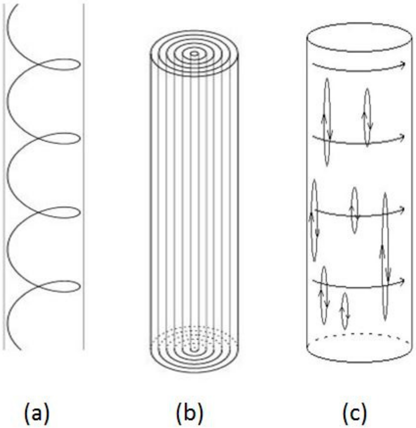
Any model for the structure of the magnetic field in 3C 273 must reproduce at least three observational features. These are (1) the transverse gradient in rotation measure, (2) the net longitudinal field, and (3) the minimum in fractional polarization in the center of the jet. The RM gradient implies a toroidal component to the magnetic field. This is frequently called a helical field, but it is only so if the longitudinal component is vector-ordered. A helical field can reproduce (2) if the pitch angle is small enough (<45°). This is certainly possible, but there are two difficulties. The first is that a helix exhibits side–side asymmetry unless viewed from 90° in the jet frame (see Figure 6a). It is not unreasonable that the viewing angle is near 90° since this is the angle that maximizes superluminal motion for a given jet velocity, but it is not reasonable to expect it to be 90° in general. In fact, 3C 273 does exhibit some side–side asymmetry—the north side of the jet is more strongly polarized than the south side—but that may also be affected by the jet curvature. This was discussed in [15], where it was pointed out that the asymmetries in polarization, total intensity, and spectral index were consistent with the expectations of the helical magnetic field model discussed in [26]. The second, perhaps more important, difficulty for a helical field is that, as the jet expands, the pitch angle must increase due to conservation of magnetic flux, and so the apparent magnetic field may start off longitudinal and then become transverse farther downstream. The corresponding fractional polarization will steadily decrease down the jet, pass through zero when the pitch angle is 45°, and then increase again. I have not found any examples of such behavior in the MOJAVE sample.
The longitudinal component does not have to be vector-ordered. Two examples of net longitudinal fields that are not vector-ordered are (1) compressed tangled fields (often called Laing sheets) wrapped around the axis of the jet (see Figure 6b) and (2) tangled magnetic fields stretched along the jet axis by transverse velocity shear (see Figure 6c). The latter can be compared to a Laing sheet [27] where a tangled field is stretched rather than compressed. Neither of these suffer from the problems outlined above for a helical field. They also straightforwardly produce a minimum in fractional polarization in the center of the jet (though a helical field can do so too).
5. How the Faraday Screen Changes with Distance from the Core
According to Figure 5b, the RM transverse gradient varies roughly with (core distance)−1.9, though the scatter in Figure 5b is such that this value is not well determined. The leftmost point in Figure 5b suggests that closer to the core, the slope may well be steeper. That the RM gradient (and the ridge line RM) decrease with increasing core distance is not unexpected, but modeling them is not necessarily straightforward. Even if the magnetic field outside the jet is considered known (see Section 3), we do not know the distribution of the ionized gas. A sheath or turbulent boundary layer surrounding the jet is possible, as are an inward accretion flow or an outward flowing wind. We also do not know the velocity field of the plasma. This is relevant because the usual formula for Faraday rotation applies in the remaining frame of the plasma.
Conflicts of Interest
The authors declare no conflict of interest.
References
- Pacholczyk, A.G. Radio Astrophysics; W. H. Freeman: San Francisco, CA, USA, 1970; pp. 99–107. [Google Scholar]
- Burn, B.J. On the depolarization of discrete radio sources by Faraday dispersion. Mon. Not. R. Astron. Soc. 1966, 133, 67–83. [Google Scholar] [CrossRef]
- Cioffi, D.F.; Jones, T.W. Internal Faraday rotation effects in transparent synchrotron sources. Astron. J. 1980, 85, 368–375. [Google Scholar] [CrossRef]
- Cobb, W.K. Theoretical Studies of the Polarization and Variability of Inhomogeneous Relativistic Jets. Ph.D. Thesis, Brandeis University, Waltham, MA, USA, 1993. [Google Scholar]
- Blandford, R.D.; Königl, A. Relativistic jets as compact radio sources. Astrophys. J. 1979, 232, 34–48. [Google Scholar] [CrossRef]
- Lobanov, A.P. Ultracompact jets in active galactic nuclei. Astron. Astrophys. 1998, 330, 79–89. [Google Scholar]
- Pushkarev, A.B.; Hovatta, T.; Kovalev, Y.Y.; Lister, M.L.; Lobanov, A.P.; Savolainen, T.; Zensus, J.A. MOJAVE: Monitoring of Jets in Active galactic nuclei with VLBA Experiments. IX. Nuclear opacity. Astron. Astrophys. 2012, 545, 113–128. [Google Scholar] [CrossRef]
- Asada, K.; Inoue, M.; Uchida, Y.; Kameno, S.; Fujisawa, K.; Iguchi, S.; Mutoh, M. A Helical Magnetic Field in the Jet of 3C 273. Pub. Astron. Soc. Jpn. 2002, 54, L39–L43. [Google Scholar] [CrossRef]
- Asada, K.; Inoue, M. A follow-up RM observation for helical magnetic field in 3C273. In Proceedings of the 7th Symposium of the European VLBI Network on New Developments in VLBI Science and Technology, Toledo, Spain, 12–15 October 2004; Bachiller, R., Colomer, F., Desmurs, J.F., de Vicente, P., Eds.; Observatorio Astronomico Nacional of Spain: Madrid, Spain, 2004; pp. 65–68. [Google Scholar]
- Zavala, R.T.; Taylor, G.B. Faraday Rotation Measure Gradients from a Helical Magnetic Field in 3C 273. Astrophys. J. 2005, 626, L73–L76. [Google Scholar] [CrossRef]
- Attridge, J.M.; Wardle, J.F.C.; Homan, D.C. Concurrent 43 and 86 GHz Very Long Baseline Polarimetry of 3C 273. Astrophys. J. 2005, 633, L85–L88. [Google Scholar] [CrossRef]
- Hovatta, T.; Lister, M.L.; Aller, M.F.; Aller, H.D.; Homan, D.C.; Kovalev, Y.Y.; Pushkarev, A.B.; Savolainen, T. Faraday rotation in the MOJAVE blazars: 3C 273 a case study. J. Phys. Conf. Ser. 2012, 355, 2008–2013. [Google Scholar] [CrossRef]
- Gabuzda, D.C.; Roche, N.; Kirwan, A.; Knuettel, S.; Nagle, M.; Houston, C. Parsec scale Faraday-rotation structure across the jets of nine active galactic nuclei. Mon. Not. R. Astron. Soc. 2017, 472, 1792–1801. [Google Scholar] [CrossRef]
- Chen, T. VLBI and VSOP Study of Two Quasar Jets. Ph.D. Thesis, Brandeis University, Waltham, MA, USA, 2005. [Google Scholar]
- The Mojave Program. Available online: http://www.physics.purdue.edu/astro/MOJAVE/sourcepages/1226+023.shtml (accessed on 3 January 2018).
- Hovatta, T.; Lister, M.L.; Aller, M.F.; Aller, H.D.; Homan, D.C.; Kovalev, Y.Y.; Pushkarev, A.B.; Savolainen, T. MOJAVE: Monitoring of Jets in Active Galactic Nuclei with VLBA Experiments. VIII. Faraday Rotation in Parsec-scale AGN Jets. Astron. J. 2012, 144, 105–139. [Google Scholar] [CrossRef]
- Zavala, R.T.; Taylor, G.B. Time-Variable Faraday Rotation Measures of 3C 273 and 3C 279. Astrophys. J. 2001, 550, L147–L150. [Google Scholar] [CrossRef]
- Asada, K.; Inoue, M.; Kameno, S.; Nagai, H. Time Variation of the Rotation Measure Gradient in the 3C 273 Jet. Astrophys. J. 2008, 675, 79–82. [Google Scholar] [CrossRef]
- Romero, G.E.; Boettcher, M.; Markoff, S.; Tavecchio, F. MOJAVE. X. Parsec-scale Jet Orientation Variations and Superluminal Motion in Active Galactic Nuclei. Astron. J. 2013, 146, 120–142. [Google Scholar] [CrossRef]
- The Mojave Program Available online:. Available online: http://www.physics.purdue.edu/astro/MOJAVE/animated/1226+023.i.mpg (accessed on 3 January 2018).
- Hovatta, T.; O’Sullivan, S.; Marti-Vidal, I.; Savolainen, T.; Tchekhovskoy, A. Astron. Astrophys. 2018. submitted.
- Zamaninasab, M.; Clausen-Brown, E.; Savolainen, T.; Tchekhovskoy, A. Dynamically important magnetic fields near accreting supermassive black holes. Nature 2014, 510, 126–128. [Google Scholar] [CrossRef] [PubMed]
- Kronberg, P.P.; Lovelace, R.V.; Lapenta, G.; Colgate, S.A. Measurement of the Electric Current in a kpc-scale Jet. Astrophys. J. 2011, 741, L15–L18. [Google Scholar] [CrossRef]
- Christodoulou, D.M.; Gabuzda, D.C.; Knuettel, S.; Contopoulos, I.; Kazanas, D.; Coughlan, C.P. Dominance of outflowing electric currents on decaparsec to kiloparsec scales in extragalactic jets. Astron. Astrophys. 2016, 591, A61–A71. [Google Scholar] [CrossRef]
- Contopoulos, I. Electric currents along astrophysical jets. Galaxies 2017, 5, 71. [Google Scholar] [CrossRef]
- Clausen-Brown, E.; Lyutikov, M.; Kharb, P. Signatures of large-scale magnetic fields in active galactic nuclei jets: Transverse asymmetries. Mon. Not. R. Astron. Soc. 2011, 415, 2081–2092. [Google Scholar] [CrossRef]
- Laing, R.A.; Canvin, J.R.; Bridle, A.H. Magnetic fields in jets: Ordered or disordered? Astron. Nachr. 2006, 327, 523–526. [Google Scholar] [CrossRef]
- Mizrahi, J. A Model for the Magnetic Field in the Jet of the Quasar 3C273. Bachelor’s Thesis, Brandeis University, Waltham, MA, USA, Unpublished work. 2007. [Google Scholar]
- Marrone, D.P.; Moran, J.M.; Zhao, J.H.; Rao, R. An Unambiguous Detection of Faraday Rotation in Sagittarius A. Astrophys. J. 2007, 654, L57–L60. [Google Scholar] [CrossRef]
- Fish, V.; Akiyama, K.; Bouman, K.L.; Chael, A.A.; Johnson, M.D.; Doeleman, S.S.; Blackburn, L.; Wardle, J.F.; Freeman, W.T. Event Horizon Telescope Collaboration. Observing—And Imaging—Active Galactic Nuclei with the Event Horizon Telescope. Galaxies 2016, 4, 54. [Google Scholar] [CrossRef]
Figure 1.
(a) The critical optical depth, τ, at which the EVPA changes by 90° as a function of electron energy spectral index, p. (b) The fractional polarization (contours) and EVPA (constant length tick marks) as a function of optical depth, τ, and Faraday depth, τF, integrated over a cylinder, for p = 2.5. The lower left portion of this diagram represents optically thin, Faraday-thin emission. The lower right portion shows Faraday-thin, optically thick emission. The 90° change in the EVPA is only plainly visible for optical depths >10. Note that, in the top portion of the diagram, increasing Faraday depth limits the EVPA rotation to 45°. Figure 1a,b are copied from [4].

Figure 2.
Contours of total intensity (left) and polarized intensity (right) for a resolved Blandford–Königl jet with a toroidal magnetic field. The cross marks the position of unit optical depth. The polarization tick marks are EVPAs. Figure 2 is also copied from [4].
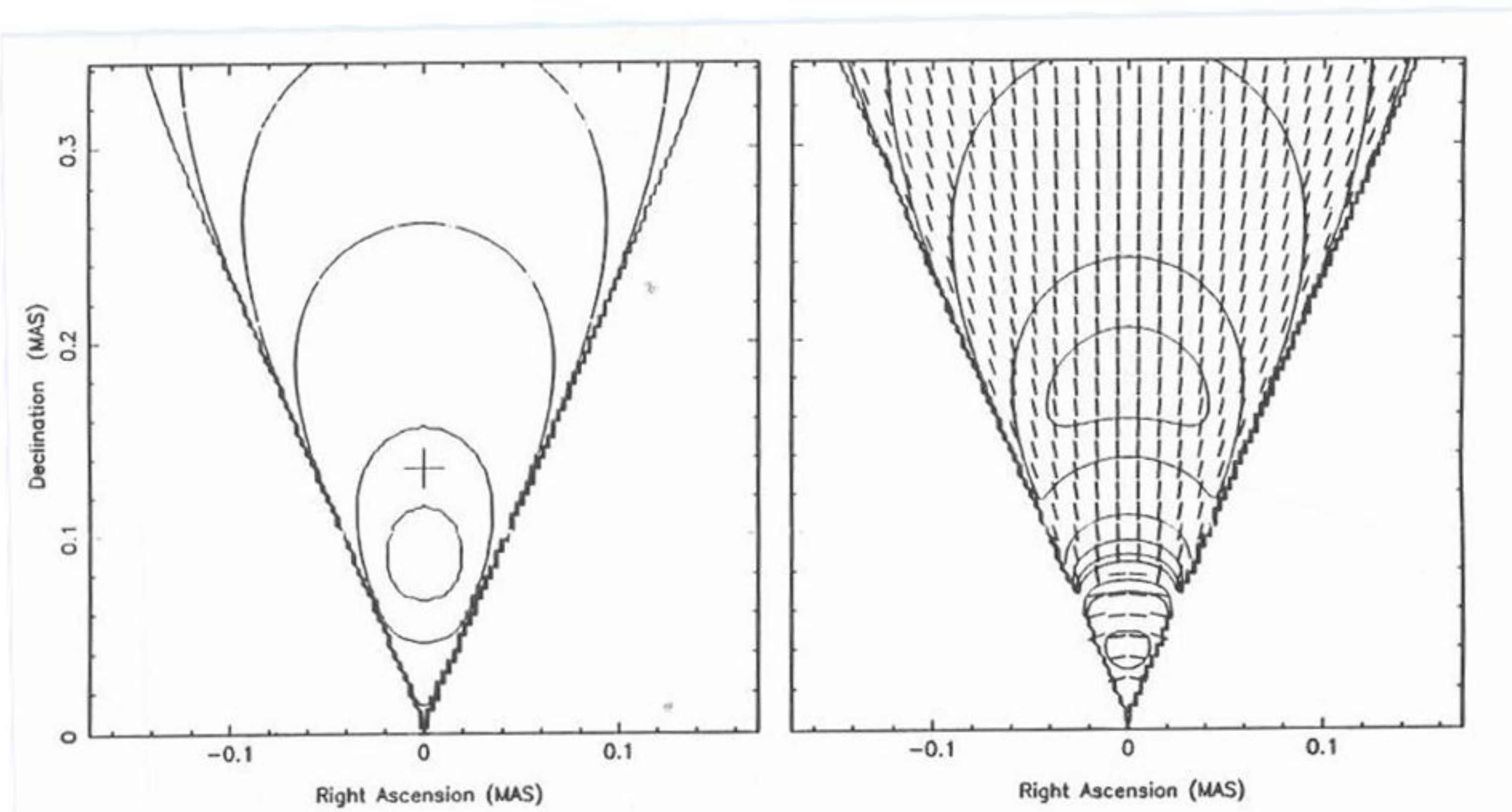
Figure 3.
(a) Rotation measure distribution from the stacked images at 4 frequencies, superposed on the 8 GHz total intensity image. (b) Fourteen transverse cuts in rotation measure. It is clear that the transverse gradient in rotation measure can be seen down the length of the jet. The dots indicate the peaks in total intensity for each cut. These correspond to the ridge line RMs in Table 1.

Figure 4.
(a) Fractional polarization of the stacked images at 8 GHz. (b) Fourteen transverse cuts in fractional polarization. Note that the minimum in fractional polarization (red) is consistently near the center of the jet.
Figure 4.
(a) Fractional polarization of the stacked images at 8 GHz. (b) Fourteen transverse cuts in fractional polarization. Note that the minimum in fractional polarization (red) is consistently near the center of the jet.

Figure 5.
(a) Ridge line rotation measures as a function of observing epoch. Because the RM also varies with core-distance, we have split the measurements into three ranges of core-distance, as given in the legend. (b) The dependence of the transverse RM gradient on projected distance from the core measured in milliarcseconds. The regression line has a formal slope of −1.9, but with a large and uncertain error because the scatter about that line is largely due to variability.

Figure 6.
Three possible magnetic field configurations discussed in the text. (a) a vector-ordered helix. The side to side asymmetry is obvious if the jet is not viewed from a direction perpendicular to its axis; (b) two-dimensional field sheets wrapped around the jet axis; (c) a toroidal field plus longitudinal loops. Both configurations (b,c) reproduce the observed polarization properties of jets, while avoiding some of the problems associated with completely vector-ordered fields (see text). Figure 6a,b are taken from [27]. Figure 6c is taken from [28].


Table 1.
Compilation of RM observations of 3C 273 at milliarcsecond resolution.
| Date | Frequency GHz | Core Distance 1 Mas | Ridge RM Rad/m2 | RM Gradient Rad/m2/Mas | Reference |
|---|---|---|---|---|---|
| 1995.92 | 4.7–8.6 | 6 | 340 | 60 | [8] |
| 1997.07 | 8.1–43.2 | 5 | 500 | [17] | |
| 1999.26 | 8.1–22.2 | 3 | 489 | 185 | [14] |
| 1999.26 | 8.1–22.2 | 6.5 | 619 | 61 | [14] |
| 1999.37 | 8.1–22.2 | 3 | 679 | 207 | [14] |
| 1999.37 | 8.1–22.2 | 6.5 | 746 | 160 | [14] |
| 1999.74 | 8.1–22.2 | 3 | 497 | 170 | [14] |
| 1997.74 | 8.1–22.2 | 6.5 | 695 | 211 | [14] |
| 2000.04 | 8.1–22.2 | 3 | 358 | 137 | [14] |
| 2000.04 | 8.1–22.2 | 6.5 | 393 | 213 | [14] |
| 2000.07 | 12.1–22.2 | 5 | 750 | 600 | [10] |
| 2000.61 | 12.1–22.2 | 5 | 750 | 600 | [10] |
| 2002.35 | 43–86 | 0.8 | 16,000 | 140,000 | [11] |
| 2002.96 | 4.6–8.6 | 10 | 400 | 50 | [9] |
| 2002.96 | 4.6–8.6 | 14 | 325 | 35 | [9] |
| 2002.96 | 4.6–8.6 | 22 | 200 | 11 | [9] |
| 2006.19 | 8.1–15.3 | 3 | 0 | 450 | [15] |
| 2006.19 | 8.1–15.3 | 8 | −100 | 1600 | [15] |
| 2006.19 | 8.1–15.3 | 13.5 | 200 | 125 | [15] |
1 These are projected distances from the core. At the distance of 3C 273, 1 mas = 2.7 pc.
© 2018 by the author. Licensee MDPI, Basel, Switzerland. This article is an open access article distributed under the terms and conditions of the Creative Commons Attribution (CC BY) license (http://creativecommons.org/licenses/by/4.0/).
Share and Cite
MDPI and ACS Style
Wardle, J. The Variable Rotation Measure Distribution in 3C 273 on Parsec Scales. Galaxies 2018, 6, 5. https://doi.org/10.3390/galaxies6010005
AMA Style
Wardle J. The Variable Rotation Measure Distribution in 3C 273 on Parsec Scales. Galaxies. 2018; 6(1):5. https://doi.org/10.3390/galaxies6010005
Chicago/Turabian StyleWardle, John. 2018. "The Variable Rotation Measure Distribution in 3C 273 on Parsec Scales" Galaxies 6, no. 1: 5. https://doi.org/10.3390/galaxies6010005
Note that from the first issue of 2016, this journal uses article numbers instead of page numbers. See further details here.