Spectroscopy of Planetary Nebulae with Herschel: A Beginners Guide

Abstract

A brief overview of the Herschel Space Telescope PACS and SPIRE spectrographs is given, pointing out aspects of working with the data products that should be considered by anyone using them. Some preliminary results of Planetary Nebulae (PNe) taken from the Herschel Planetary Nebula Survey (HerPlaNs) programme are then used to demonstrate what can be done with spectroscopy observations made with PACS. The take-home message is that using the full 3D information that PACS spectroscopy observations give will greatly aid in the interpretation of PNe.

1. Introduction

ESA’s Herschel Space Telescope was operational between 2009 and 2013. It gathered images and spectra in the far-IR with three instruments:

• HIFI: High resolution spectroscopy between 490 and 1900 GHz; single aperture observations but also some mapping.
• SPIRE and PACS photometry: Covering 3 bands each, namely 70, 100, and 160 $\mathsf{\mu }$m (PACS) and 250, 350, and 500 $\mathsf{\mu }$m (SPIRE), both using a scan-mapping over the requested field.
• SPIRE and PACS spectroscopy: SPIRE was a Fourier transform spectrometer (FTS) operating over 190–670 $\mathsf{\mu }$m, and PACS an integral field unit (IFU) operating over 50–200 $\mathsf{\mu }$m, in both cases gathering sets of discrete spectra or performing spectral mapping.

The Herschel Science Archive (HSA) provides access to all Herschel observations. Any download of the standard products (standard product generation, SPG) includes the raw, partially-processed, and the fully-reduced data, and associated calibration data. In addition to these data, Highly-Processed Data Products (HPDPs) can also be obtained via the Herschel Science Archive (HSA): the HPDPs are superior-quality or complementary products to the standard ones. Finally, all large programmes also provide their processing results as User-Provided Data Products.

All documentation related to Herschel data and processing these data in HIPE or elsewhere can be found on the Instrument Overview pages of the Herschel Science Centre (https://www.cosmos.esa.int/web/herschel/home). Of particular interest will be the documentation on the calibration of the three instruments and the corrections that users are recommended to carry out on data downloaded from the HSA.

2. PACS and SPIRE

Since no planetary nebulae programmes used the HIFI instrument, we only discuss PACS and SPIRE here. Both instruments included a photometer and a spectrometer, and it is the spectrometers that we concentrate on.

The PACS spectrograph was an integral field spectrograph. It had several observing modes—pointed, mapping, tiling, full spectral range or on selected spectral lines—and two fundamentally different methods of gathering the background spectra (the “sky” to be subtracted from the source). The main output of PACS were cubes (3D datasets with two spatial axes and a spectral axis): four types of cubes were created by the standard pipeline, and which are provided in any observation depends on the type of pointing mode that was used for the observation:

• Rebinned cubes have the native footprint of the IFU; a slightly irregular $5\times 5$ grid of 9.4${}^{″}$ spaxels. These are provided for all observations.
• Interpolated cubes: A mosaicking and spatial resampling of the rebinned cubes, creating mosaic cubes with regular spatial grid of 3${}^{″}$ spatial pixels. These cubes are provided for all undersampled mapping and for pointed observations.
• Projected cubes: A mosaicking and spatial resampling of the rebinned cubes, creating mosaic cubes with regular spatial grid with 0.5${}^{″}$ (pointed) or up to 3${}^{″}$ (mapping) spatial pixels. These cubes are provided for all Nyquist and oversampled mapping and pointed observations.
• Drizzled cubes: A mosaicking and spatial resampling of the rebinned cubes, which also have a regular spatial grid with spatial pixels of a size optimised to the wavelength (i.e., to the beam). These cubes are provided only for short wavelength range oversampled mapping observations.

The FWHM for the beam for spectroscopy observations ranges from 9${}^{″}$ to 14${}^{″}$ from blue to red, but the native spaxels are all 9.4${}^{″}$ in size. This means that all pointed observations and some mapping observations are spatially undersampled. Special mapping observing modes (“Nyquist” and “oversampled”) were offered to improve the spatial sampling and at the same time to allow a larger field to be covered. Hence, the type of cube to use for science depends on the observing mode the data were taken with.

PACS data downloaded from the HSA require no extra pipeline processing, however, for certain types of observation and targets, extra calibration steps are necessary: for point sources, for semi-extended sources, and for larger sources which have a steep surface brightness distribution. These correction are variously described in user notes that can be obtained from the previously-mentioned webpages.

The SPIRE FTS consisted of rings of circular detectors, arranged in a set of nested circles, where each detector gathered the spectrum of that patch of sky. The observing modes were the following:

• Sparse mode observing had the spatial sampling of the native footprint, i.e., producing sets of single spectra for each detector in each ring as output.
• Mapping modes executed a jiggle pattern to fill the gaps and improve the spatial sampling, producing cubes as output.
• Raster mode was used to observe a large field, with cubes as an output.

If no background (“sky”) could be observed within the FoV of the rings, then a separate sky observation was recommended.

Data downloaded from the HSA are fully processed and on the whole no more pipeline work is necessary. In most cases, the data are also science ready, however, for some combinations of observing mode and target, the SPIRE data may require additional post-pipeline considerations (e.g., choosing between the point- and extended-source calibration schemes, and semi-extended source calibrations). In addition, it is important to understand the difference between working with the spectra with the native Sinc spectral line profile and those apodised to have Gaussian profiles. These cases are explained in the instrument overview pages, which can be reached from previously-mentioned webpages.

3. PNe with the HerPlaNs Programme

Planetary nebulae are good targets for PACS and SPIRE observations, since both had observing modes that allowed for the collection of spatially-resolved spectra, and between the two one could cover the range 50 to 670 $\mathsf{\mu }$m. There are over 200 separate observations of PNe with spectroscopy in the HSA, and most of these PNe will also have photometry observations.

HerPlaNS was a Herschel programme to observe 11 planetary nebula with PACS and SPIRE, and it is the data from this programme that we discuss here. The goals of HerPlaNS were:

• To map the cold dust in the nebulae/haloes: how much mass is contained in the cold haloes, and how extended are they? The haloes are important in the study of the total mass of nebulae, and hence of the precursor star: this has historically been measured mainly from the ionised nebular gas, which however underestimates the total mass. It is also interesting to look at how the halo material, which was expelled prior to the PN formation, was expelled from the star: how does the halo’s shape compare to that of the present nebula?
• To do a full mapping of the energetics for a few objects. With this, one can create a photoionisation model of the nebula and look at how the conditions vary over its extent.
• To map the physical conditions over the nebulae. PNe generally have very complex structures, with various symmetry axes, embedded small-scale structures such as globules and knots, dust mixed with gas, multiple velocities in the outflows, and interaction with the ISM, to name a few. Ionised nebulae exist in many types of sources (from stars to galaxies), but studying these via PNe benefits from their relatively high brightness and their closeness to us (allowing for a good spatial resolution). To gain a full picture of the physical, as well as photoionisation, state of any PNe, multi-wavelength observations are necessary. By combining the Herschel data with those at other wavelengths, HerPlaNS aims to build 3D photoionisation models for the target PNe.
• To obtain Herschel photometry and spectroscopy data, to allow a combined mapping of the spatial distribution and the physical conditions of the dust (photometry) and gas (spectroscopy) of the nebulae.

The HerPlaNS observations include full spectral range coverage with photometry and spectroscopy from both instruments, and spectral mapping in selected spectral lines for some objects with PACS and SPIRE. A first HerPlaNS overview and demonstration paper has been published by Ueta et al. [1], and a presentation of the HerPlaNS PACS and SPIRE imaging data will soon be published (Asano et al.) and of the spectroscopy data by Exter et al. Other papers highlighting various spectral aspects of the HerPlaNS PNe can be found in Aleman [2,3] and Otsuka et al. [4].

In this work, we present the data analysis done that will lead to further scientific investigations of the HerPlaNS PNe. As our PACS spectral data are cubes, the spectral lines can be fit and turned into maps of intensity. Our SPIRE data are partly cubes and partly sets of discrete spectra. Where PACS and SPIRE photometry data both exist, a comparison of the two can yield information about the gas and the dust content of the nebulae.

The Preliminary Results: PACS Emission-Line Maps

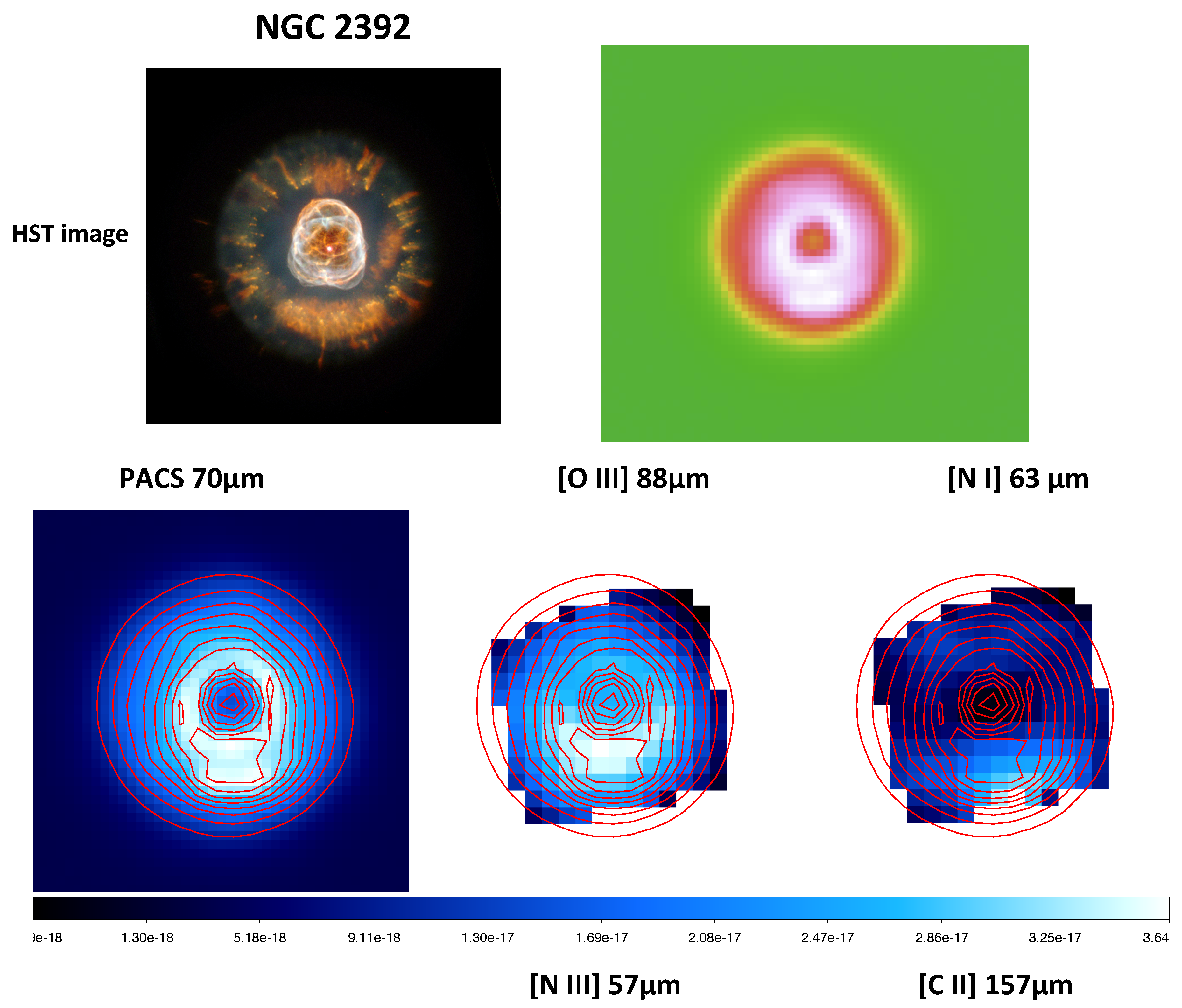
The HerPlaNS PACS spectroscopy observations consisted of mapping observations in selected emission lines for some PNe, and pointed observations covering the full spectral range for all the PNe. The first useful data product to create are therefore emission-line maps for all targets. We used the projected or interpolated cubes for the mapping observations, and the interpolated or rebinned cubes for the pointed observations. The maps were made by fitting a Gaussian profile to the emission line and a low-order polynomial to the continuum, over the entire cube, and then summing up the area of the fitted Gaussian. For the bright lines, where the slightly non-Gaussian nature of the PACS instrumental profile is more obvious (in the form of low-level broadened wings), we instead integrated under the emission line after having subtracted a low-order fit to the continuum: this recovers a few per cent of the total flux that the fitting misses. In both cases, the resulting maps are in units of integrated flux (W/m${}^2$) in each pixel, with the pixels being the same size as the spaxels of the cube used. Some example maps are shown in Figure 1, Figure 2 and Figure 3. In these figures, the IR images trace the thermal dust continuum, while the PACS spectral maps trace the gas. This spatial resolution in the PACS photometer images is ∼6${}^{″}$, with pixels of 3${}^{″}$, and in the spectrometer images is ∼9${}^{″}$, with pixels of 3${}^{″}$. Optical images are also shown for each PN, for comparison.

NGC 2392 is shown in Figure 1. The IR image at 70 $\mathsf{\mu }$m is of about the same size as the optical image. The PACS image shows the dust in the nebula, while the HST image (WFPC2, taken from the HST’s Hubblesite) is a composite of emission lines (H$\alpha$, He ii, [O iii], and [N ii]) and hence mostly gaseous emission. Two general morphologies in the PACS emission lines are seen: one seen in [N i] and [C ii] and the other in [N iii] and [O iii]. While both sets of ions peak in the south (where the optical and IR photometry do also), the region of highest surface brightness for the multiply ionised ions lies inside that of the singly ionised ions/atomic lines: at a first guess, this indicates a gradient in temperature.

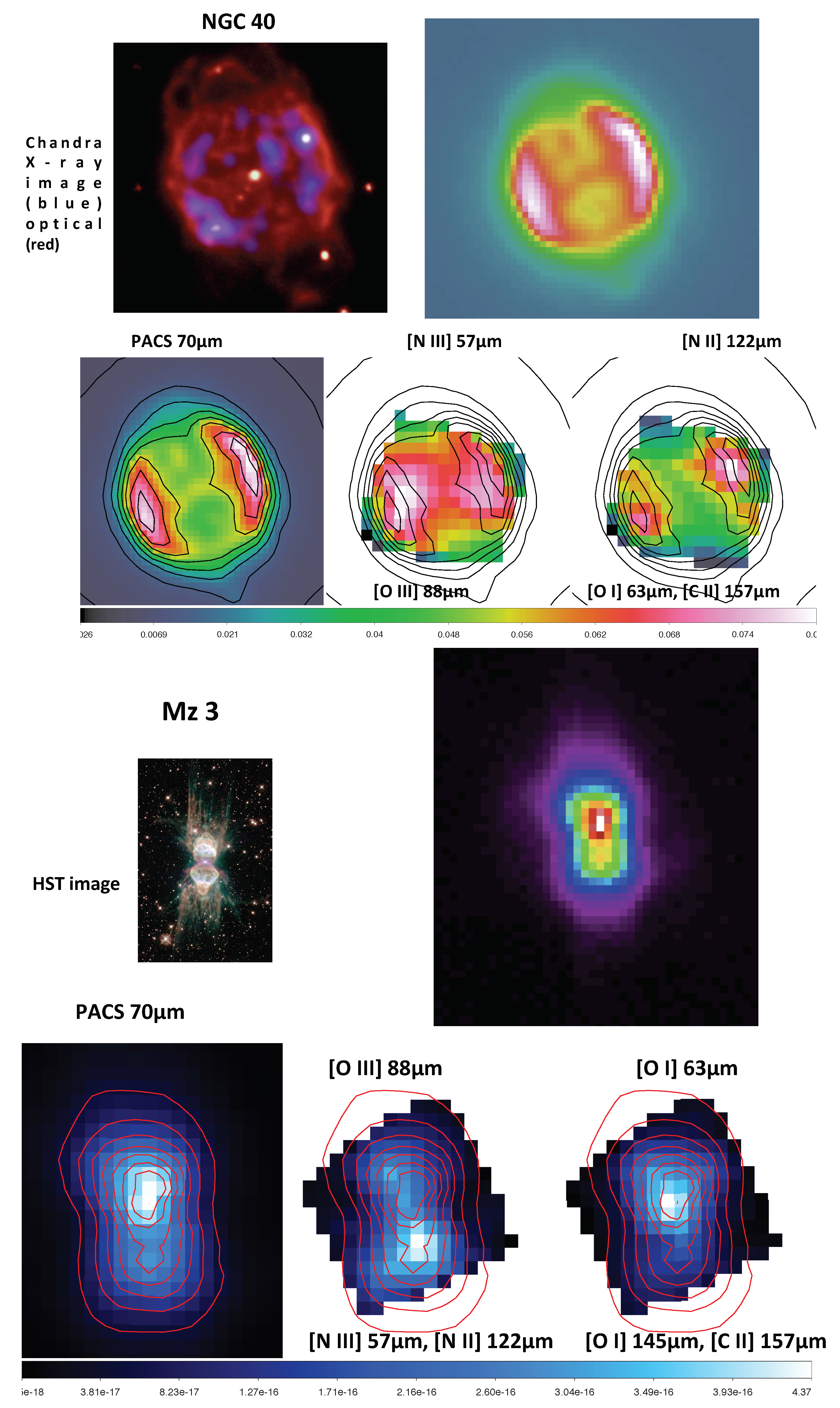
NGC 40 is shown in Figure 2. This nebula is described has a cylindrical or barrel-like shape in the IR. The X-ray/optical image composite (taken from the Chandra “photo album” website) and IR images in Figure 2 shows a similar E–W edge brightening. The X-ray image traces hot gas, suggested to result from the fast wind of the central star (Kastner et al. [5]), and it appears that this is delimited by the brightest parts of the dust in the nebula (i.e., the brightest parts of the PACS image). The IR emission lines also peak in these portions of the nebula. The peak of the multiply ionised ions ([N iiI] and [O iii]) is again differently-located to the singly-ionised ions/atomic line, however here they could be said to be slightly circularly rotated with respect to each other.

MZ 3 is shown in Figure 2. The optical image (WFPC2, taken from the HST’s Hubblesite) is a composite of emission lines (H$\alpha$, He ii, [S ii], and [N ii]) and hence mostly gaseous emission. The PACS photometer image (which is dust emission) shows a similar shape—the centrally-bright part of the IR image is about the same size as the optical image—but additional fainter emission can be clearly seen outside of this region (note that even PACS image is nicely resolved, and so this difference is not due to the different instrument resolutions). The surface brightness peak in the 70 $\mathsf{\mu }$m image is to the north, while the gas-tracing spectral lines peak in the centre (singly ionised ions/atomic lines) and south (multiply-ionised ions). This object certainly merits a closer inspection. Aleman et al. [3] reported on the detection of Hydrogen recombination laser lines in the PACS and SPIRE spectra of Mz 3.

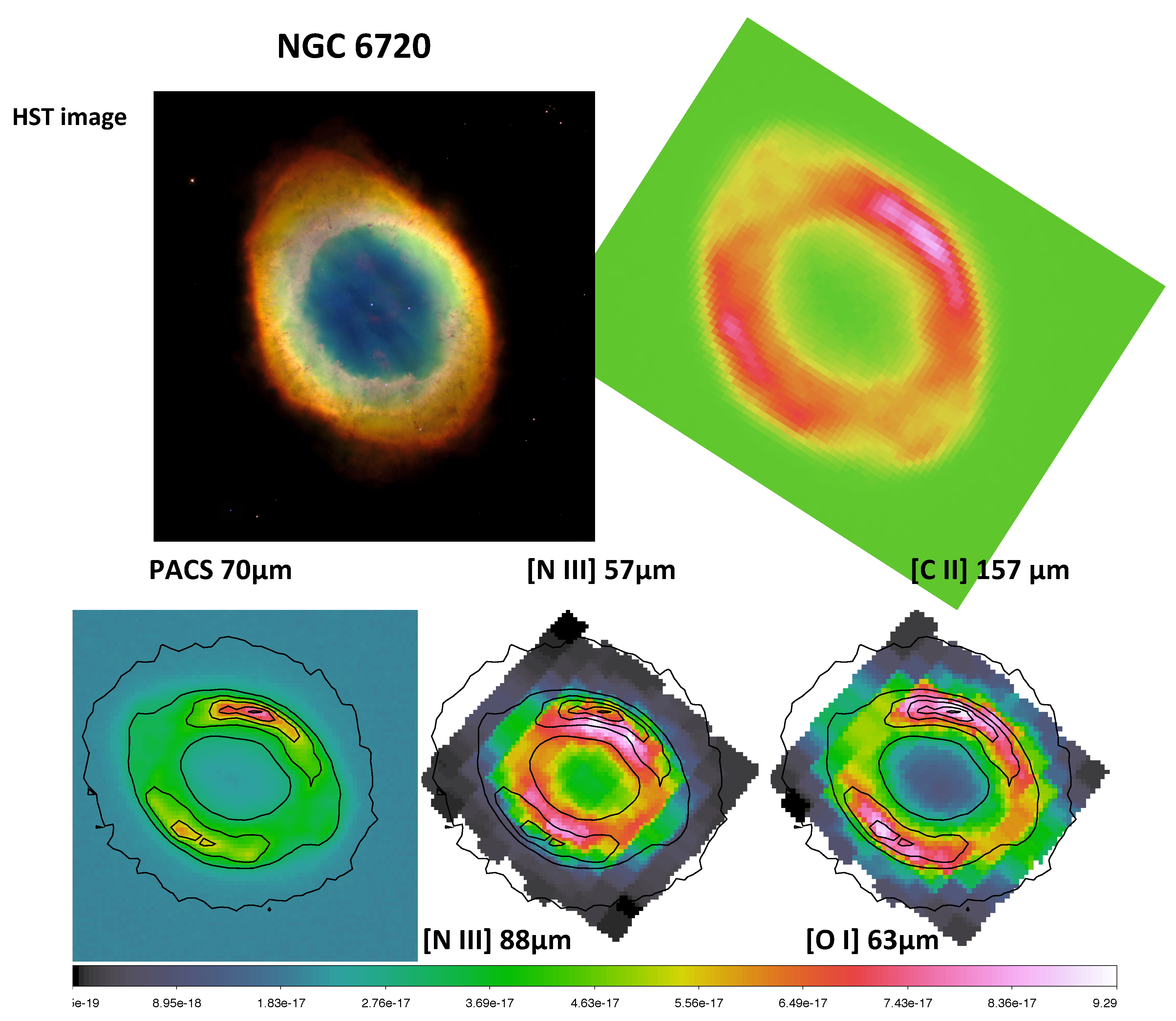
NGC 6720 is the final PN shown here, in Figure 3. This nebula has a very similar ring-like appearance in the optical (WFPC2, taken from the HST’s Hubblesite; is a composite of He ii, [O iii], and [N ii])) and PACS images. This ring-like appearance is the result of the projection of bipolar lobes pointing almost along the observer’s axis (e.g., O’Dell et al. [6]). The dust (measured from the IR photometry images) and gas (measured from the IR emission-line images) peak in the same location in the ring. It is clear that the surface brightness gradient is different between the multiply- and singly-ionised ions in the ring, pointing to a globally smooth variation in the physical conditions. NGC 6720 was included in the Herschel MESS programme (Groenewegen, et al. [7]), and PACS photometric data were used to study the knots in the ring (van Hoof et al. [8]).

4. Conclusions

Overall, we see a high degree of similarity between the the PACS photometer and spectrometer maps. However, the devil lies in the details: different ions peak at different locations in the nebulae, and this clearly will lead to information about the physical conditions and the structure of the nebulae. With such clear spatial variations, it is obvious that you do need to study the PNe in two dimensions.

A more careful comparison of the spectral maps to each other and to the photometer maps requires the additional step of matching the beam sizes at the different wavelengths, i.e., convolving the data to the same beam size.

We also need to consider the flux calibration more carefully. PACS cubes (and the spectral maps made from the cubes) are calibrated assuming the source is flat and extended, and for any other source morphology the flux calibration is not quite correct (this is documented on the PACS Overview page on the Herschel website). An attempt can be made to adjust the calibration to account for the unique source shape and observing (pointing) pattern of any target/observation. A script to do just this is provided on the HSC PACS pages and this is something that should be attempted for these sources.

References

- Ueta, T.; Ladjal, D.; Exter, K.; Otsuka, M.; Szczerba, R.; Siódmiak, N.; Aleman, I.; van Hoof, P.A.; Kastner, J.H.; Montez, R.; et al. The Herschel Planetary Nebula Survey (HerPlaNS)-I. Data overview and analysis demonstration with NGC 6781. Astron. Astrophys. 2014, 565, A36. [Google Scholar] [CrossRef]
- Aleman, I.; Ueta, T.; Ladjal, D.; Exter, K.M.; Kastner, J.H.; Montez, R.; Tielens, A.G.; Chu, Y.H.; Izumiura, H.; McDonald, I.; et al. Herschel Planetary Nebula Survey (HerPlaNS). First detection of OH+ in planetary nebulae. Astron. Astrophys. 2014, 566, A79. [Google Scholar] [CrossRef]
- Aleman, I.; Exter, K.; Ueta., T.; Walton, S.; Tielens, A.G.; Zijlstra, A.; Montez, R., Jr.; Abraham, Z.; Otsuka, M.; Beaklini, P.P.; et al. Herschel Planetary Nebula Survey (HerPlaNS): Hydrogen Recombination Laser Lines in Mz 3. Mon. Not. R. Astron. Soc. 2018, 47, 4499–4510. [Google Scholar] [CrossRef]
- Otsuka, M.; Ueta, T.; van Hoof, P.A.; Sahai, R.; Aleman, I.; Zijlstra, A.A.; Chu, Y.H.; Villaver, E.; Leal-Ferreira, M.L.; Kastner, J.; et al. The Herschel Planetary Nebula Survey (HerPlaNS): A Comprehensive Dusty Photoionization Model of NGC6781. Astrophys. J. Suppl. Ser. 2017, 231, 22. [Google Scholar] [CrossRef] [PubMed] [Green Version]
- Kastner, J.H.; Montez, R.; De Marco, O.; Soker, N. X-ray Imaging of Planetary Nebulae with Wolf-Rayet-type Central Stars. Bull. Am. Astron. Soc. 2005, 37, 437. [Google Scholar]
- O’Dell, C.R.; Ferland, G.J.; Henney, W.J.; Peimbert, M. Studies of NGC 6720 with Calibrated HST/WFC3 emission-Line Filter Images. I. Structure and Evolution. Astron. J. 2013, 145, 92. [Google Scholar] [CrossRef]
- Groenewegen, M.A.; Waelkens, C.; Barlow, M.J.; Kerschbaum, F.; Garcia-Lario, P.; Cernicharo, J.; Blommaert, J.A.; Bouwman, J.; Cohen, M.; Cox, N.; et al. MESS (Mass-loss of Evolved StarS), a Herschel key program. Astron. Astrophys. 2011, 526, A162. [Google Scholar] [CrossRef]
- Van Hoof, P.A.M.; Barlow, M.J.; Van de Steene, G.C.; Exter, K.M.; Wesson, R.; Ottensamer, R.; Lim, T.L.; Sibthorpe, B.; Matsuura, M.; Ueta, T.; et al. Herschel observations of PNe in the MESS key program. In Proceedings of the IAU Symposium 283: Planetary Nebulae: An Eye to the Future, Canary Islands, Spain, 25–29 July 2012. [Google Scholar]
Figure 1.
Images of selected PNe of the HerPlaNs programme. In all figures, the top shows an optical image for comparison to the PACS IR image at 70 m, these being approximately similarly scaled (N up, E left). The IR image is shown again on the bottom with contours to help the eye pick out the shape. These contours are then overplotted on two spectral images, which were chosen to demonstrate the morphology of the nebula in the indicated ions. The mapped ion identifications are printed above the spectral images, and those ions with a similar appearance are printed below. NGC 2392. (Top) An optical image (HST, WFPC2) and the PACS 70 m image. (Bottom) The PACS photometer image and two spectral images.
Figure 2.
(Top) NGC 40, with an X-ray/optical image composite and the PACS 70 m image, and the IR image with the two spectral images on the bottom. (Bottom) Mz 3, optical image (HST, WFPC2) and the PACS 70 m image at the top, and the IR image with the two spectral images on the bottom.
Figure 3.
NGC 6720, optical image (HST, WFPC2) and the PACS 70 m image at the top, and the IR image with the two spectral images on the bottom.
© 2018 by the author. Licensee MDPI, Basel, Switzerland. This article is an open access article distributed under the terms and conditions of the Creative Commons Attribution (CC BY) license (http://creativecommons.org/licenses/by/4.0/).
Share and Cite
MDPI and ACS Style
Exter, K. Spectroscopy of Planetary Nebulae with Herschel: A Beginners Guide. Galaxies 2018, 6, 73. https://doi.org/10.3390/galaxies6030073
AMA Style
Exter K. Spectroscopy of Planetary Nebulae with Herschel: A Beginners Guide. Galaxies. 2018; 6(3):73. https://doi.org/10.3390/galaxies6030073
Chicago/Turabian StyleExter, Katrina. 2018. "Spectroscopy of Planetary Nebulae with Herschel: A Beginners Guide" Galaxies 6, no. 3: 73. https://doi.org/10.3390/galaxies6030073
Note that from the first issue of 2016, this journal uses article numbers instead of page numbers. See further details here.