
Full Dynamic Ball Bearing Model with Elastic Outer Ring for High Speed Applications

Chair of Applied Mechanics, Technical University of Munich, 85748 Garching, Germany
*
Author to whom correspondence should be addressed.
†
These authors contributed equally to this work.
Lubricants 2017, 5(2), 17; https://doi.org/10.3390/lubricants5020017
Submission received: 30 April 2017
/
Revised: 2 June 2017
/
Accepted: 3 June 2017
/
Published: 12 June 2017
(This article belongs to the Special Issue Bearings in Turbomachinery)
Abstract
:Ball bearings are commonly used in high speed turbomachinery and have a critical influence on the rotordynamic behavior. Therefore, a simulation model of the bearing to predict the dynamic influence is essential. The presented model is a further step to develop an accurate and efficient characterization of the ball bearing’s rotor dynamic parameters such as stiffness and deflections as well as vibrational excitations induced by the discrete rolling elements. To make it applicable to high speed turbomachinery, the model considers centrifugal forces, gyroscopic effects and ball spinning. The consideration of an elastic outer ring makes the bearing model suitable for integrated lightweight bearing constructions used in modern aircraft turbines. In order to include transient rotordynamic behavior, the model is built as a full dynamic multibody simulation with time integration. To investigate the influence of the elasticity of the outer ring, a comparison with a rigid formulation for several rotational speeds and loads is presented.
1. Introduction
Widely used in common machinery, rolling element bearings permit a rotational motion between two components. The advantages of ball bearings like low friction and maintenance make them suitable for most applications. In contrast to journal bearings, no rotor instability occurs, which makes them perfect for high speed applications. The trend towards more powerful and lightweight turbomachinery requires precise control and prediction of rotor vibrations and dynamic behavior. A precise bearing model is essential for the following two reasons: first, it allows the calculation of typical rotordynamic coefficients like speed and load-dependent stiffness. These parameters are important for the determination of the rotor’s critical speeds as well as for the definition of the operational ranges. Second, a precise bearing model provides insight into the bearings excitation frequency. For instance, under radial load, there is always an excitation in the range of the ball passing frequency due to the discrete rolling elements. A damaged bearing with faults at the raceways or the balls generates additional system excitations in frequency ranges, which can be calculated in the dynamic simulation. In high speed lightweight applications such as turbopumps or compressors, angular contact ball bearings are used. They are axially preloaded to avoid clearance. The associated ball kinematics cause, besides the centrifugal forces, gyroscopic moments and ball spinning. This causes additional loads and wear that have to be considered in machinery design. In lightweight turbomachinery, mostly for highly integrated aircraft applications, the bearing raceways are directly integrated in the shaft and the housing itself. This hinders the direct prediction of the bearing effects on the rotordynamics. To follow this aspect in this contribution, the outer bearing ring is modeled elastically using the finite element method (FEM). This allows the determination of the interaction between the balls and the elastic structure resulting in overall shaft support stiffness.
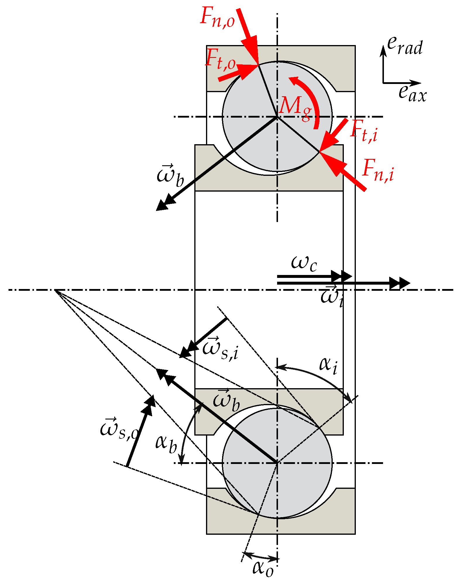
The issue of bearing modeling has been dealt with for over 50 years. Among the first who dealt deeper with kinematic and kinetic analyzes were Jones [1] and Harris [2]. Due to the lack of computing power, no extensive dynamic simulations could be carried out, which led to a quasi-static model with many simplifications. Firstly, the geometric relationships and quantities within the bearing were outlined by Harris. Secondly, contact forces and deformations (see Figure 1) were derived based on the Hertzian-contact theory.
Using the simplification stated by the race control hypothesis, which assumes that there is no relative motion between the ball and the bearing rings surface ( and ) and the inclusion of centrifugal forces and gyroscopic moments , equilibrium relationships were derived. Further simplifications are made by neglecting the ball–cage interaction and assuming identical angular distribution of the balls around the rotation axis of the bearing.
The model of Koch [3] and later Tüllmann [4] is an extension of Harris’ study. The aim of this work was the investigation of increased maximum speed for axially loaded angular contact ball bearings. They extended the modeling by a degree of rotational freedom for the cage, rotating around the center of the outer ring.
To compute the angular velocity of the balls , they first determine the angle by geometric relations, assuming pure rolling on both raceways. The different contact angles between the ball and the raceway ( and ) cause a relative rotational movement between the surfaces (spinning motion) . Using a friction model of the elastohydrodynamic (EHD) theory, a spinning friction loss results as a function of the ball rotating angle . By minimizing the power loss, the required rotating angle is calculated. The gyroscopic moment can then be determined by the ball rotation and the angle . This is taken into account as a tangential force at the contact point in the force equilibrium of the inner and outer ring (Figure 1).
Another approach to investigate the dynamic bearing behavior is made by Oest [5] and later Fritz [6]. They describe the rotational speed of the balls and the cage in the assembly purely from geometrical considerations in the static, unloaded position. This is possible assuming an equal ball contact angle on the inner and the outer ring. Simplifications are also made by neglecting the gyroscopic moments, the centrifugal forces, and the drilling friction forces of the balls. These assumptions are made under the condition of pure rolling at low operation speed.
A very detailed model for rolling bearings is the ADORE program developed by Gupta [7] over decades. It describes the behavior of the bearing through a quasi-static as well as a dynamic model. With the static model, starting solutions for the dynamic simulation are determined with assumptions similar to Koch’s (no cage interaction, calculation of the ball rotation via a race control assumption under kinematic relations). The dynamic model does not require any kinematic relationships or geometric assumptions and describes both roller skidding and skewing as well as the lubricating film behavior. For this purpose, six degrees of freedom (DOF) per bearing component are used, which are coupled through the forces.
Another model is the BEAST program developed by Stacke and Fritzson [8] for the company SKF (Gothenburg, Sweden). As the model of Gupta, each bearing component has six degrees of freedom, but the contact forces between the cage and the rolling elements are described in more detail. This allows for computing additional effects numerically, such as the power loss, the lubrication film behavior as well as the forces on the cage and its behavior.
To study the bearings’ vibrational behavior, Sassi [9] presents a 1D model limited to 3 DOF (both rings and one ball) to study the dynamic response of a localized defect in the bearing. Another more detailed approach is made by Tkachuk [10], who uses a 3D dynamic model with 4 DOF for each part of the bearing. They analyze the effect of axial load and misalignment on the vibration signal.
Tadina [11] uses a bearing simulation model with finite element housing to simulate the vibrational response of the bearing to different local faults, modeled as ellipsoids on the races. Modeling the raceway faults or imperfections with sinusoidal functions is proposed in [12].
To determine the effects of a varying ball number and centrifugal forces on the dynamic response and excitation of the rotor system, Vakharia [13] developed a simulation model that includes specific geometric constraint assumptions for the cage speed and the ball positions.
The description of the lubricant’s behavior, the friction model as well as the EHD damping effects can require time-consuming computations. However, Wijnant [14] presents an alternative approximation method for lubricated contacts in order to gain computing efficiency and keep an acceptable level of accuracy for the EHD contact loads and damping coefficients [15]. For instance, in the frame of a rotor dynamic study, the outer ring as well as the housing and the shaft can be modeled as flexible bodies using finite element techniques including a modal reduction [14,15].
Another method consists of a multi-level model, which interpolates the solution from a set of precomputed values to provide faster results for EHD computations (see [8,16]).
The motivation for the authors’ work is to develop a fast dynamic simulation model, which includes all relevant effects for high speed applications. Therefore, a minimal set of degrees of freedom, analytical and physical motivated solutions are used to avoid the most kinematic and kinetic simplifications. Besides the classic rigid bearing model, the elasticity of the outer ring is included.
The structure of this paper is as follows: in Section 2, the kinematics of the bearing components and the dominating forces are described. Section 3 outlines the modeling of the elastic outer bearing ring including a reduction of the full finite element model of the ring. The full dynamic model is summarized in Section 4 and the time integration scheme is outlined. Section 5 gives a case study of a bearing simulation and analyzes the influence of the elasticity of the outer ring on the rotordynamic coefficients and the vibrational behavior. In Section 6, conclusions are drawn.
2. Bearing Kinematics and Forces
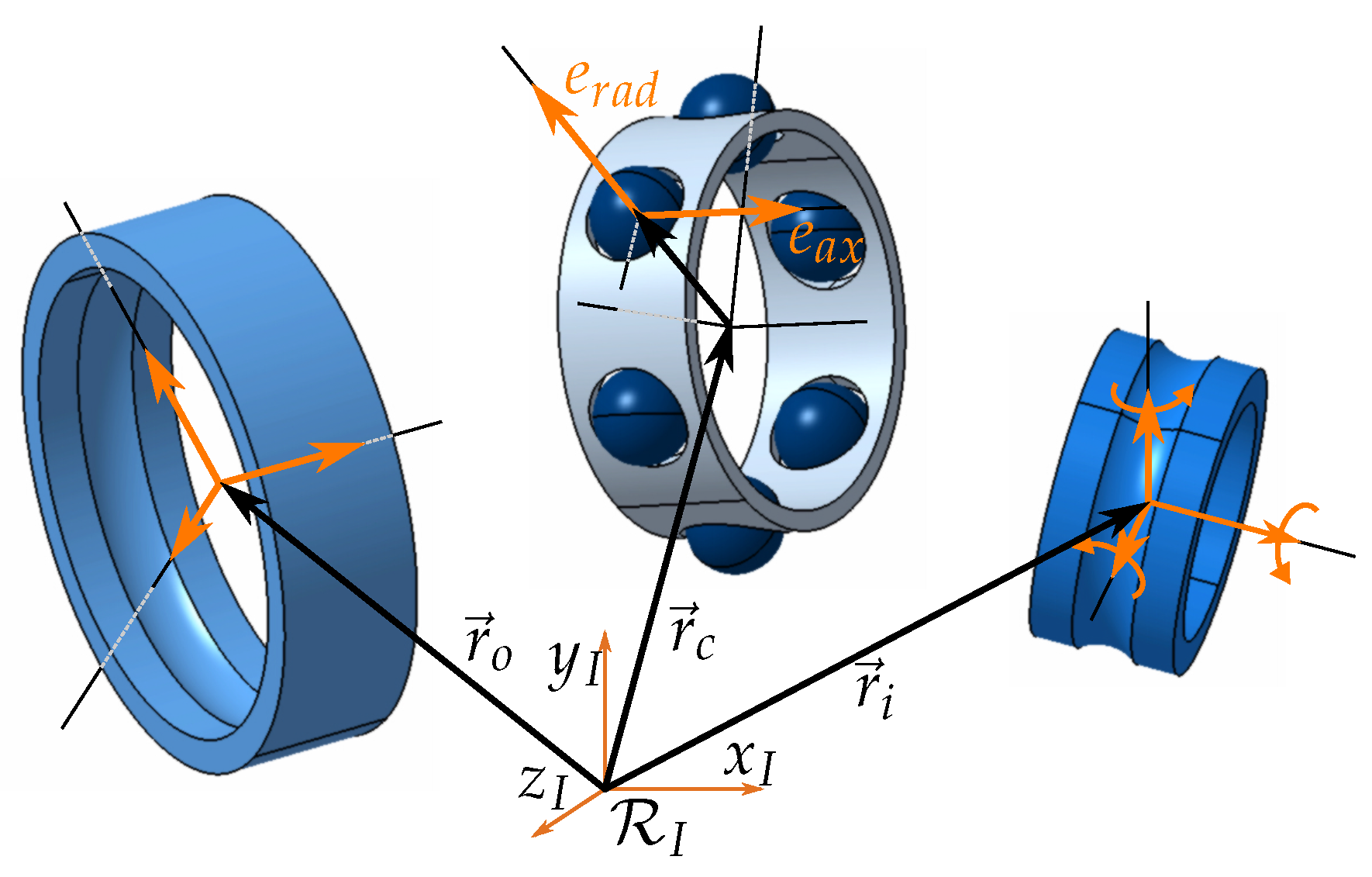
The presented angular contact ball bearing model is based on a multibody simulation, using 6 DOF for the inner ring, 2 DOF for each ball (their axial and radial displacements) and 250 DOF for the elastic outer ring. The coordinate frames used to describe the bearing configuration are shown in Figure 2.
The origin of the inertial coordinate system is fixed at the center of the outer ring, so that . In order to describe the balls’ positions, the local coordinate frame () is used. Each ball’s local system is established according to the angle and determined by the cage rotation .
To describe the ball-inner race and ball-outer race contacts and interactions, local coordinate frames () and () are used (see Figure 3). and represent the balls’ degrees of freedom.
2.1. Deflections, Normal Forces and Cage Speed
The main step to describe the bearing behavior is to calculate the contact deflections and as well as the contact angles and between the ball and the inner and outer raceway (Figure 3). Therefore, a detailed description of the inner bearing geometry and geometric projections of the degrees of freedom are used. In the general bearing configuration, the contact angles are different between inner and outer ring because of the acting centrifugal forces. This is taken into account by using the 2 DOF of each ball and can be calculated with the dynamic equilibrium.
Assuming a pure rolling condition, meaning no slip in circumferential direction, the velocities of the ball centers can be calculated (see Figure 4):
and the ball rotation is given by
with the ball contact positions and , respectively, and the velocity parts in circumferential direction and .
Since each ball can be positioned differently in the rings, depending on the contact geometry and the ring positions, the velocity of the ball contact point can differ in addition to the velocities of the center of the balls. However, the cage constrains them all to a prescribed velocity determined by the rotational velocity of the cage. To calculate the resulting rotational velocity , different methods exist. Here, in this contribution, a method based on a weighting approach is used and presented in the following.
The first step is to calculate the ball normal Hertzian contact forces and using the deflections and (see, for instance, [6]:
with the Hertzian stiffness coefficient (see [5]). Note that, in this present study, the effect of lubrication is neglected. Its influence may require further investigations and could be considered, for instance, by a contact force law as derived by Wijnant [14].
The improved method to calculate the cage speed is to take a weighted mean of the ball center velocities with the normal contact forces as weighting factors (see Figure 4):
with
using k for the ball number. This weighting approach ensures that the velocities of balls, which are highly loaded, are taken more into account than the velocities of balls, which are not loaded. Therefore, the higher the force , the more a ball is considered to satisfy the pure rolling condition. If a ball has no contact, an unloaded clearance zone occurs and no forces act on the cage. As the gyroscopic moments counterbalancing tangential forces are acting perpendicular to the cage rotation speed, they are not taken into account in this weighted averaging.
Having the cage speed , the centrifugal forces acting on the balls are calculated with the ball mass and the difference of and :
They are acting in the direction of .
2.1.1. Spinning, Skidding and Gyroscopic Moments
To calculate the gyroscopic effects of the rolling elements, the balls’ rotational velocity is needed. The ball rotation axis cannot be normal for both contact ellipses at the outer and inner ring contacts simultaneously because of the different angles and . This causes relative rotation velocity at the contact points, called here spinning motion and denoted by and at the raceways (see Figure 4). It generates the power loss and wear on the surfaces due to the friction forces at the contact ellipse. The determination of the ball rotation is not possible using only geometrical constraints.
A modern approach for this calculation of is made by [3,4]. It is applied to every ball in this dynamic bearing model. The methodology is to minimize the ball spinning power loss to get the ball’s rotation angle . Therefore, the ball spinning motion for each contact is calculated depending on the ball rotation vector: . The power loss is then calculated using the spin vector and the relative skidding velocity to:
where is the slip velocity and is the friction shear stress in the contact ellipse at point P, the integration taking place over the entire ellipse (see Figure 5). The chosen dry coulomb friction coefficient for steel is and is the local hertz pressure. The local slip velocity at point P is:
The skidding velocity is calculated from the cage rotation and the contact point velocities assuming that the skidding velocity at both contact points is equal (), so:
The calculated power loss is then added for both contacts for each ball and is a function of the ball rotation vector and its angle and magnitude. A numerical minimization of the power loss leads to and must be performed in each timestep. The reached power loss and the spinning motion are a part of the whole bearing losses and can be used for frictional, thermal or wear calculations.
The gyroscopic moments caused by the misalignment between the balls’ rotation and the bearing axis are shown in Figure 1. It is defined with the balls’ moment of inertia as:
We assume that these gyroscopic moments are in equilibrium with the moments created on the ball by the tangential forces (Figure 1), acting at the ball-race contact points.
2.1.2. Damping in Ball Race Contact
In our dry bearing case, there is only little damping compared to the lubricated one, where the elastohydrodynamic oil film generates the damping forces. However, the cyclic deformation of a linear-elastic material causes energy losses that correspond to the hysteresis on a load-displacement diagram. For a specific material, the loss factor corresponds to the dissipated energy and the strain energy over a deformation cycle (see [5]):
For this model, is chosen for each bearing contact. To propose a viscous damping coefficient c, the energy dissipation is compared for a 1D oscillator system. The resulting coefficient c is a function of , the Hertzian contact stiffness and the deformation frequency , the ball passing frequency ( is the number of balls), to [5]:
3. Modeling of the Elastic Outer Ring
So far, the local penetration between ball and outer raceway is taken into account due to the Hertzian contact model (see Section 2.1). In order to cover the global deflection of the outer raceway in addition to the local one, an elastic model for the bearing outer ring is considered. The inner ring elasticity can also be modeled. As an example, only the elasticity of the outer ring is considered. In this work, it is represented by a reduced finite element model with linear elastic material behavior.
The following steps describe representatively the process of the outer ring modeling. First, the physical dimensions define the geometry of the elastic ring. Second, a discretization by the finite element method gives the governing equations for the full outer ring model. In the last step, an adequate reduction method decreases the size of the full model for a later efficient consideration in the dynamic simulation. Here, the Craig–Bampton approach is applied.
3.1. Geometry
The geometry of the bearing outer ring is defined by the physical dimensions of the rigid bearing. As an example, without loss of generality, the outer ring is approximated in the following by a cuboid of dimensions with the side length and the width of the outer ring. The cuboid has a hollow cylinder with diameter representing the outer raceway inside the bearing ring. Despite the simple FE geometry, the detailed geometric curvature of the outer raceway is still considered by an analytical superposition. Thus, it is possible to choose a very crude or highly reduced FE mesh and to represent a real bearing raceway geometry (represented by the curvature radii and its centers) for calculating the deflections and contact forces.
3.2. Finite Element Approach
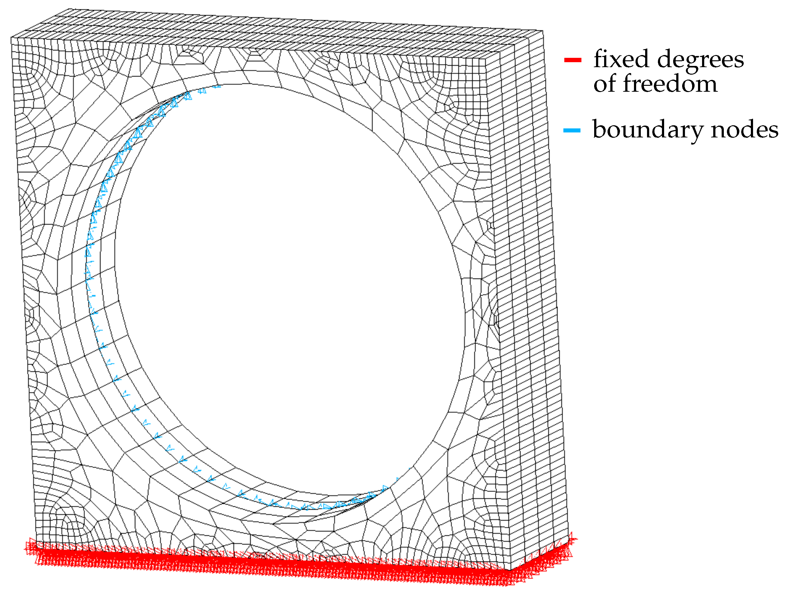
In the next step, a finite element approach is used in order to discretize the structural equations of the bearing ring. This step is performed in a finite element software tool. The elastic volume is discretized by using three-dimensional incomplete quadrilateral elements (each with 20 nodes) with serendipity shape functions. A structured mesh is applied to the interface of the hollow cylinder by using 40 elements in circumferential and four elements in axial directions, respectively. Bi-quadratic finite elements (each with eight nodes) are used for the interface. The degrees of freedom of the nodes of the cuboid’s bottom are fixed. Figure 6 shows the finite element model of the bearing outer ring structure. The homogeneous space-discretized equation of the full finite element model is stated as
with the finite element mass matrix and the finite element stiffness matrix . The vector represents the N elastic coordinates of the full ring model.
3.3. Reduction Methodology
Due to the large number of elastic degrees of freedom, the full finite element model can hardly be handled in a dynamic multibody simulation. Therefore, in the following, the full model with its N degrees of freedom is reduced by the classical Craig–Bampton method.
For the Craig–Bampton reduction, the vector of the full model is decomposed into a vector containing displacements of boundary nodes and a vector containing displacements of inner nodes. The degrees of freedom are thus partitioned as with the total number of nodes . As the boundary nodes are later retained for the reduced model, they are chosen as the nodes that belong to the circle of the outer raceway, indicated in blue in Figure 6. The residual nodes correspond to the inner nodes of the model. Then, a reduction by the Craig–Bampton approach is defined as:
The first columns of the reduction basis T are interface constraint modes based on unit displacements of the boundary coordinates . The remaining columns contained in the matrix a set of fixed interface normal modes. They are determined by restraining all boundary nodes and solving the obtained eigenvalue problem for the first eigenvalues. Using the reduction of Equation (14), the following reduced mass and stiffness matrices are obtained:
In the later example, 80 boundary nodes and hence constraint modes and vibration modes are used.
It is noteworthy that other approaches could also be used for the reduction of the full outer ring structure model. For instance, the already reduced model could be further reduced by a modal truncation approach, as followed by Novotny [17] for elastic journal bearings. In addition, a load dependent approach by using free interface normal modes and attachment modes could have been followed (see [18,19,20]).
4. Full Dynamic Bearing Model
The bearing assembly can be seen as two different parts: The bearing elements (the balls, cage and inner ring) and the elastic outer ring structure. The movements of the bearing elements lead to a multibody simulation, in which the elastic outer ring is a structural dynamics element.
The two parts are coupled using projections of the displacements and forces with interpolations to the constraint modes. This is discussed in detail next.
4.1. Multibody Simulation
Modeling the bearing components, the kinematics and kinetics lead to a dynamic equilibrium for each bearing component. For the inner ring, the dynamic equation writes:
where is the vector of external forces on the inner ring. For the dynamic equation of motion of each ball k follows, using :
where the matrix transforms the ball forces into the local ball coordinate system. The centrifugal forces are summarized in the vector . The outer ring follows with , and the equation:
where the Jacobi matrix projects the k-th ball forces into the direction of the coordinates of the finite element model of the outer ring.
These three equations are summarized to a set of dynamic equations of motion of the whole bearing. A time integration scheme (MATLAB ode15s, R2016b, 7 September 2016, The MathWorks Inc., Natick, MA, USA) applied to the state space formulation of the system is used in order to get the component velocities and displacements over time.
4.2. Deflection Calculation
The contact deflection and of each ball on the inner and outer raceway, respectively, is calculated from the current state variables. The deflection depends on the coordinate vector of the inner raceway and the coordinate vector of the k-th ball. The deflection depends on the coordinate vector of the k-th ball and the current elastic deformation of the bearing housing at the ball angle (Figure 4), which is in the following denoted by . The latter deformation is interpolated from the deformation of the neighboring nodes by using the bi-quadratic shape functions used for the finite element discretization.
4.3. Force Projections
The ball forces , and , on the inner and outer raceway, respectively, are calculated on the basis of the local deflections (see Equation (3)). While they can be directly applied to the dynamic equations of the inner ring (see Equation (16)), they have to be transformed into the local coordinate system by a matrix , when applying them to the dynamic equation of the k-th ball (see Equation (18)). At the outer raceway, they have to be projected onto the elastic coordinates at the ball angle (Figure 4). Therefore, the Jacobi matrix is used (see Equation (18)). It contains the bi-quadratic shape functions used for the finite element discretization and evaluated at the current position .
4.4. Bearing Model Implementation
The coupling of the two parts is done directly by projecting the elastic housing’s deformation to the contact deflections of the outer raceway. The normal and tangential forces are then projected back from the raceway to the housing. In this way, it is possible to add the state space formulation of the housing directly to the bearing state vector. Thus, the overall dynamic equilibrium is solved for each timestep.
4.4.1. Outer Ring Structural Damping
To add damping to the elastic housing, two approaches are combined. The elastic housing modes are damped by modal damping using the modal expansion to build the viscous damping matrix (see [21]):
with for the generalized mass of the state space mode . is the mass matrix of the elastic housing with stiffness matrix .
The static degrees of freedom of the housing (viscous damping matrix ) are damped using the Rayleigh approach:
with . The whole damping matrix is then assembled:
To speed up the time integration scheme and to choose realistic initial conditions, the static equilibrium is solved beforehand.
5. Results of Representative Example
Showing the differences in the bearing behavior between a rigid and elastic outer ring formulation is the task of this chapter.
The examined ball bearing is a standard deep groove ball bearing of type 6404. Its outer diameter is 72 mm, the inner is 20 mm, and it includes six balls with a diameter of 15.1 mm. The material is steel and no lubrication is used. In the elastic housing case, the outer ring is replaced by the flexible structure. For a realistic rotor case simulation, some shaft mass (1 kg) and stiffness are added to the bearing’s inner ring, which leads to neglecting the rotation of the inner ring system around and .
The results should not necessarily represent a realistic bearing. Instead, they are presented to show the differences of the model methodology and the advantage of detailed elastic formulations.
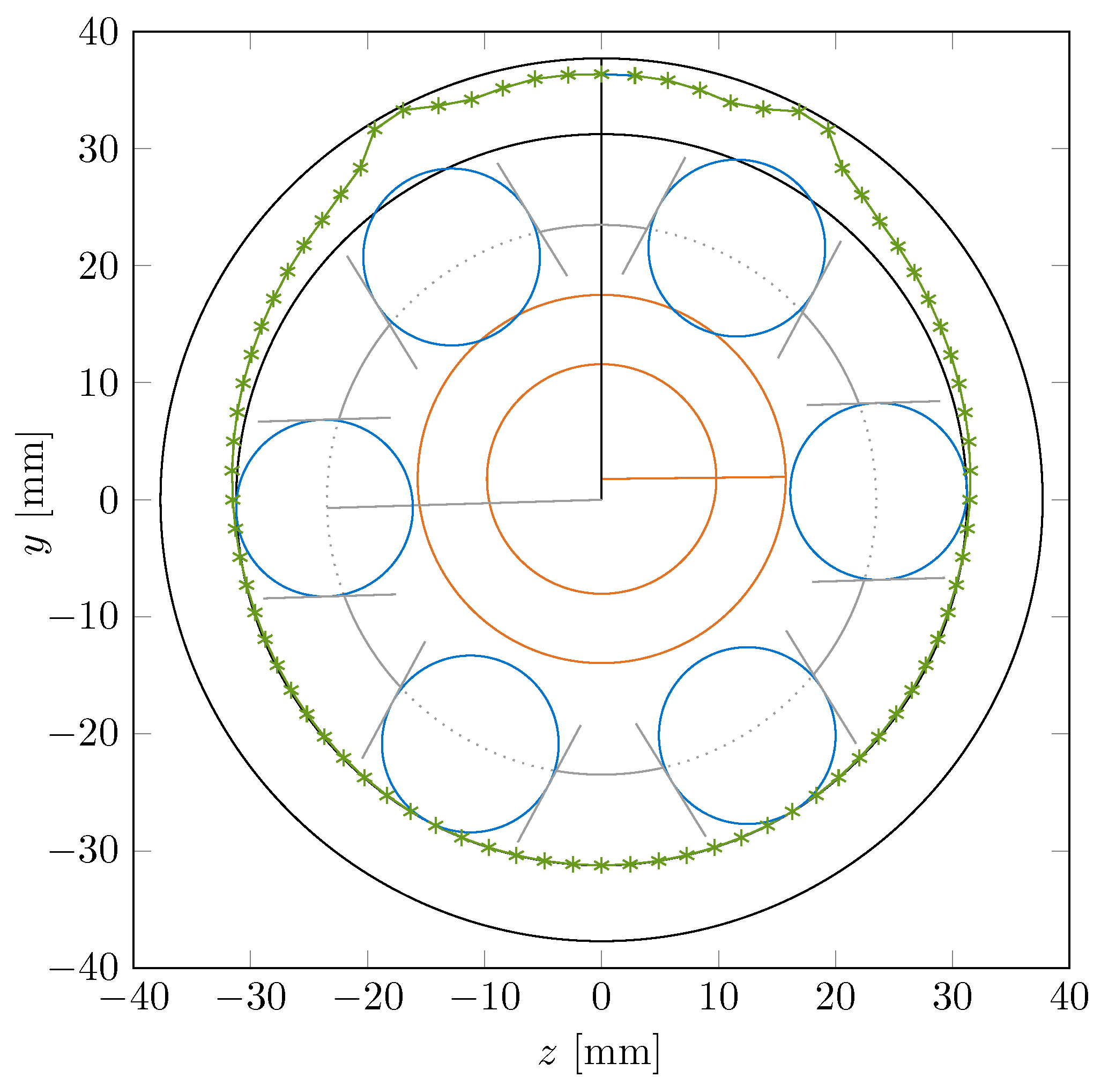
Figure 7 shows a snapshot of the dynamic simulation (time-dependent) of the bearing. It is loaded by a constant radial force of 1000 N in a positive y-direction (upwards in the figure). The shaft rotates at 1047 rpm. The green points represent the position of the elastic housing. It can be seen that the balls have a Hertzian deflection additionally to the housing’s deformation. The deflections and deformations are amplified for better visualization. In contrast to a homogeneous black box formulation, the inhomogeneous load distribution can be seen clearly.
5.1. Bearing Displacements
The radial inner ring displacements (shaft movement) are shown in Figure 8. The bearing is loaded with radial force, in the y-direction, at several rotational speeds (3000, 6000, 12,000, 24,000 rpm) for a rigid and elastic housing formulation.
Within the rigid configurations, the speed dependency is only minor. The centrifugal forces are small with regard to the Hertzian stiffness. In the elastic housing case, a larger influence of the rotational speed can be seen. The higher the shaft speed, the higher the radial displacement.
The absolute inner ring displacement of the elastic formulation is higher compared to the rigid one. This shows the weakening effect of a soft outer ring structure. Figure 9 shows the radial bearing stiffness calculated from the displacements.
5.2. Bearing Excitation Frequencies
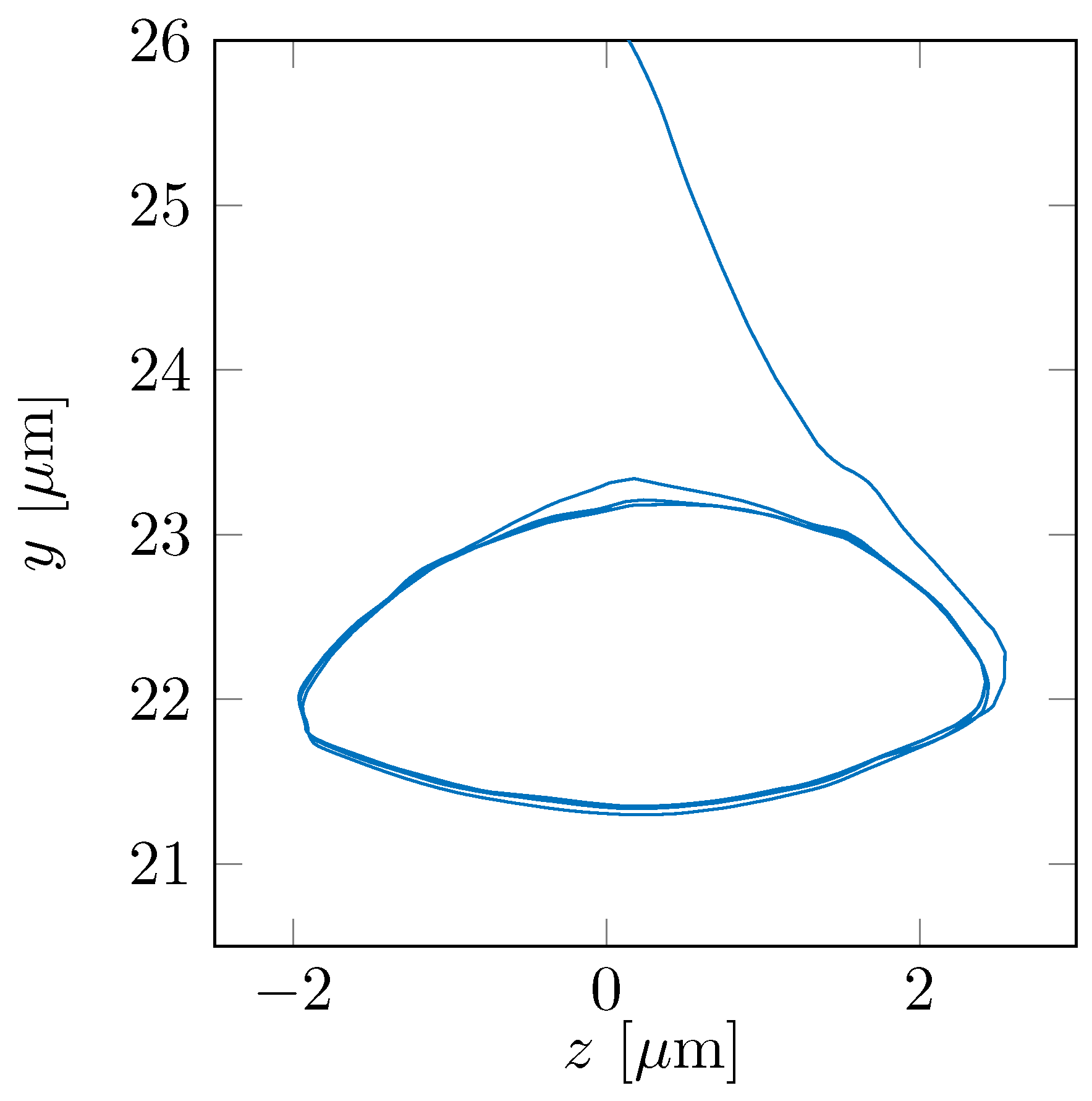
The consideration of the bearing as an inhomogeneous, discrete parted element leads to a rotating angle-dependent behavior. Depicted in Figure 10 is the orbit plot of the inner ring motion of the constant radial loaded bearing (1000 N) at a constant rotational speed of 1000 rpm.
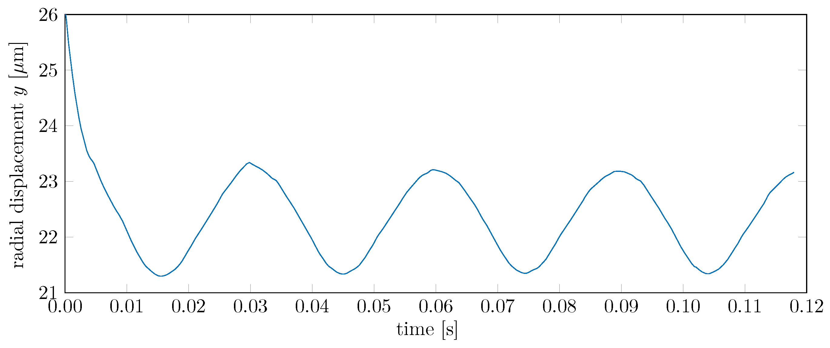
It indicates a movement of the shaft in an elliptic orbit. The center location is not constant unlike the load, so the dynamic simulation is useful to predict the amplitudes. The frequency of this orbit is described mainly by the ball passing frequency (see Figure 11). It has to be considered to avoid a rotor resonance at that frequency. In this case, the inner ring rotates at 1000 rpm, corresponding to 16.7 Hz.
The dominating excitation frequency is about 33.9 Hz. It excites higher frequencies of the elements and the housing. The ball passing frequency is determined by the cage speed and the number of balls. An accurate calculation, presented in this paper, is useful for the machinery design process.
6. Conclusions
In this paper, a full dynamic multibody bearing simulation including an elastic outer ring is presented. The discrete elements of the bearing, the inner ring, the balls and the cage are described. To calculate the acting forces, the Hertzian theory and deflections between the bearing elements are used. To model a bearing integrated into a lightweight structure, the bearing outer ring is modeled as an elastic structure using the FEM approach and reduction techniques. Projections of forces and displacements are used to couple the multibody simulation to the structural part. This formulation makes it possible to examine the ball–structure interaction and the whole dynamic bearing behavior. A time integration leads to the shaft and bearing elements dynamic motion. To compare the elastic and the rigid outer ring approach, some stiffness and displacement results are shown. The orbit movement can lead to a vibrational excitation of the rotor. The excitation frequency is calculated using a detailed physically motivated bearing cage approach. The model still contains simplifications like the assumption of constant radii for inner and outer raceway shapes, the neglect of cage inertia and clearance effects, the simplified FE geometry or the absence of lubrication. These simplifications give space for future investigations; for instance, the validation of the model by experimental data could provide deeper knowledge on the underlying effects.
Acknowledgments
This project is supported by the Ludwig Bölkow Campus and the Bavarian State. The good cooperation between the partners within the research project is well appreciated. In addition, this work was supported by the German Research Foundation (DFG) and the Technical University of Munich (TUM) in the framework of the Open Access Publishing Program.
Author Contributions
Christian Wagner and Andreas Krinner built up the simulation model. Christian Wagner analyzed the results and wrote the main part of the paper. Andreas Krinner wrote the section of the elastic formulation. Thomas Thümmel and Daniel Rixen added useful information and discussions relevant to this study.
Conflicts of Interest
The authors declare no conflict of interest.
References
- Jones, A.B. A General Theory for Elastically Constrained Ball and Radial Roller Bearings Under Arbitrary Load and Speed Conditions. J. Basic Eng. 1960, 82, 309–320. [Google Scholar] [CrossRef]
- Harris, T.A. Rolling Beasing Analysis, 3rd ed.; Wiley-Interscience: New York, NY, USA, 1991; p. 1013. [Google Scholar]
- Koch, A. Steigerung der Höchstdrehzahl von Schrägkugellagern bei Ölminimalmengenschmierung. Ph.D. Thesis, TU Aachen, Aachen, Germany, 1996. [Google Scholar]
- Tüllmann, U. Das Verhalten Axial Verspannter, Schnelldrehender Schrägkugellager. Ph.D. Thesis, TU Aachen, Aachen, Germany, 1999. [Google Scholar]
- Oest, H. Modellbildung, Simulation und Experimentelle Analyse der Dynamik Wälzgelagerter Rotoren. Ph.D. Thesis, Universität Rostock, Rostock, Germany, 2004. [Google Scholar]
- Fritz, F. Modellierung von Wälzlagern als Generische Maschinenelemente einer Mehrkörpersimulation. Ph.D. Thesis, Karlsruher Institut für Technologie, Karlsruhe, Germany, 2011. [Google Scholar]
- Gupta, P.K. Advanced Dynamics of Rolling Elements, 1st ed.; Springer: New York, NY, USA, 1984; p. 296. [Google Scholar]
- Stacke, L.E.; Fritzson, D. Dynamic behaviour of rolling bearings: Simulations and experiments. Proc. Inst. Mech. Eng. J 2001, 215, 499–508. [Google Scholar] [CrossRef]
- Sassi, S.; Badri, B.; Thomas, M. A numerical model to predict damaged bearing vibrations. J. Vib. Control 2007, 13, 1603–1628. [Google Scholar] [CrossRef]
- Tkachuk, P.A.; Strackeljan, J. Dreidimensionales dynamisches Wälzlagermodell für Schadenssimulation unter Variation von Kontaktbedingungen. J. Mech. Eng. Natl. Tech. Univ. Ukr. Kyiv Polytech. Inst. 2011, 1, 51–55. [Google Scholar]
- Tadina, M.; Boltežar, M. Improved model of a ball bearing for the simulation of vibration signals due to faults during run-up. J. Sound Vib. 2011, 330, 4287–4301. [Google Scholar] [CrossRef]
- Strackeljan, J.; Goreczka, S.; Doguer, T. Detection of bearing faults in high speed rotor systems. In Proceedings of the Ninth International Conference on Condition Monitoring and Machinery Failure Prevention Technologies, London, UK, 12–14 June 2012. [Google Scholar]
- Vakharia, V.; Gupta, V.; Kankar, P. Nonlinear Dynamic Analysis of Ball Bearings Due to Varying Number of Balls and Centrifugal Force. Mech. Mach. Sc. 2015, 21, 1103–1113. [Google Scholar]
- Wijnant, Y.H. Contact Dynamics in the Field of Elastohydrodynamic Lubrication. Ph.D. Thesis, University of Twente, Enschede, The Netherlands, 1998. [Google Scholar]
- Wensing, J.A. The Dynamics of Ball Bearings. Ph.D. Thesis, University of Twente, Enschede, The Netherlands, 1998. [Google Scholar]
- Bizarre, L.; Nonato de Paula, F.; Cavalca, K. EHD Modeling of Angular Contact Ball Element Bearings. In Proceedings of the 9th IFToMM International Conference on Rotor Dynamics Mechanisms and Machine Science; Springer International Publishing: Cham, Switzerland, 2015; Volume 21, pp. 1103–1113. [Google Scholar]
- Novotny, P.; Pistek, V. New efficient methods for powertrain vibration analysis. Proc. Inst. Mech. Eng. D 2010, 224, 611–629. [Google Scholar] [CrossRef]
- Géradin, M.; Rixen, D.J. A ‘nodeless’ dual superelement formulation for structural and multibody dynamics application to reduction of contact problems. Int. J. Numer. Methods Eng. 2015, 106, 773–798. [Google Scholar] [CrossRef]
- Krinner, A.; Rixen, D.J. Interface reduction methods for mechanical systems with elastohydrodynamic lubricated joints. In Proceedings of the 27th International Conference on Conference on Noise and Vibration Engineering (ISMA 2016), KU Leuven, Belgium, 19–21 September 2016. [Google Scholar]
- Fiszer, J.; Tamarozzi, T.; Desmet, W. A semi-analytic strategy for the system-level modelling of flexibly supported ball bearings. Meccanica 2016, 51, 1503–1532. [Google Scholar] [CrossRef]
- Geradin, M.; Rixen, D.J. Mechanical Vibrations: Theory and Application to Structural Dynamics, 3rd ed.; Wiley-Interscience: New York, NY, USA, 2015; p. 617. [Google Scholar]
Figure 1.
Ball bearing’s kinetics and kinematics.

Figure 2.
Degrees of freedom and coordinate systems.

Figure 3.
Local ball-race contact coordinate frames.

Figure 4.
Velocities in the ball bearing.
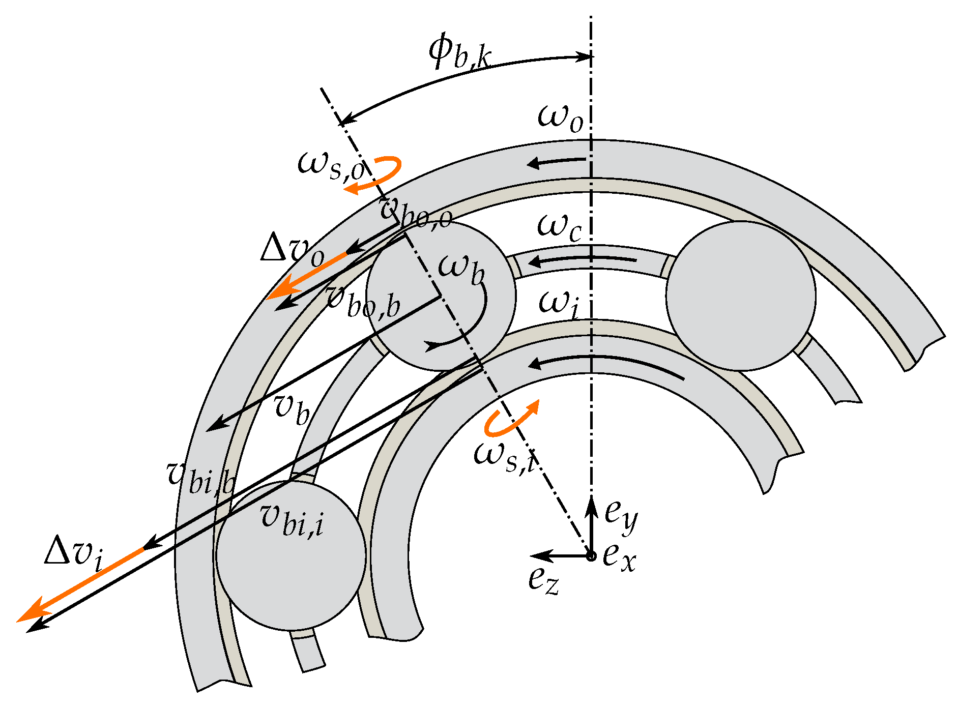
Figure 5.
Power loss, velocity and pressure in the contact ellipse.
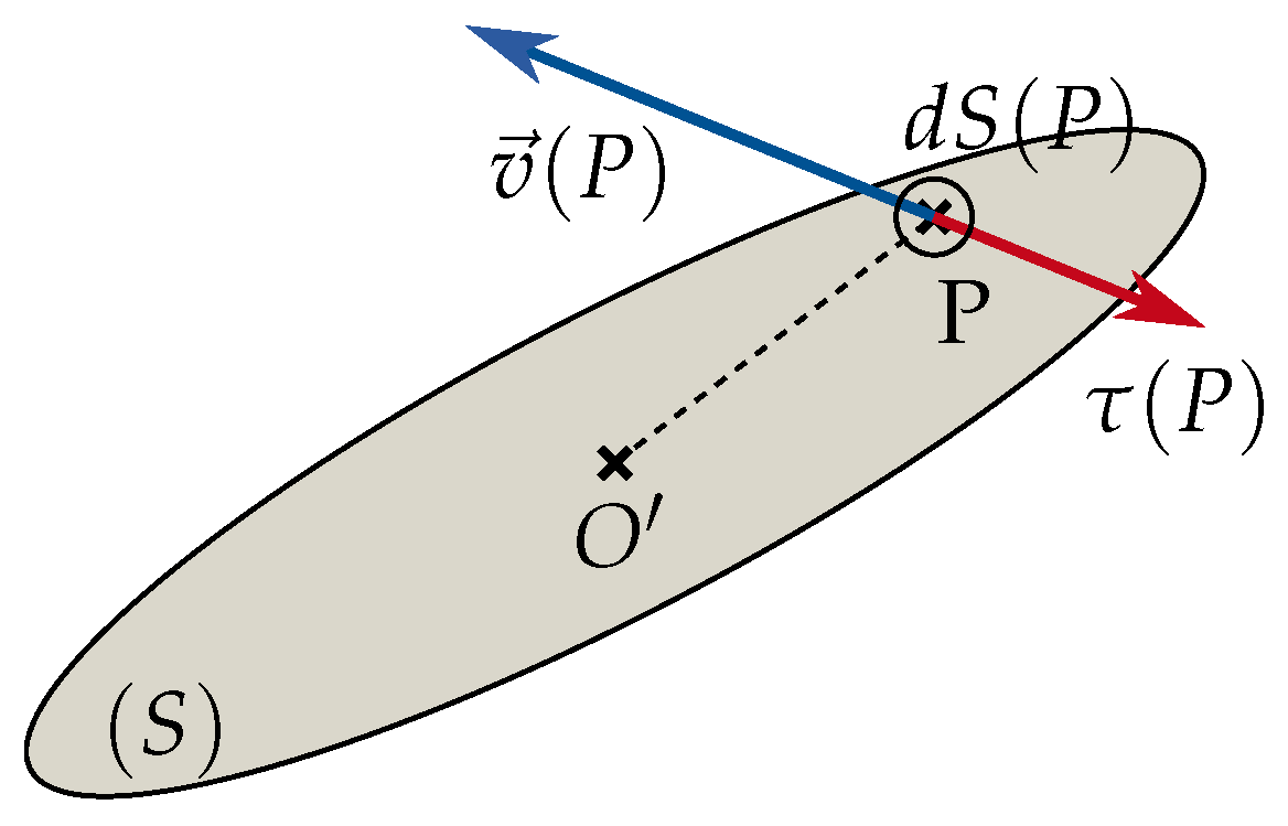
Figure 6.
Finite element model of an elastic bearing outer ring.

Figure 7.
Visualized bearing displacements with elastic outer ring.

Figure 8.
Inner ring displacement according to radial force at different rotational speeds.
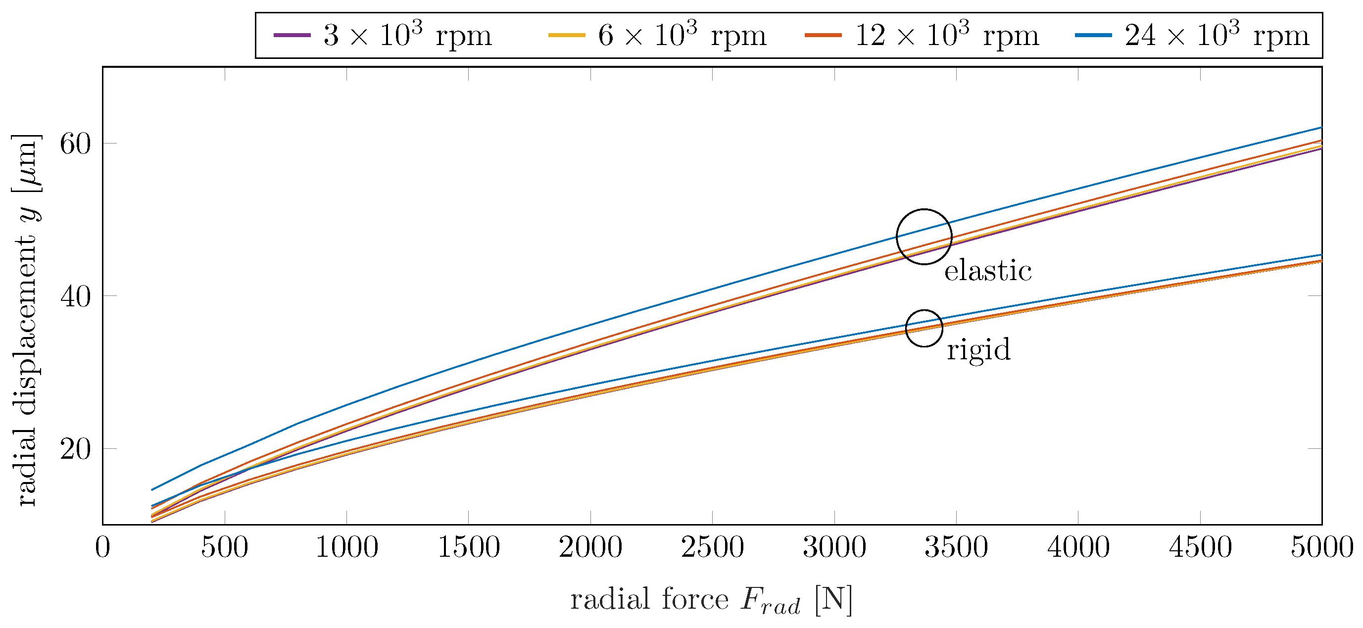
Figure 9.
Radial bearing stiffness according to radial force at different rotational speeds.
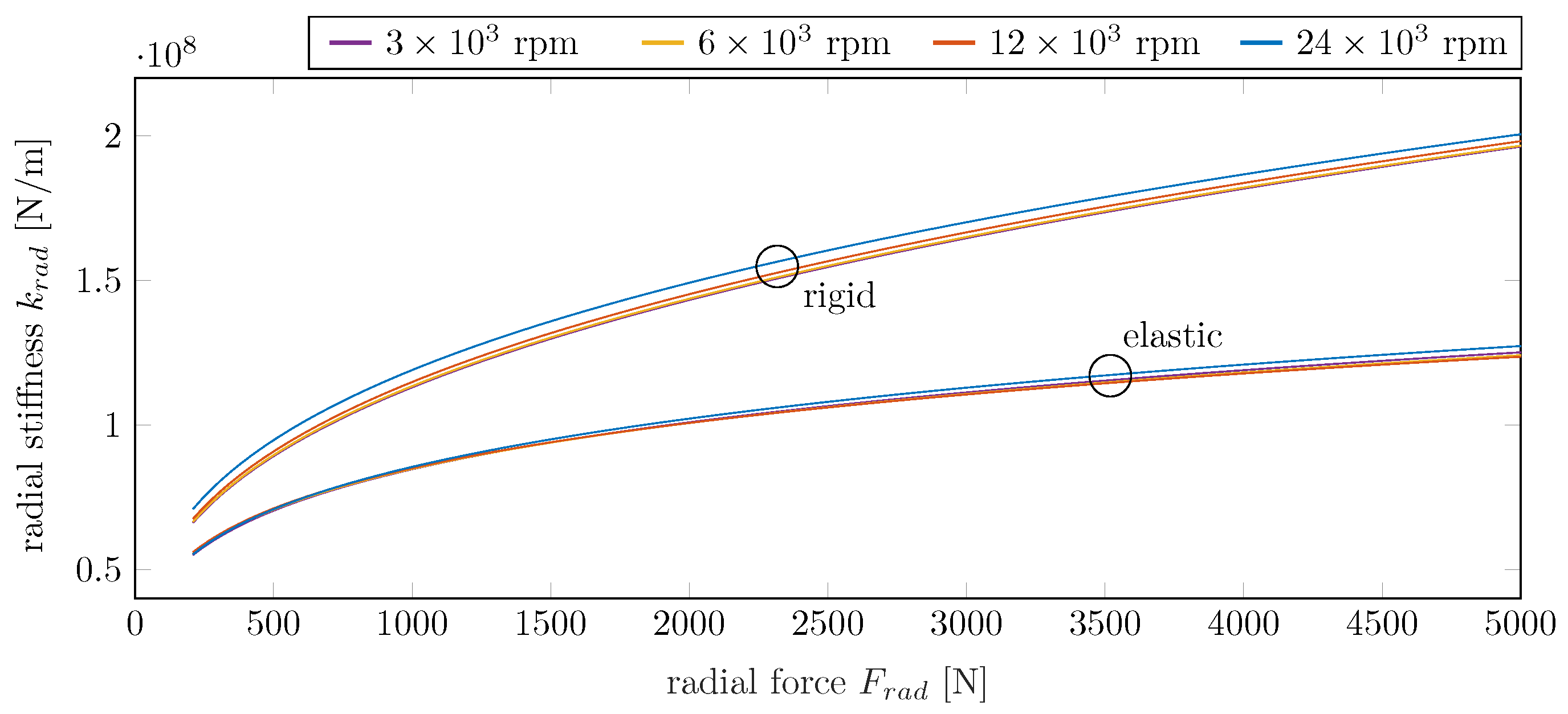
Figure 10.
Inner ring orbit over time at constant radial load and rotational speed.

Figure 11.
Inner ring displacement over time at constant radial load and rotational speed.

© 2017 by the authors. Licensee MDPI, Basel, Switzerland. This article is an open access article distributed under the terms and conditions of the Creative Commons Attribution (CC BY) license (http://creativecommons.org/licenses/by/4.0/).
Share and Cite
MDPI and ACS Style
Wagner, C.; Krinner, A.; Thümmel, T.; Rixen, D. Full Dynamic Ball Bearing Model with Elastic Outer Ring for High Speed Applications. Lubricants 2017, 5, 17. https://doi.org/10.3390/lubricants5020017
AMA Style
Wagner C, Krinner A, Thümmel T, Rixen D. Full Dynamic Ball Bearing Model with Elastic Outer Ring for High Speed Applications. Lubricants. 2017; 5(2):17. https://doi.org/10.3390/lubricants5020017
Chicago/Turabian StyleWagner, Christian, Andreas Krinner, Thomas Thümmel, and Daniel Rixen. 2017. "Full Dynamic Ball Bearing Model with Elastic Outer Ring for High Speed Applications" Lubricants 5, no. 2: 17. https://doi.org/10.3390/lubricants5020017
Note that from the first issue of 2016, this journal uses article numbers instead of page numbers. See further details here.