A Study of Lubricant Inertia Effects for Squeeze Film Dampers Incorporated into High-Speed Turbomachinery


Department of Mechanical and Industrial Engineering, University of Toronto, Toronto, ON M5S 3G8, Canada
*
Author to whom correspondence should be addressed.
Lubricants 2017, 5(4), 43; https://doi.org/10.3390/lubricants5040043
Submission received: 12 September 2017
/
Revised: 24 October 2017
/
Accepted: 29 October 2017
/
Published: 31 October 2017
(This article belongs to the Special Issue Bearings in Turbomachinery)
Abstract
:This work proposes a numerical model that incorporates the effect of lubricant inertia on the hydrodynamic pressure distribution, fluid film reaction forces, and the fluid velocity component profiles for finite-length open-ended squeeze film dampers (SFDs). Firstly, the thin film flow equations for the SFD in presence of fluid inertia effects are introduced. Furthermore, a small first-order perturbation by means of the expressions for the fluid film velocity components and the lubricant pressure distribution that are expanded in power series of the squeeze film Reynolds number is applied to the flow equations. Subsequently the developed lubricant flow equations are solved to develop expressions for the velocity component profiles and the hydrodynamic pressure distribution in SFDs. The pressure expression is numerically solved by using Gauss–Seidel method with finite difference discretization. Moreover, the fluid film reaction forces are determined by numerically integrating the hydrodynamic pressure expressions over the journal surface. Additionally, the proposed pressure distribution expression and the numerical SFD forces are incorporated into a simulation model and the simulation results are compared with the existing models in the literature under different operating conditions, including eccentricity ratios and inertia effects (i.e., Reynolds numbers). The simulation results demonstrate the significant influence of both convective and temporal (i.e., unsteady) lubricant inertia terms on the SFD hydrodynamic pressure distribution and the fluid film reaction forces. Furthermore, the proposed SFD model is incorporated into a multi-mass flexible rotordynamic model to evaluate the effect of SFD fluid inertia on the mass unbalance induced steady-state vibrations of the rotor and the nodal transient orbits by implementing finite element method and transient modal integration with predictor–corrector solver. The results of the analysis demonstrate the significant effect of fluid inertia on the resonance frequencies of the rotor and the steady-state vibration amplitudes and the transient orbits at the resonance zone.
1. Introduction
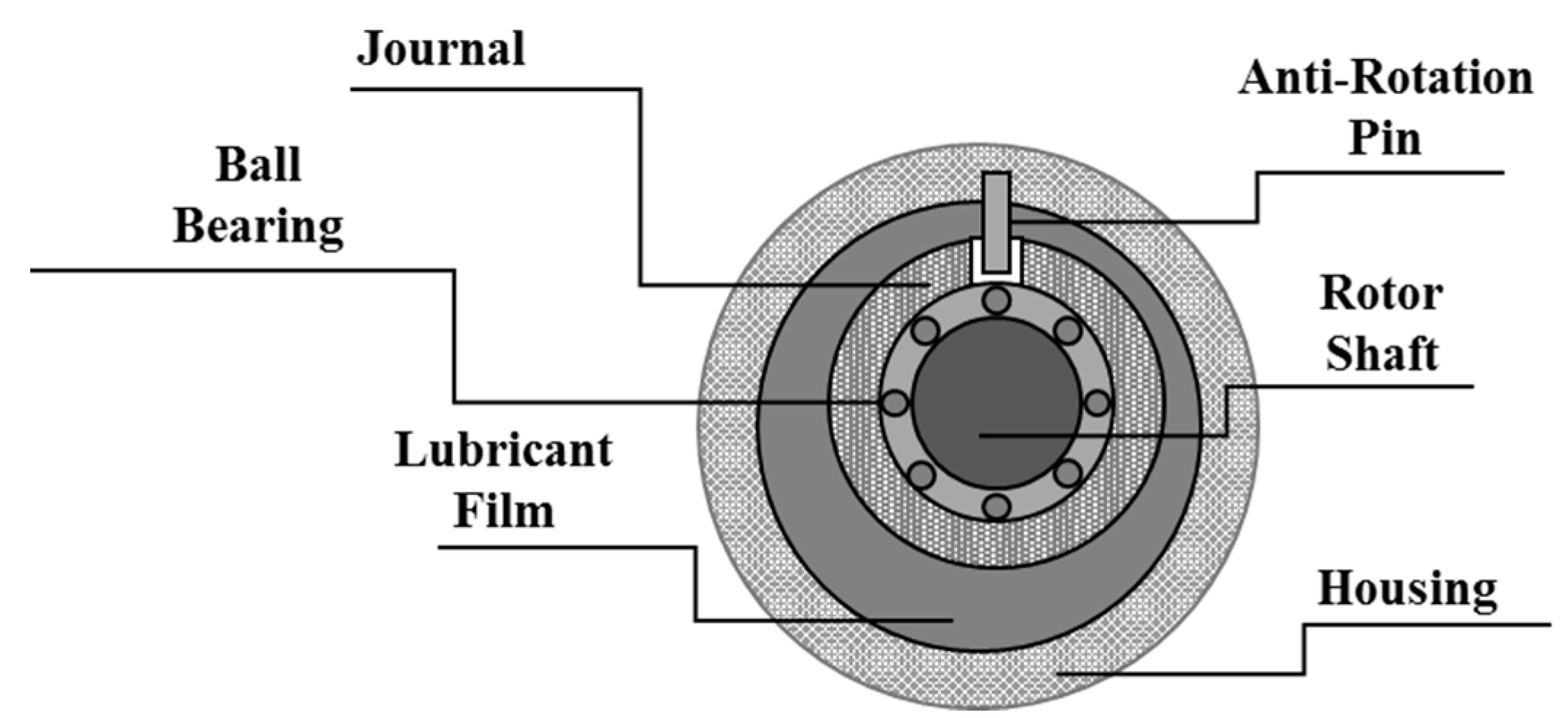
Unbalance induced vibrations are the main source of structural vibrations in high-speed turbomachinery. This mass unbalance is associated with the limitations and imperfections in manufacturing rotor systems and leads to a synchronous load cycle in the rotor. Squeeze film dampers are essential components in high-speed turbomachinery, including aircraft jet engines, high performance compressors, gas turbines, and automotive turbochargers, that are incorporated to attenuate or completely suppress the steady-state unbalance induced vibration amplitudes at the resonance frequencies, reduce the forces transmitted to the supports, and to ensure the stable operation of the system. Figure 1 demonstrates the geometry of a conventional SFD. A typical SFD consists of a stationary outer bearing (i.e., the bush) and an inner journal with approximately identical diameters. The journal is assembled on the outer surface of a rolling element and is prevented from rotation by using an anti-rotation mechanism. The annular region between the journal and the housing is filled with a lubricant. The precession motion of the journal is induced by residual unbalance of the rotor and generates a hydrodynamic squeeze film pressure distribution that applies reaction forces over the journal, providing the damping force to attenuate the transmitted forces and in turn reducing the rotor vibration. The dynamic force response of SFDs is determined by the damper geometry, operating speed, and lubricant properties. Furthermore, SFDs do not produce direct stiffness; a suitable degree of stiffness is introduced by using retaining springs parallel to the squeeze film or by using a pair of elastomer O-rings in radial disposition.
The pioneering work by Cooper [1] demonstrated the benefits associated with the rotor operation from coupling of a damping element, represented by an oil squeeze film, to an elastic element placed within the rotor support. Ever since, research works have focused on providing greater insight into different features of SFDs, including the effect of lubricant inertia. According to classic lubrication theory, the pressure distribution in the thin film region of a hydrodynamic journal bearing is determined by using the Reynolds equation, where it is assumed that the inertial forces are negligible relative to the viscous forces (i.e., ) [2]. In modern turbomachinery, increasing velocity and size of rotors as well as application of low-viscosity lubricants requires the fluid inertia effect to be included in the design and analysis of journal bearings. The effect of fluid inertia for thin films and hydrodynamic journal bearings has been considerably studied in the literature. Smith [3] used simplified journal bearing geometries, including the short and long bearing models, to determine the effect of fluid inertia on the dynamic characteristics of journal bearings. He concluded that the effect of fluid inertia introduces an added mass to the rotor system, which significantly influences the dynamic characteristics of short stiff rotors. Typically, the proposed fluid inertia models assume circular-centered orbits (CCOs) of the journal center. Circular-centered orbits of the journal center is a very common type of journal motion in industrial applications of squeeze film dampers, including vertical rotors mounted on SFDs, horizontal rotors mounted on SFDs with centralizing springs, rotors operating close to critical velocities, and for rotor response to large unbalance forces [4]. Additionally, several investigations [5] have assumed small amplitude motions of the journal center in their corresponding investigations. According to order of magnitude calculations, for small amplitude motions of the journal center, convective inertia terms in the flow equations are negligible relative to unsteady (temporal) inertia terms [6]. However, for large amplitude motions of the journal center, including the displacement at critical speeds, the effect of convective inertia is no longer negligible and should be necessarily incorporated into the calculations.
The force coefficients are the most common representation for the SFD forces in the presence of fluid inertia. In this technique, firstly, the thin film equations are integrated into an expression for the lubricant pressure distribution by adopting either one of the momentum approximation method (aka method of averaged inertia) [7,8,9], the perturbation method [10], or the energy approximation method. Han and Rogers [11,12] have provided a detailed comparison of three approximation methods, namely momentum approximation method, iterative method, and energy method, on the force coefficients for short, long, and finite-length cylindrical SFDs. Subsequently, geometric approximations (i.e., short bearing approximation and long bearing approximation) are applied to the pressure expression to provide an approximate closed-form representation of the lubricant pressure distribution. The closed-form pressure expression is integrated over the journal surface to obtain the fluid film reaction forces (i.e., the tangential and radial components). These forces are nonlinear functions of the velocity and the acceleration of the journal center. The Jacobian matrices of the journal forces with respect to the velocities and the accelerations of the journal center are computed to develop equivalent inertia and damping coefficients respectively. According to the momentum approximation method [13,14], firstly, the flow equations are integrated along the film thickness to represent the flow dynamics in terms of the mean flows, averaged inertia, and wall shear stress differences. Subsequently, the terms in the equations are approximated by assuming that the shape of the velocity profiles is not strongly influenced by the inertia forces [15]. San Andres and Vance [16] implemented the momentum approximation technique to determine the force coefficients for finite-length SFDs executing CCOs. They included convective fluid inertia as well as end seal effects in the calculations. Furthermore, they suggested that the proposed model is strictly valid for small Reynolds numbers (i.e., ). San Andres and Vance [17] analytically investigated the effect of fluid inertia and turbulence on the force coefficients of short and long SFDs. They included both temporal and convective inertia in their analysis. They suggested that at small eccentricity ratios, where the effect of temporal inertia is dominant, an added mass is produced, which corresponds to the radial direct inertia coefficient, however, at large eccentricity ratios, where the effect of convective inertia is superior, this effect is completely reversed. Dousti et al. [18] developed an extended short bearing Reynolds equation that is applicable to both laminar and turbulent flow regimes. Alternatively, according to the perturbation technique [10,19,20], a small first-order perturbation by means of the expressions for the fluid film velocity components and the lubricant pressure distribution that are typically expanded in power series of the squeeze film Reynolds number is applied to the flow equations. This perturbation technique separates the flow equations into a set of inertialess equations that are characterized by using the classic Reynolds equation, and a set of first-order inertial correction equations. According to [16,17,21] it is suggested that the first-order perturbation is applicable for SFD flow regimes with . Finally, the energy approximation [14,22] firstly develops the expressions for the fluid kinetic energy. Subsequently, the Lagrange’s equations along with the Reynolds transport theorem are applied to the energy expressions to obtain the inertia forces. Similar to the momentum approximation technique, in order to develop the fluid expressions, it is assumed that the shape of the velocity profiles is not strongly influenced by the fluid inertia effects.
The force coefficient approach is particularly valuable for rotordynamic analysis, since it directly provides an accelerated estimation of the fluid film reaction forces. However, in order to model the effect of supplementary dynamic lubricant phenomenon on the damping characteristics of SFDs, including lubricant cavitation and lubricant temperature variation, it is additionally required to develop expressions for the lubricant hydrodynamic pressure distribution and the fluid film velocity components. Furthermore, the force coefficients are typically developed for limiting bearing geometries, which makes their predictions inaccurate for arbitrary bearing geometries.
Alternatively, numerical models [23,24,25,26] provide very accurate predictions for the SFD behavior. The bulk flow model [27,28,29] is an additional numerical technique that is used to study the SFD dynamics. In this technique, bulk flow variables are introduced by calculating the average lubricant velocities across the film thickness and are substituted into the flow equations. Subsequently, the bulk-flow model system of equations, including the continuity equation and the momentum transport equation, is solved for the hydrodynamic pressure and the velocity profiles by using finite volume method. The bulk flow modeling along with the finite volume numerical provide superior accuracy for the prediction of the SFD parameters; however, the process is generally computationally very expensive, especially for integration of the SFD model into rotordynamic systems, where the SFD parameters are calculated over a considerable number of iterations.
Additional analytical techniques have been proposed for calculating the closed-form pressure distribution in SFDs [4,21,26,30,31,32,33], however, either the results are strictly valid for specific SFD geometries and configurations, which makes them inapplicable to arbitrary bearing geometries, or they are extremely complicated for integration into rotordynamic models.
Furthermore, the design and application of SFDs in turbomachinery is expansively represented in [34,35]. Typically, the rotordynamic models incorporating SFDs are categorized as follows: (1) Rigid Rotor Model; (2) Simple Flexible Rotor Model; and (3) Complex Flexible Rotor Model. The rigid rotor model assumes that the flexibility of the rotor shaft is neglected and represents the equation of motion of the rotor based on the relative position, velocity, and acceleration of the center of the SFD bearing, the center of the SFD journal, and the mass center of the rotor. The dynamics of a rigid rotor incorporating SFDs and fluid-film bearings was investigated in several studies [36,37,38,39]. The simple flexible rotor model assumes that the total mass of the rotor is either concentrated in the center or in the middle plane of the rotor, or alternatively it is distributed between the rotor center of mass and the center of the bearings. The steady-state orbit whirls of a simple flexible rotor supported by SFDs was investigated in [40,41,42]. In many practical examples, the number of degrees of freedom (DOFs) represented by the simple flexible rotor model is insufficient to provide an accurate approximation of the system dynamics. In this case, the continuous rotor model is discretized and a finite number of DOFs are introduced. The dynamics of multi-mass and multi-degrees of freedom (MDOF) rotors supported with SFDs is theoretically studied in [43,44]. The precedent studies assumed that the effect of lubricant inertia on the fluid film reaction forces in SFDs is negligible and either used the complete or the approximate (i.e., long bearing and short bearing approximations) Reynolds equation to represent the SFD dynamics. For large propulsion turbines and aero-engines the operating SFD squeeze Reynolds number is moderately large, typically on the order of one to twenty [45] and the effect of fluid inertia can no longer be neglected for those applications.
This work proposes a numerical model that represents the effect of lubricant inertia on the hydrodynamic pressure distribution, fluid film reaction forces, and the fluid velocity component profiles for finite-length open-ended squeeze film dampers (SFDs). The proposed models in this work are powerful tools that provide precise and accelerated evaluation of the SFD hydrodynamic pressure distribution, velocity profiles, and fluid film reaction forces, for application in rotordynamic models as well as the study of the effect of lubricant cavitation and lubricant temperature variation on the damping effectiveness of SFDs. The following sections describe the derivation of the analytical pressure and velocity expressions. Subsequently, the proposed expressions are incorporated into a simulation model and the performance of the SFD models are evaluated under different operating parameters. Finally, the proposed SFD model is incorporated into a flexible multi-mass rotordynamics model, to determine the effect of SFD lubricant inertia on the transient orbits and the steady-state unbalance induced vibrations of rotor systems.
2. Governing Equations
The SFD configuration in this work is a symmetric damper about its mid plane with open ends (i.e., no seal). The geometry of the system is represented in Figure 2. An orthogonal Cartesian coordinate system {x,y,z} is fixed in the plane of the lubricant, where the z-axis is perpendicular to the plane of motion. Furthermore, an orthogonal Cartesian system {x′,y′,z′} translating with angular velocity Ω is introduced, where the x′-axis is perpendicular to the line connecting the centers of the inner and outer cylinders, and the y′-axis is in the direction of the minimum thickness. The angle θ′ starts from the origin of the fixed Cartesian system and the angle θ is measured at the maximum film thickness in the direction of the whirling motion. Finally, a fixed inertial coordinate system {X,Y} is defined at the center of the bearing.
The dynamic behavior of a viscous Newtonian fluid within boundaries is generally characterized by using the 3-dimensional continuity and Navier–Stokes equations as follows [2]:
where Equation (1) is the continuity equation corresponding to the conservation of mass within the fluid boundaries; and Equations (2) correspond to the conservation of momentum within the fluid boundaries. The terms in Equations (1) and (2) are expanded as follows [46]:
Furthermore, it is assumed that [46]:
- The body force terms are small compared to the viscous, inertia, and pressure terms.
- According to an order of magnitude analysis, the velocity gradients and are large compared to all other velocity gradients.
- The lubricant is Newtonian, incompressible (i.e., density gradient is zero), and iso-viscous (i.e., the viscosity gradient is zero).
Applying the above assumptions to Equations (3)–(6) gives:
Additionally, according to the thin film assumption in hydrodynamic lubrication theory, which is characterized by the small ratio of film thickness to the bearing’s other physical dimensions, i.e., , it is concluded that:
- The effect of the curvature of the film is negligible; hence a linear coordinate system is used to describe the lubricant dynamics.
- The variation of the pressure across the film is negligible (i.e., ).
Based on the preceding description, for an incompressible and iso-viscous lubricant, the flow equations in the SFD are reduced to:
Subsequently, in order to demonstrate the dependence of the fluid inertia terms on the Reynolds number, the flow equations are normalized by introducing dimensionless parameters as follows:
The dimensionless parameters in Equation (15) are substituted into Equations (11), (12) and (14) as follows:
Additionally, the dimensionless velocity boundary conditions for the lubricant are defined as follows:
Moreover, the boundary conditions for the hydrodynamic pressure in an open ended SFD are given by:
- The pressure is periodic and continuous in the circumferential direction (θ), i.e.,
- The pressure equals atmospheric pressure at the axial ends of the bearing, i.e.,
- The hydrostatic pressure must be above the liquid cavitation pressure, i.e.,
where Pcav is the saturation pressure of the lubricant or the saturation pressure for release of entrapped gases, typically ambient pressure.
Subsequently, a small first-order perturbation by means of the expressions for the fluid film velocity components and the lubricant pressure distribution that are expanded in power series of the squeeze film Reynolds number is introduced as follows:
The above approximation separates the pressure and the velocity components into a zeroth-order inertialess term and a first-order inertial correction component. Substituting Equations (20)–(23) into Equations (16)–(18) and assuming that the inertial expressions in the equations are approximated by using zeroth-order velocities [10] gives:
According to the expressions for the inertialess continuity and momentum transport equations, the left-hand side of Equations (24)–(26) is equal to zero. Consequently, the following set of zeroth-order inertialess equations and first-order inertial equations are introduced:
2.1. Zeroth-Order Equations
2.2. First-Order Equations
The zeroth-order velocity components and pressure distribution are determined by integrating Equations (27)–(29) in the radial direction and applying the velocity and pressure boundary conditions as follows [24]:
where Equation (38) is referred to as Reynolds equation [2], which is adopted to determine the inertialess lubricant pressure field. Furthermore, according to Equation (38):
Substituting Equation (39) into Equation (37) gives:
Subsequently, the inertialess velocity components in Equations (35), (36) and (40) are substituted into Equations (32) and (33) to determine the first-order velocity profiles. Firstly, according to Equation (32):
Equation (41) is integrated twice in the radial direction and is solved for the first-order circumferential velocity component. Furthermore, the integration constants are determined by applying the velocity boundary conditions in Equation (34), hence:
Similarly, the axial first-order velocity component is calculated as follows:
Subsequently, in order to eliminate the radial velocity component, Equation (31) is integrated along the film thickness and the velocity boundary conditions are applied:
where, the first-order lubricant flows are defined as [2]:
Substituting Equation (44) into Equation (45) gives:
Integrating the first-order velocity expressions in Equations (42) and (43) along the film thickness and substituting into Equation (46) gives:
Equation (47) provides a Reynolds-like expression that characterizes the first-order pressure distribution. The total fluid film pressure distribution is calculated by using Equation (23). Additionally, the total fluid film pressure distribution is numerically integrated over the journal surface to calculate the fluid film reaction forces as follows:
where θ1 to θ2 is the positive range of the pressure distribution. The following section describes a numerical scheme that determines the zeroth-order and first-order pressure distributions.
3. Numerical Solution
This section describes the procedure to determine the pressure distribution and the fluid film forces in SFDs by numerically solving Equations (38) and (47). In order to determine the numerical solution, firstly, a solution domain is defined for the problem. Subsequently, the partial differential pressure expressions are discretized over the solution domain by using finite difference approximation. Finally, an iterative Gauss–Seidel numerical algorithm with successive over-relaxation (SOR) is developed to calculate the point-wise pressure distribution in the thin film domain.
3.1. Zeroth-Order Pressure Solution
In order to calculate the total fluid film pressure distribution, the zeroth-order pressure distribution must be first determined. The zeroth-order pressure distribution is characterized by Equation (38). This equation is expanded and discretized by applying finite difference approximation. The detailed description of the numerical procedure is provided in Appendix A. The discretized zeroth-order pressure expression is produced as follows:
where
In general, Reynolds equation is classified as an elliptical PDE. Assuming that the lubricant is incompressible and iso-viscous, and the journal center executes CCO whirls, the following Gauss–Seidel numerical procedure is used to determine the fluid film pressure distribution for a specified SFD eccentricity ratio:
- The boundary points are initialized to their prescribed values, and the interior points are adjusted to zero.
- Equation (49) is iteratively solved for the interior points.
- The iteration is only interrupted when the solution error reaches a convergence criterion.
- Finally, a SOR technique is used to accelerate the convergence of the solution:where k denotes the iteration number.
3.2. First-Order Pressure Solution
The numerical procedure that is employed to determine the first-order pressure distribution is very similar to the one that was described for the zeroth-order pressure. The first-order pressure distribution in the fluid film is characterized by Equation (47). Similarly, this equation is expanded and discretized by applying finite difference approximation. The detailed representation of the numerical procedure is provided in Appendix B. The discretized first-order pressure expression is produced as follows:
where
Subsequently, Equation (52) is iteratively solved by using the numerical procedure that was described in the previous section. Finally, the total pressure distribution is determined based on Equation (23) and the fluid film reaction forces are computed by numerically integrating the total pressure field over the journal surface:
4. Results and Discussion
This section represents the simulation results for the pressure distribution and the fluid film reaction forces for the proposed hydrodynamic SFD model. The simulation results are provided at different operating conditions, including eccentricity ratios and Reynolds numbers (i.e., inertia effects). The numerical algorithm that was developed in the previous section is incorporated into Matlab and Simulink® to evaluate the effect of SFD operating parameters on the lubricant pressure distribution and the fluid film reaction forces in SFDs. In order to investigate the contribution of convective inertia on the SFD dynamics, the results of the simulations are compared against [24], where the effect fluid inertia is described for SFDs executing small-amplitude CCOs. According to an order of magnitude analysis, for small amplitude motions of the journal center, convective inertia terms in the flow equations are negligible relative to unsteady (temporal) inertia terms [6]. However, for large amplitude motions of the journal center, including the displacement at critical speeds, the effect of convective inertia is no longer negligible and should be necessarily incorporated into the calculations. Additionally, this work incorporates a π-film cavitation model to determine the fluid film reaction forces in the SFDs, however, in order to compare the pressure profiles at different SFD operating conditions, the negative intervals of the pressure calculations are included in the figures.
Furthermore, the fluid film reaction force components for the complete inertia model (i.e., both convective inertia and temporal inertia) and the temporal inertia model in [24] are compared with the force coefficient model developed by Vance [47]. Vance has developed the force coefficients for short-length open-ended SFDs by using the π-film assumption (i.e., film cavitation region is developed in half the damper circumference). The force coefficients are represented as follows:
The fluid film reaction force components are calculated based on the force coefficients in Equations (56)–(59) as follows:
where
and
where
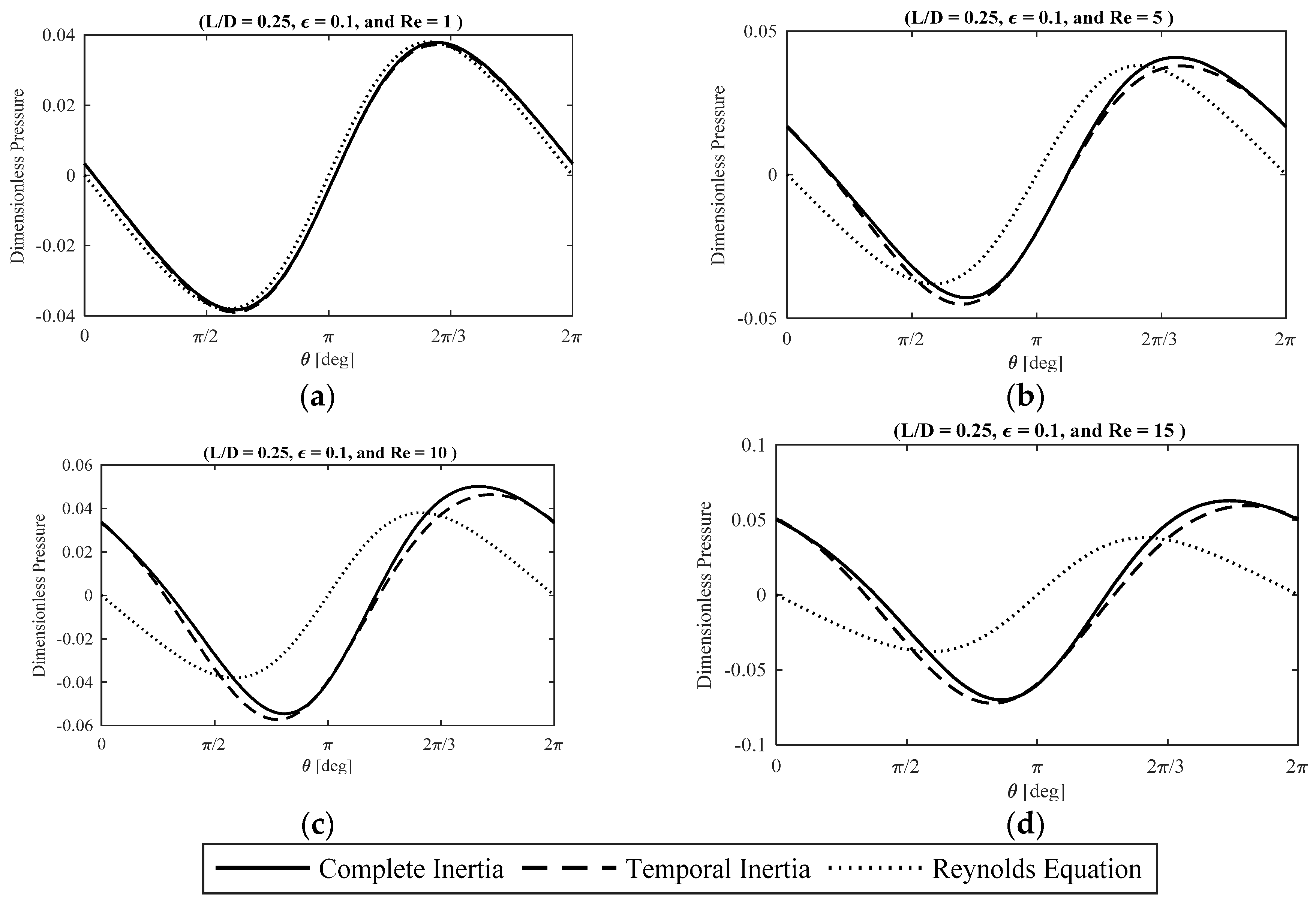
Figure 3 represents the effect of fluid inertia on the dimensionless lubricant pressure distribution at the bearing midplane () at small eccentricity ratios for Reynolds equation (i.e., no inertia effect), the temporal inertia model in [24], and the proposed complete inertia model. In general, the fluid inertia effect causes a significant elevation in the pressure magnitude, a change in the shape of the pressure profile, and a phase shift of the pressure peak in the direction of the journal precision. At small Reynolds numbers, the influence of the viscous forces makes the pressure profile closer to a sinusoid, however, at moderate and large Reynolds numbers the pressure is in phase with the gap acceleration and transforms into a cosine wave shape. Furthermore, the temporal inertia model and the complete inertia model shows demonstrate a close agreement at small eccentricity ratios for a small to moderately large range of inertia effects.
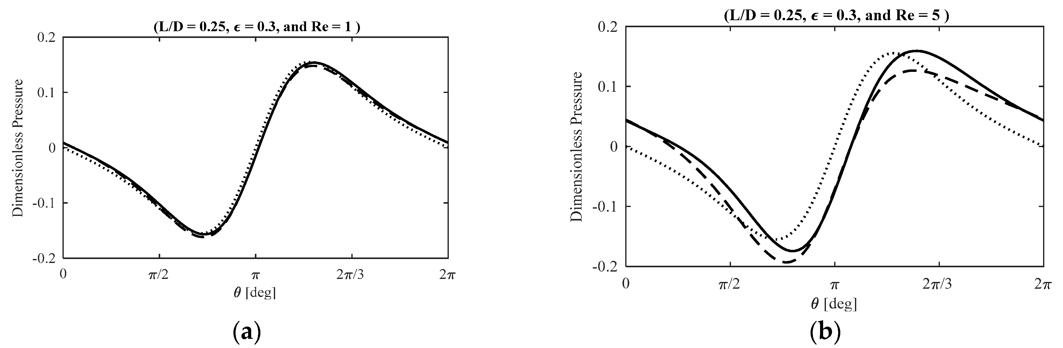
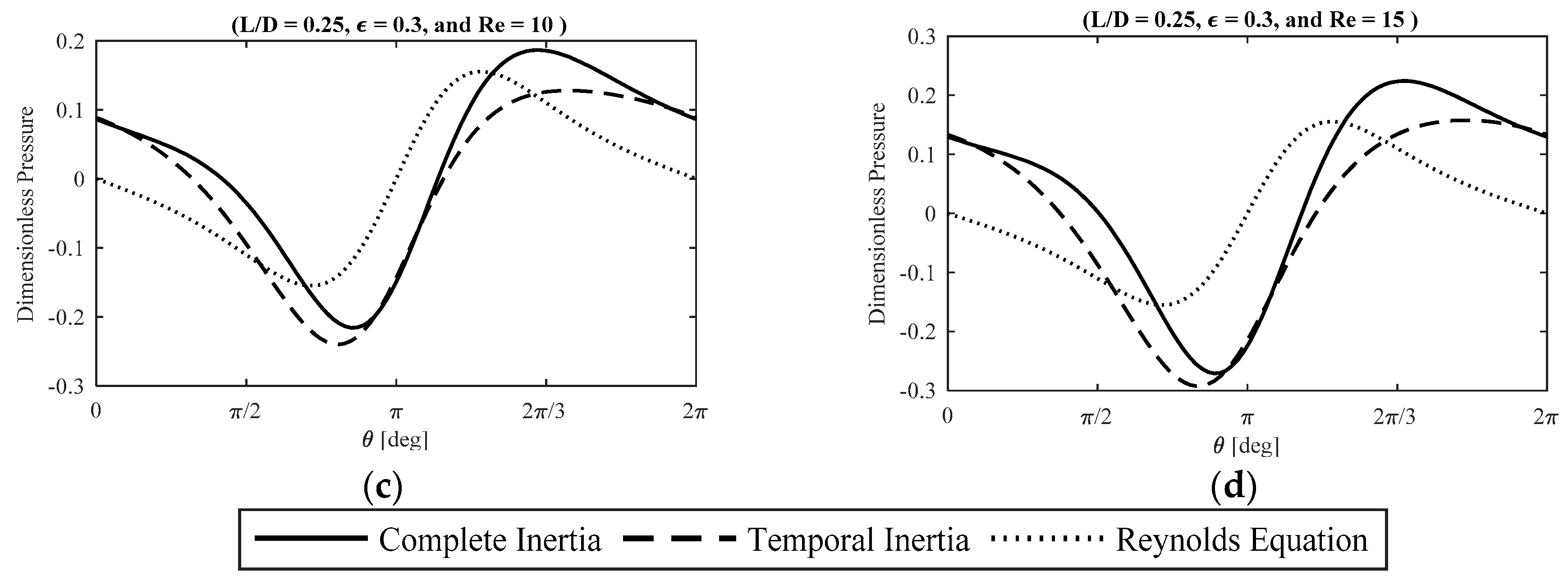
Figure 4 illustrates the effect of fluid inertia on the dimensionless lubricant pressure distribution at the bearing midplane () at moderate eccentricity ratios. At small Reynolds numbers, the temporal inertia model and the complete inertia model demonstrate a very close agreement. However, by increasing the effect of fluid inertia (i.e., Reynolds number), the discrepancy between the results of the two models grows noticeably. At moderately small and moderate Reynolds numbers, the divergence between the results of the two models is more significant in terms of the pressure magnitude, while the shape and the phase of the profile is unaffected. However, at moderately large Reynolds numbers, the effect of convective inertia terms considerably influences the shape of the pressure profile.
Figure 5 demonstrates the effect of fluid inertia on the dimensionless lubricant pressure distribution at the bearing midplane () at large eccentricity ratios. For large eccentricity ratios of the journal center, the effect of convective inertia effects is very significant on the pressure magnitude even at moderately small Reynolds numbers. Further increasing the effect of fluid inertia results in the noticeable divergence of the two pressure profiles. The results imply that the effect of convective fluid inertia is very significant at large eccentricity ratios, including at the resonance frequencies of the rotor systems incorporating SFDs.
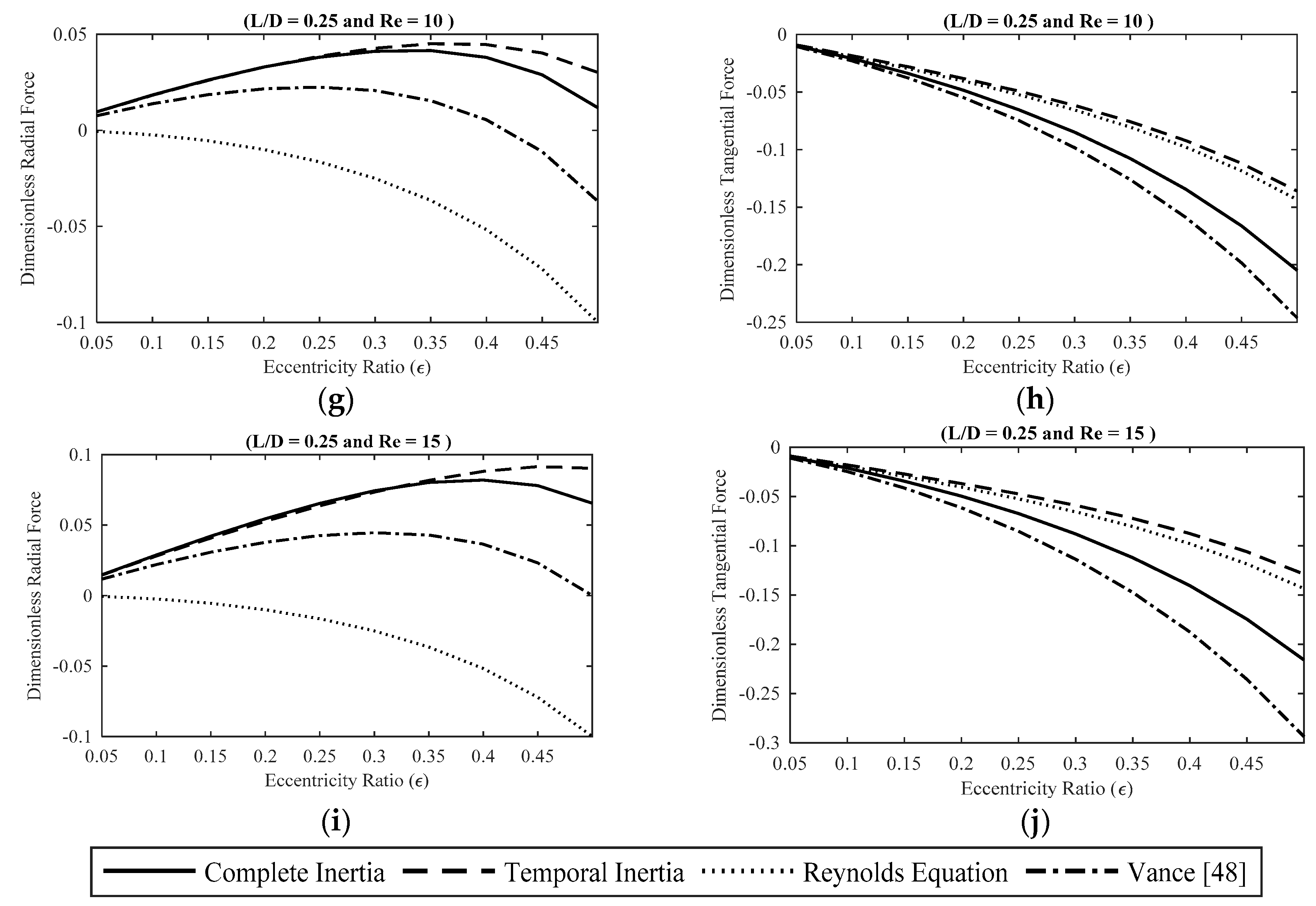
Figure 6 represents the effect of fluid inertia on the SFD fluid film reaction forces at small eccentricity ratios for four SFD models, namely no inertia effects, temporal inertia effects, complete inertia effects, and the force coefficient model [47]. The fluid forces are calculated by numerically integrating the lubricant hydrodynamic pressure distribution over the journal surface. For a π-film SFD model at small to moderate inertia effects, the contribution of the inertia forces to the radial force component is a positive value. This positive contribution is added to the negative viscous radial forces and reduces the magnitude of the radial force component relative to the inertialess model, which diminishes the likelihood of bi-stable rotor operation [16]. Furthermore, the magnitude of the inertialess radial forces is negative, meaning that the force is directed towards the center of the bearing (i.e., inwards). However, introducing the effect of fluid inertia initially changes the value of the forces to positive at small eccentricities, demonstrating the outward direction of the forces (i.e., outwards). Subsequently, at larger eccentricity ratios, the value of the radial forces switches back to negative, meaning that the force direction is once again towards the center of the bearing. Moreover, the contribution of the inertial forces to the tangential fluid film reaction forces is a negative value, and is added to the already negative purely viscous tangential forces, thus increasing the total magnitude of the tangential forces. Furthermore, the comparison between the temporal inertia model and the complete inertia model shows that at small Reynolds numbers the results of the two models are in a close agreement. At moderately small inertia effects, the discrepancy between the results of the two models is noticeable. At small eccentricity ratios, the radial forces suggested by the two models are in close agreement, however, increasing the eccentricity ratio leads to the divergence of the force calculations. The discrepancy between the force calculations is much more significant for the tangential force components, demonstrating the substantial influence of convective inertia effects on the SFD tangential forces. Further increasing the Reynolds numbers results in a more significant discrepancy between the radial force calculations at large eccentricity ratios and the tangential forces.
Additionally, the results of the complete inertia model and the force coefficient model are in close agreement for small to moderate Reynolds numbers. Increasing the Reynolds number leads to the divergence of the force calculations, since it is suggested that the force coefficient model is mostly accurate at small to moderate inertia effects. Furthermore, the force coefficient model is derived by incorporating the short bearing approximation, which reduces the accuracy of the calculations at moderate and large eccentricity ratios.
Subsequently, the proposed SFD model is incorporated into a multi-mass flexible rotor model to study the effect of SFD inertia forces on the steady-state mass unbalance induced vibrations and the transient orbits of the rotor system. The details of the proposed rotordynamics model is given in [48]. The rotor model is discretized by using finite element analysis (FEA) into Timoshenko beam elements [49] and the element mass matrix, stiffness matrix, and gyroscopic effects matrix are defined and assembled to provide a global rotor system model. Furthermore, the proposed nonlinear cavitated SFD model with centering springs, including lubricant inertia effects, is incorporated into the rotordynamic model. Finally, a predictor–corrector transient modal integration technique is implemented to determine the transient and the steady-state unbalance response of the rotor system at different operating conditions.
The main components of a conventional rotor system include the shaft, the disk, the mass unbalance, the rolling elements, the SFDs, and the retaining springs. This work applies finite element analysis [50] to determine the vibration amplitudes in the rotor system. In order to apply FEA to the rotor system, firstly, the structure is discretized into subdivisions of simple geometry that are referred to by elements. Subsequently, the elastic, inertia, damping, and external forces and moments on each element (local forces) are expressed in terms of the local coordinates (i.e., translations and rotations). Furthermore, the forces and the moments from every element are assembled together to produce the global forces in terms of the generalized coordinates. Finally, the discretized equation of motion is solved by using numerical techniques. In a rotor system, the shaft is discretized into several beam elements with nodes at both ends of each element. The disks and the bearings are assumed to be attached to the shaft at these nodes. In this work, the rotor vibrations in the lateral and transverse directions are considered. Consequently, each node has four generalized coordinates, including transverse displacements in the x and y directions as well as rotations about x-axis and y-axis. The properties of a rigid disk are determined by using Lagrange’s energy method. It is assumed that the disk strain energy is negligible with respect to the disk kinetic energy. Subsequently, the kinetic energy of the disk due to translation and rotation are calculated, and Lagrange’s energy method is applied to the energy equation to determine the element mass matrix and element gyroscopic matrix for the disk. The shaft contributes mass, stiffness, and gyroscopic effect to the rotor model. Similarly, the stiffness, inertia, and gyroscopic element matrices for the shaft are determined by using Lagrange’s energy method. The element matrices are derived for either the Bernoulli beam model or the Timoshenko beam model (includes both rotary inertia and shear effects). In order to determine the element matrices, firstly, the displacement along the shaft element is approximated by using shape functions. Subsequently, expressions for the kinetic energy and the strain energy are used to determine the element matrices. The strain energy of the shaft is calculated to approximate the element stiffness matrix. The kinetic energy due to the translation of the shaft gives the inertia element matrix and the kinetic energy due to the rotational motion of the shaft gives the gyroscopic effect matrix. The bearing element includes the stiffness and the damping contribution from the rolling elements as well as the stiffness contribution from the retaining springs in the SFDs. The bearings are flexible and absorb energy. It is assumed that the rotor is symmetric, and a disk is located at the axial center of the rotor. Furthermore, the rotor is supported with SFDs at either axial end. The SFDs are assembled on the outer race of two identical rolling elements that the rotor is assembled on. Moreover, the unbalance forces are present only on the centered disk. The equation of motion (EOM) of the rotor system is determined either by using the Lagrange’s energy method. For a conventional rotor system, the EOM is constructed as follows:
where q is a vector that contains the translations and the rotations at the nodes. The element matrices are 8-by-8 for stiffness, gyroscopic effect, and inertia. The effect of bearings, SFDs, and disks are directly incorporated into the corresponding nodes. Furthermore, the global mass, stiffness, and gyroscopic effect matrices are constructed by transforming the local element matrices into global coordinates and assembling the matrices together.
The transient response of the rotor system is determined to evaluate the effect of time variant nonlinear components (i.e., SFDs) on the performance of the rotor system. The most common and inclusive method for computing transient forced vibrations in rotor systems is the transient numerical integration approach. In the transient integration technique, the rotor system degrees of freedom are marched forward in time through a force balance at every time step. This technique allows any nonlinear elements (i.e., SFD forces) to be included directly as long as the forces can be represented as a function of position and velocity. Furthermore, transient modal integration is a powerful technique to determine the transient solution for dynamic systems with large number of degrees of freedom [51,52]. This technique is appealing since it facilitates the elimination of higher frequency modes with little impact on the system dynamics, which yields to significantly lower number of degrees of freedom compared to the direct integration method. Transformation of the rotor equation of motion into modal coordinates gives:
where the model transformation is given by:
and the modal mass and the modal stiffness matrices are given as follows:
and F(t) is the sum of the external forces, including the unbalance forces and the SFD fluid film reaction forces. Assuming that the unbalance mass is attached to the disk, the unbalance force in the rotor is determined as:
where Ω2F0 is the vector of forces and moments acting at the ith node due to a disk with an unbalance, where F0 is given as follows:
Assuming that no other unbalance forces are applied to the rotor system, the rest of the force vector entities are zero. Furthermore, the fluid film reaction forces are calculated by Equation (55). Subsequently, a transformation is applied to calculate the SFD forces in the fixed inertial coordinate (i.e., {X,Y}) as follows:
and
Additionally, a numerical procedure integrating a predictor–corrector technique is incorporated into the simulation model to determine the rotor vibration amplitudes at different frequencies. In this study, the predictor uses backward finite difference method and the corrector uses Newmark–Beta method. The proposed transient modal integration algorithm is represented in Figure 7.
In the simulations, it is assumed that the unbalance forces are present only on the centered disk. Additionally, the rotor shaft is discretized into 20 elements. Table 1 summarizes the rotor and SFD parameters. A schematic diagram of the rotor in the simulations is demonstrated in Figure 8.
Figure 9 represents the effect of SFD viscous forces (i.e., neglecting inertia effect) on the steady-state vibration amplitudes of the rotor system at the disk node for the SFD radial clearance of 1.27 × 10⁻⁴, at the lubricant temperature of 100 °C, and for the three different unbalance magnitudes in Table 1. Firstly, the steady-state vibration amplitudes increase with the unbalance magnitude. Furthermore, even for the case where the effect of fluid inertia is neglected, the steady-state vibrations of the disk center is significantly attenuated at the first resonance frequency (i.e., the first bending mode) by incorporating the SFDs into the rotor system.
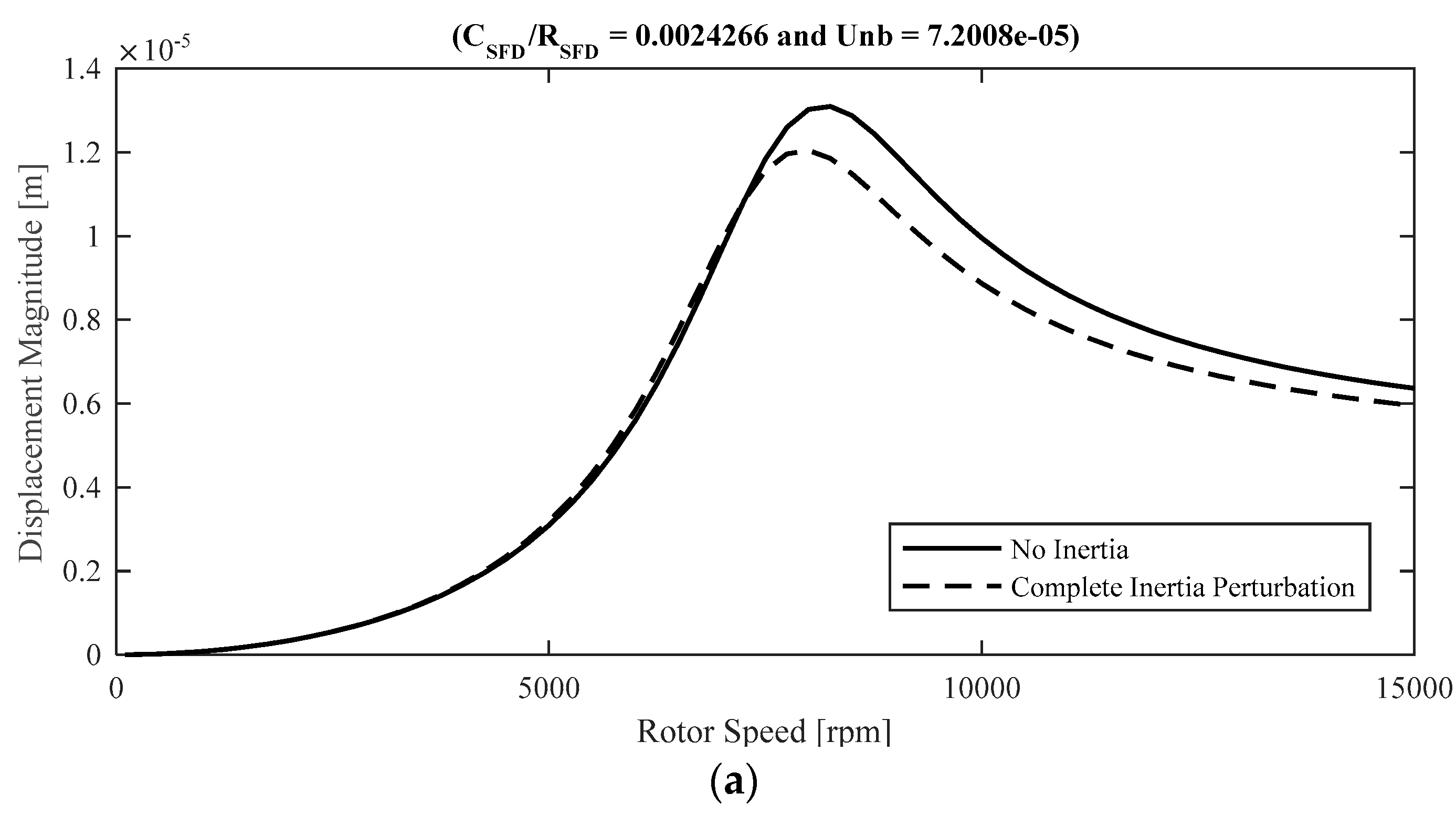
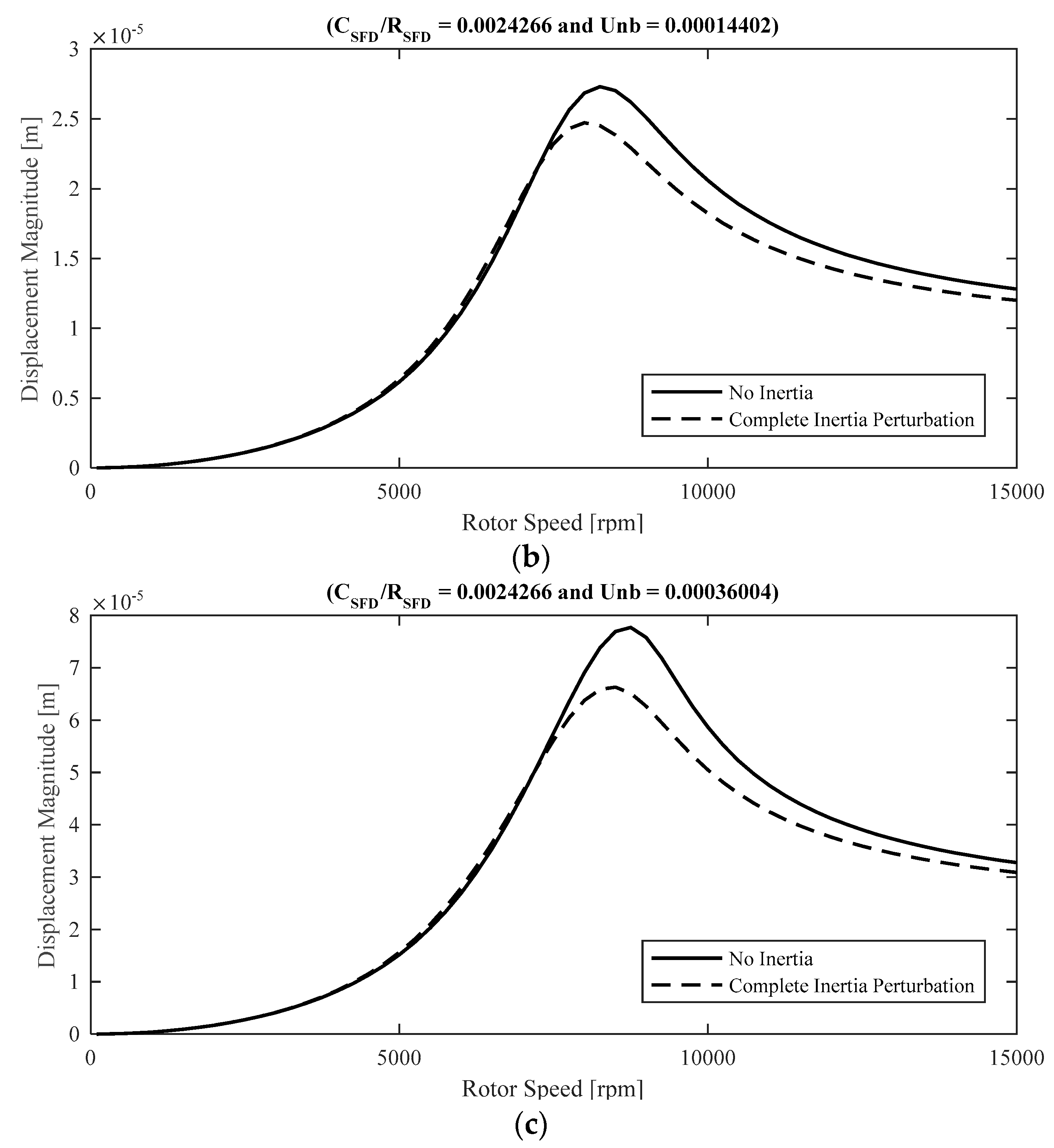
Figure 10 represents the effect of fluid inertia on the steady-state vibration amplitudes of the rotor system at the disk node for two different cases, namely: (1) Viscous SFD model (i.e., no inertia effects) and (2) complete fluid inertia effects. The results are represented at lubricant temperature of 100 °C and for the 3 unbalance magnitudes in Table 1. In general, the fluid inertia effects considerably attenuate the steady-state vibrations at the resonance zone and at large rotor velocities. At small to moderate rotor speeds, the squeeze Reynolds number is relatively small, and the effect of fluid inertia is negligible, consequently, the steady-state vibrations for the two cases is very similar. At the first resonance zone (i.e., first bending mode), the squeeze Reynolds number is moderately large, and the effect of fluid inertia is significant. Additionally, the vibration amplitudes at the resonance frequency zone are noticeably larger, resulting in larger SFD eccentricity ratios. Consequently, at the first resonance zone, the inertial correction component is large and the discrepancy between the results of the two models is noticeable, demonstrating the influence of fluid inertias effects on the suppression of the unbalance induced vibration amplitudes. At the post resonance zone, the rotor speeds are large, which results in the elevation of the Reynolds number and the inertia effects, hence, the inertia correction term remains significant and leads to the reduction of the steady-state vibration amplitudes relative to the no inertia model. Finally, the effect of fluid inertia leads to a shift in the first resonance frequency from 8250 rpm to approximately 8000 rpm. In general, the effect of SFD fluid inertia is represented by and added mass, which is supplemented into the overall rotordynamic system mass, which in turn reduces the first resonance frequency of the system.
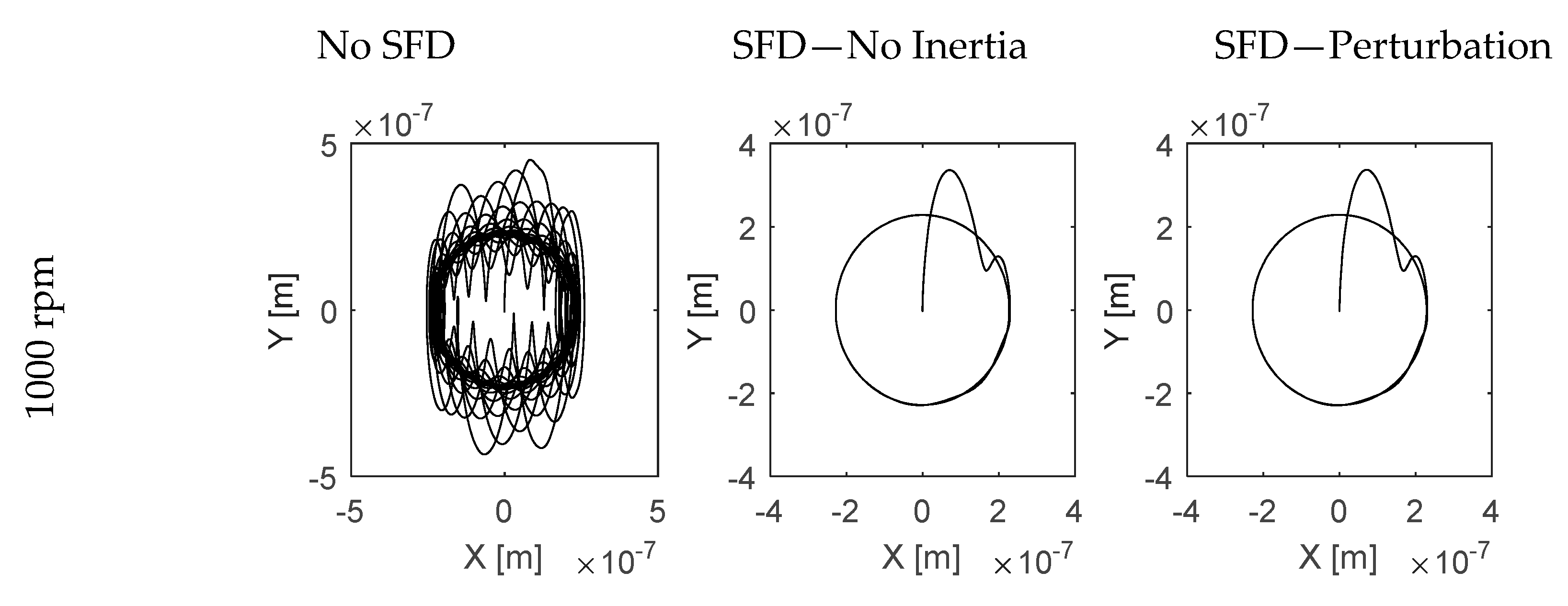
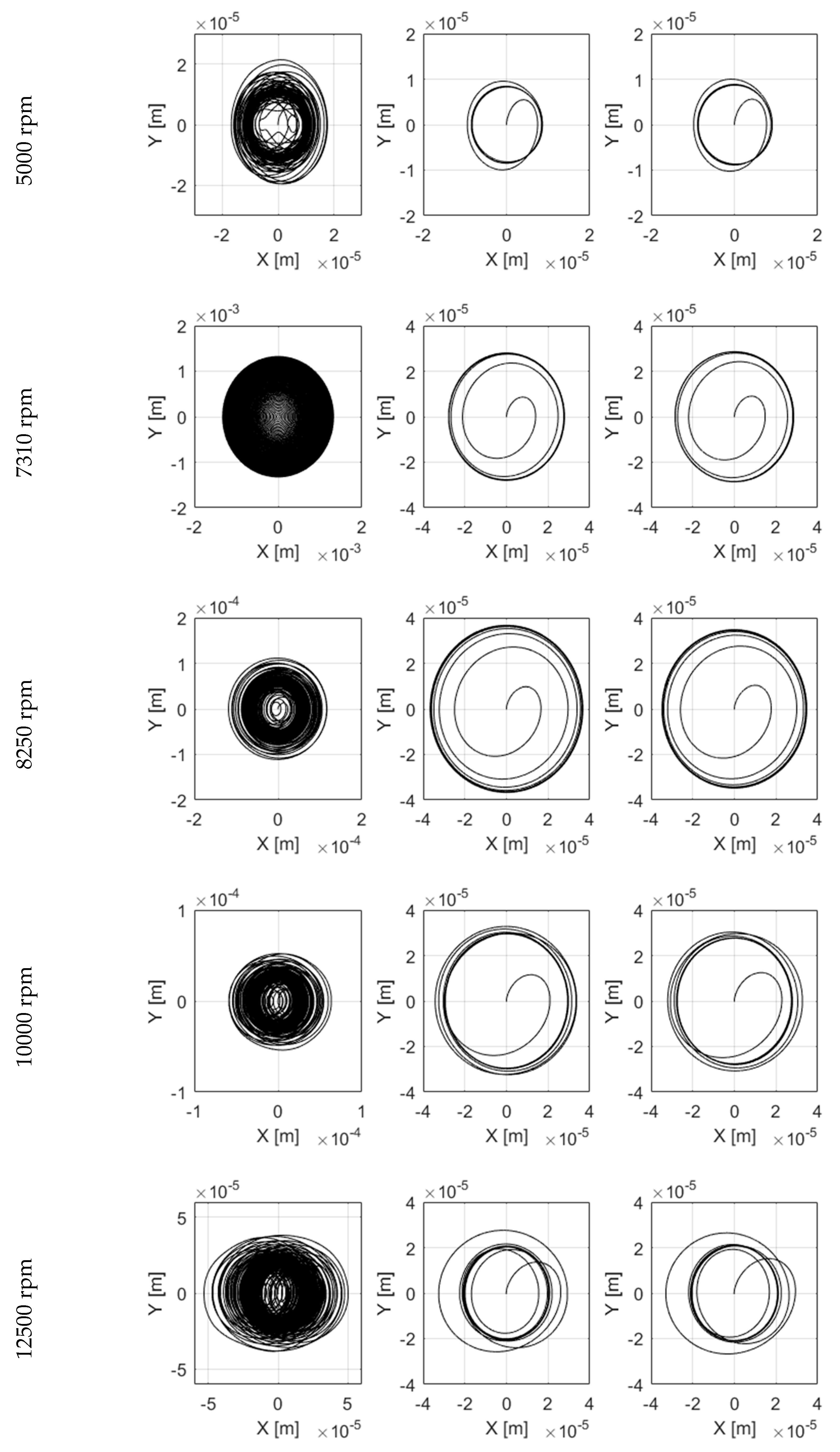
Figure 11 represents the transient orbits of the SFD journal center at the 0.00242 radial clearance ratio and at 0.00036004 kg-m unbalance force at different rotor speeds for three different configurations: (1) No SFD; (2) Viscous SFD model (i.e., no inertia effects); (3) Complete inertia model. At small rotor speeds (1000 rpm and 5000 rpm), the squeeze Reynolds number is relatively small and the results for the three SFD configurations are in close agreement. Furthermore, including the SFD effect significantly accelerates the convergence of the orbits to the steady-state value. At the resonance zone (7310 rpm and 8250 rpm) the squeeze Reynolds number and the orbit radius are relatively larger, and the inertia models demonstrate both significantly faster convergence and smaller orbit radius. At larger rotor speeds (10,000 rpm and 12,500 rpm) the squeeze Reynolds number is moderately large while the orbit radius rapidly declines relative to the resonance zone.
5. Conclusions
This work represented expressions for the hydrodynamic pressure distribution and the lubricant velocity profiles, including fluid inertia effects, for finite-length open-ended squeeze film dampers incorporated into high-speed turbomachinery. The proposed pressure model provides very close agreement compared to the existing pressure models, including limiting geometry models. Moreover, a numerical procedure is proposed to solve the model for point-wise pressure distribution, which is significantly more computationally efficient relative to the bulk-flow technique. Finally, the numerical pressure field is numerically integrated over the journal surface to determine the fluid film reaction forces.
The analysis of the pressure model confirms the significant contribution of the fluid inertia to the dynamics of the lubricant. According to the results:
- Including the inertia effects increases the pressure magnitude, shifts the position of the pressure peak in the direction of the journal precision, and changes the shape of the pressure profile. The shape of the pressure is sinusoidal at small Reynolds numbers, while at moderate and large Reynolds numbers the pressure is in phase with the gap acceleration and transforms into a cosine wave shape.
- At small to moderate Reynolds numbers, the fluid inertia effect reduces the magnitude of the radial force component relative to the inertialess model, which diminishes the likelihood of bi-stable rotor operation. Furthermore, the direction of the radial forces initially changes to outwards at small eccentricity ratios, however, the direction switches back to inwards at moderate to large eccentricity ratios.
- The fluid inertia effect increases the magnitude of the tangential reaction forces; however, the direction of the forces remains unaffected.
Subsequently, the proposed SFD model was incorporated into a multi-mass flexible rotor model and the effect of SFD characteristics on the steady-state unbalance induced vibrations and the transient orbits of the rotor was investigated. According to the results of the simulations, the SFD lubricant inertia effects significantly attenuates the steady-state vibration amplitudes of the rotor system relative to the viscous SFD model (i.e., no inertia) at the resonance zone and at large rotor speeds. However, at small rotor speeds where the squeeze Reynolds number is small, the two models are in close agreement. Furthermore, the effect of lubricant inertia reduces the first resonance frequency of the rotor system. Increasing the fluid inertia effects further shifts the first resonance to lower frequencies.
The results of this work are especially valuable to the high-speed turbomachinery industry (i.e., jet engines and gas turbines) since it provides a method to quickly and accurately review damper designs and provide results as inputs to the system engineering team during the conceptual design phase of an engine/turbine. This could lead to significant development cost reduction through reduced system design iteration. Furthermore, the damper model is effectively integrated into the rotordynamic model of the complete system, providing a very powerful simulation tool to accurately predict the system vibrations during the development phase.
Acknowledgments
This work was supported by grants from Natural Science and Engineering Research Council (NSERC) and Pratt and Whitney Canada.
Author Contributions
Sina Hamzehlouia developed the numerical models, prepared the simulation models, developed the simulation data, and wrote the paper. Kamran Behdinan was the research supervisor.
Conflicts of Interest
The authors declare no conflict of interest.
Nomenclature
| Symbol | Quantity |
| Ae | Shaft element cross section area (m2) |
| Ar | Radial acceleration of the journal center (m/s2) |
| cij, kij | Squirrel cage stiffness and damping components (N·s/m, N/m) |
| c | SFD radial clearance (m) |
| C, G, K, M | Assembled rotor system inertia, bearing damping, gyroscopic effect, and stiffness matrices |
| Cf | Force conversion coefficient |
| Cij, Mij | SFD damping and mass coefficients (N·s/m, kg) |
| Dout, Din | Shaft inner and outer diameter (m) |
| Dd,out, Dd,in | Disk element inner and outer diameter (m) |
| D, R | SFD journal diameter/radius (m) |
| e | SFD eccentricity (m) |
| Ee | Shaft element Young’s modulus (pa) |
| F(t) | External force (N) |
| F0 | Unbalance magnitude (kg-m) |
| Fr | Radial fluid film reaction force (N) |
| Ft | Tangential fluid film reaction force (N) |
| Funb | Unbalance Force (N) |
| Gshear,e | Shaft element shear modulus (pa) |
| h | Fluid film thickness (m) |
| H | Dimensionless fluid film thickness |
| Kr, Mr | Modal stiffness and model mass matrices (N/m, kg) |
| L | SFD journal length (m) |
| Lshaft | Shaft length (m) |
| munb | Unbalance mass (kg) |
| p | Vector of modal coordinates |
| P | Fluid pressure (pa) |
| Pcav | Cavitation pressure (pa) |
| q | Vector of independent coordinates (m) |
| Re | Squeeze Reynolds number |
| t | Time (s) |
| u,v,w | Fluid film velocity components (m/s) |
| V | Lubricant velocity vector (m/s) |
| Vt | Lubricant tangential velocity component (m/s) |
| Wd | Disk element width (m) |
| x,y,z | The components of the SFD fixed coordinate system |
| X,Y | The components of the SFD fixed inertial coordinate system |
| x′,y′,z′ | The components of the SFD translational coordinate system |
| Dimensionless fluid pressure | |
| Dimensionless inertialess pressure | |
| Dimensionless first-order pressure | |
| Dimensionless fluid reaction forces | |
| , | Dimensionless fluid film reaction force components |
| , | Dimensionless fluid film reaction force components |
| Dimensionless flow rates | |
| Dimensionless fluid velocity components | |
| Dimensionless inertialess velocity component | |
| Dimensionless first-order velocity component | |
| α, β | Newmark–beta solver parameters |
| δ, γ | Unbalance force and moment phase (rad) |
| Eccentricity ratio | |
| η | Dimensionless SFD radial component |
| θ | Dimensionless SFD circumferential component (rad) |
| λ | Relaxation parameter |
| μ | Fluid dynamic viscosity () |
| Dimensionless SFD axial component | |
| ρ | Fluid density (kg/m3) |
| ρe | Shaft element density (kg/m3) |
| ρd | Disk element density (kg/m3) |
| σ, ψ | Unbalance force and moment eccentricity (m) |
| Shaft element Poisson ratio | |
| Attitude angle | |
| τ | Dimensionless time parameter |
| ω | Vector of resonance frequencies |
| ωi | ith natural frequency of the rotor system (Hz) |
| Ω | Rotor angular velocity (rad/s) |
| Δt | Time step (s) |
| Mode shapes | |
| Dimensionless SFD fixed circumferential component (rad) |
Appendix A. Zeroth-Order Pressure Expression Discretization
Equation (38) is first expanded to facilitate the discretization of the equation terms:
The partial derivatives of the fluid film thickness H are given as follows:
Assuming that the SFD executes CCOs, the radial velocity and acceleration of the journal center become zero and:
Substituting Equations (A3) and (A4) into Equation (A1) gives:
Subsequently, the above equation is discretized based on a finite difference approximation (FDA) technique that uses backward difference approximation for the first order derivative terms and central difference approximation for the second order derivative terms:
Substituting Equations (A6)–(A9) into Equation (A5) gives the discretized Reynolds equation:
The above Equation is rearranged as following to solve for the point-wise pressure field:
where
Appendix B. First-Order Pressure Expression Discretization
Equation (47) is first expanded to facilitate the discretization of the differential terms:
where according to the chain rule:
Equations (A13)–(A15) are discretized by using Equations (A6)–(A9) along with the higher-order and mixed-derivative finite differences as follows:
and the partial derivatives of the fluid film thickness for CCO in Equations (A3) and (A4) are substituted into the equations:
hence
References
- Cooper, S. Preliminary Investigation of Oil Films for the Control of Vibration; Institution of Mechanical Engineers: London, UK, 1963. [Google Scholar]
- Szeri, A.Z. Fluid Film Lubrication: Theory and Design; Cambridge University Press: Cambridge, UK, 2005; ISBN 0521619459. [Google Scholar]
- Smith, D.M. Journal Bearing Dynamic Characteristics—Effect of Inertia of Lubricant. Proc. Inst. Mech. Eng. 1964, 179, 37–44. [Google Scholar] [CrossRef]
- San Andres, L.A.; Vance, J.M. Effect of Fluid Inertia on Squeeze-Film Damper Forces for Small-Amplitude Circular-Centered Motions. ASLE Trans. 1987, 30, 63–68. [Google Scholar] [CrossRef]
- Della Pietra, L.; Adiletta, G. The squeeze film damper over four decades of investigations. Part I: Characteristics and operating features. Shock Vib. Dig. 2002, 34, 3–26. [Google Scholar]
- Modest, M.F.; Tichy, J.A. Squeeze Film Flow in Arbitrarily Shaped Journal Bearings Subject to Oscillations. J. Lubr. Technol. 1978, 100, 323–329. [Google Scholar] [CrossRef]
- Szeri, A.Z.; Raimondi, A.A.; Giron-Duarte, A. Linear Force Coefficients for Squeeze-Film Dampers. J. Lubr. Technol. 1983, 105, 326–334. [Google Scholar] [CrossRef]
- Tichy, J.; Bou-Saïd, B. Hydrodynamic Lubrication and Bearing Behavior with Impulsive Loads. Tribol. Trans. 1991, 34, 505–512. [Google Scholar] [CrossRef]
- Constantinescu, V.N. On the Influence of Inertia Forces in Turbulent and Laminar Self-Acting Films. J. Lubr. Technol. 1970, 92, 473–480. [Google Scholar] [CrossRef]
- Reinhardt, E.; Lund, J.W. The Influence of Fluid Inertia on the Dynamic Properties of Journal Bearings. J. Lubr. Technol. 1975, 97, 159–165. [Google Scholar] [CrossRef]
- Han, Y.; Rogers, R.J. Nonlinear Fluid Forces in Cylindrical Squeeze Films. Part I: Short and Long Lengths. J. Fluids Struct. 2001, 15, 151–169. [Google Scholar] [CrossRef]
- Han, Y.; Rogers, R.J. Nonlinear Fluid Forces in Cylindrical Squeeze Films. Part II: Finite Length. J. Fluids Struct. 2001, 15, 171–206. [Google Scholar] [CrossRef]
- Zhang, J.; Ellis, J.; Roberts, J.B. Observations on the Nonlinear Fluid Forces in Short Cylindrical Squeeze Film Dampers. J. Tribol. 1993, 115, 692–698. [Google Scholar] [CrossRef]
- Crandall, S.H.; EI-Shafei, A. Momentum and Energy Approximations for Elementary Squeeze-Film Damper Flows. J. Appl. Mech. 1993, 60, 728–736. [Google Scholar] [CrossRef]
- Hashimoto, H. Boundary conditions for the calculation of the dynamic characteristics of infinitely long journal bearings with turbulence and inertia effects. Wear 1984, 96, 1–16. [Google Scholar] [CrossRef]
- San Andres, L.A.; Vance, J.M. Effects of Fluid Inertia on Finite-Length Squeeze-Film Dampers. ASLE Trans. 1987, 30, 384–393. [Google Scholar] [CrossRef]
- San Andrés, L.; Vance, J.M. Effects of Fluid Inertia and Turbulence on the Force Coefficients for Squeeze Film Dampers. J. Eng. Gas Turbines Power 1986, 108, 332–339. [Google Scholar] [CrossRef]
- Dousti, S.; Cao, J.; Younan, A.; Allaire, P.; Dimond, T. Temporal and Convective Inertia Effects in Plain Journal Bearings with Eccentricity, Velocity and Acceleration. J. Tribol. 2012, 134, 31704. [Google Scholar] [CrossRef]
- San Andres, L.A.; Vance, J.M. Experimental Measurement of the Dynamic Pressure Distribution in a Squeeze-Film Bearing Damper Executing Circular-Centered Orbit. ASLE Trans. 1987, 30, 373–383. [Google Scholar] [CrossRef]
- Nataraj, C.; Ashrafiuon, H.; Arakere, N.K. Effect of Fluid Inertia on Journal Bearing Parameters. Tribol. Trans. 2008, 37, 784–792. [Google Scholar] [CrossRef]
- Tichy, J.A. A Study of the Effect of Fluid Inertia and End Leakage in the Finite Squeeze Film Damper. J. Tribol. 1987, 109, 54–59. [Google Scholar] [CrossRef]
- El-Shafei, A.; Crandall, S. Fluid inertia forces in squeeze film dampers. Rotating Mach. Veh. Dyn. 1991, 35, 219–228. [Google Scholar]
- Hamzehlouia, S.; Behdinan, K. Squeeze Film Dampers Executing Small Amplitude Circular-Centered Orbits in High-Speed Turbomachinery. Int. J. Aerosp. Eng. 2016, 2016, 1–16. [Google Scholar] [CrossRef]
- Hamzehlouia, S.; Behdinan, K. First Order Perturbation Technique for Squeeze Film Dampers Executing Small Amplitude Circular Centered Orbits with Aero-Engine Application. In Proceedings of the ASME 2016 International Mechanical Engineering Congress and Exposition Volume 4B: Dynamics, Vibration, and Control, Phoenix, AZ, USA, 11–17 November 2016; p. V04BT05A064. [Google Scholar]
- San Andrés, L.A. Effect of Fluid Inertia on Force Coefficients for the Long Squeeze Film Damper. Tribol. Trans. 1988, 31, 370–375. [Google Scholar] [CrossRef]
- El-Shafei, A. Perturbation Solution for Finite Squeeze-Film Dampers Executing Linear Motion. Tribol. Lett. 2003, 14, 111–121. [Google Scholar] [CrossRef]
- San Andres, L.A.; Delgado, A. A Novel Bulk-Flow Model for Improved Predictions of Force Coefficients in Grooved Oil Seals Operating Eccentrically. J. Eng. Gas Turbines Power 2012, 134, 52509. [Google Scholar] [CrossRef]
- Duan, W.; Chu, F.; Kim, C.-H.; Lee, Y.-B. A bulk-flow analysis of static and dynamic characteristics of floating ring seals. Tribol. Int. 2007, 40, 470–478. [Google Scholar] [CrossRef]
- Gehannin, J.; Arghir, M.; Bonneau, O. Complete Squeeze-Film Damper Analysis Based on the “Bulk Flow” Equations. Tribol. Trans. 2009, 53, 84–96. [Google Scholar] [CrossRef]
- Hashimoto, H. Dynamic Characteristic Analysis of Short Elliptical Journal Bearings in Turbulent Inertial Flow Regime. Tribol. Trans. 2008, 35, 619–626. [Google Scholar] [CrossRef]
- Hamzehlouia, S.; Behdinan, K. Linearized Fluid Film Forces for Squeeze Film Dampers Executing Small Amplitude Circular-Centered Orbits in Aero-Engines. In Proceedings of the 55th AIAA Aerospace Sciences Meeting, Grapevine, TX, USA, 9–13 January 2017; American Institute of Aeronautics and Astronautics: Grapevine, TX, USA. [Google Scholar]
- Tichy, J.A. Effects of Fluid Inertia and Viscoelasticity on Squeeze-Film Bearing Forces. ASLE Trans. 1982, 25, 125–132. [Google Scholar] [CrossRef]
- Qingchang, T.; Wei, L.; Jun, Z. Fluid forces in short squeeze-film damper bearings. Tribol. Int. 1997, 30, 733–738. [Google Scholar] [CrossRef]
- Zeidan, F.Y.; San Andres, L.; Vance, J.M. Design and Application of Squeeze Film Dampers in Rotating Machinery. In Proceedings of the Twenty-Fifth Turbomachinery Symposium, Houston, TX, USA, 17–19 September 1996; p. 20. [Google Scholar]
- Della Pietra, L.; Adiletta, G. The squeeze film damper over four decades of investigations. Part II: Rotordynamic analyses with rigid and flexible rotors. Shock Vib. Dig. 2002, 34, 97–126. [Google Scholar]
- Taylor, D.L.; Kumar, B.R.K. Nonlinear Response of Short Squeeze Film Dampers. J. Lubr. Technol. 1980, 102, 51–58. [Google Scholar] [CrossRef]
- Taylor, D.L.; Kumar, B.R.K. Closed-Form, Steady-State Solution for the Unbalance Response of a Rigid Rotor in Squeeze Film Damper. J. Eng. Power 1983, 105, 551–556. [Google Scholar] [CrossRef]
- Gunter, E.J.; Barrett, L.E.; Allaire, P.E. Design and application of squeeze film dampers for turbomachinery stabilization. In Proceedings of the Fourth Turbomachinery Symposium; Texas A&M University: College Station, TX, USA, 1975. [Google Scholar]
- Shen, G.; Xiao, Z.; Zhang, W.; Zheng, T. Nonlinear Behavior Analysis of a Rotor Supported on Fluid-Film Bearings. J. Vib. Acoust. 2006, 128, 35–40. [Google Scholar] [CrossRef]
- Rabinowitz, M.D.; Hahn, E.J. Stability of Squeeze-Film-Damper Supported Flexible Rotors. J. Eng. Power 1977, 99, 545–551. [Google Scholar] [CrossRef]
- Rabinowitz, M.D.; Hahn, E.J. Steady-State Performance of Squeeze Film Damper Supported Flexible Rotors. J. Eng. Power 1977, 99, 552–558. [Google Scholar] [CrossRef]
- Bonello, P.; Brennan, M.J.; Holmes, R. Non-Linear Modelling of Rotor Dynamic Systems with Squeeze Film Dampers—An Efficient Integrated Approach. J. Sound Vib. 2002, 249, 743–773. [Google Scholar] [CrossRef]
- McLean, L.J.; Hahn, E.J. Stability of Squeeze Film Damped Multi-Mass Flexible Rotor Bearing Systems. J. Tribol. 1985, 107, 402–409. [Google Scholar] [CrossRef]
- McLean, L.J.; Hahn, E.J. Unbalance Behavior of Squeeze Film Damped Multi-Mass Flexible Rotor Bearing Systems. J. Lubr. Technol. 1983, 105, 22–28. [Google Scholar] [CrossRef]
- San Andres, L.A.; Vance, J.M. Effect of Fluid Inertia on the Performance of Squeeze Film Damper Supported Rotors. J. Eng. Gas Turbines Power 1988, 110, 51–57. [Google Scholar] [CrossRef]
- Dowson, D. A generalized Reynolds equation for fluid-film lubrication. Int. J. Mech. Sci. 1962, 4, 159–170. [Google Scholar] [CrossRef]
- Vance, J.M. Rotordynamics of Turbomachinery; John Wiley & Sons: Hoboken, NJ, USA, 1988; Volume 9; ISBN 0471802581. [Google Scholar]
- Hamzehlouia, S.; Behdinan, K. Squeeze Film Dampers Supporting High-Speed Rotors: Rotordynamics. Shock Vib. 2017. submitted. [Google Scholar]
- Friswell, M.I.; Penny, J.E.T.; Garvey, S.D.; Lees, A.W. Dynamics of Rotating Machines; Cambridge University Press: Cambridge, UK, 2010; ISBN 0521850169. [Google Scholar]
- Bathe, K.J. Finite Element Procedures; Prentice Hall: Upper Saddle River, NJ, USA, 1996; ISBN 013349697X. [Google Scholar]
- Armentrout, R.W.; Gunter, E.J. Transient Modal Analysis of Nonlinear Rotor-bearing Systems. In Proceedings of the 1999 SPIE; SPIE: Bellingham, WA, USA, 1999; Volume 3727; pp. 290–296. [Google Scholar]
- Dennis, A.J.; Eriksson, R.H.; Seitelman, L.H. Transient Response Analysis of Damped Rotor Systems by the Normal Mode Method. In General; 1975; Volume 1A; p. V01AT01A057. [Google Scholar]
Figure 1.
Squeeze film damper schematic diagram.

Figure 2.
Squeeze film damper geometry and coordinate systems.
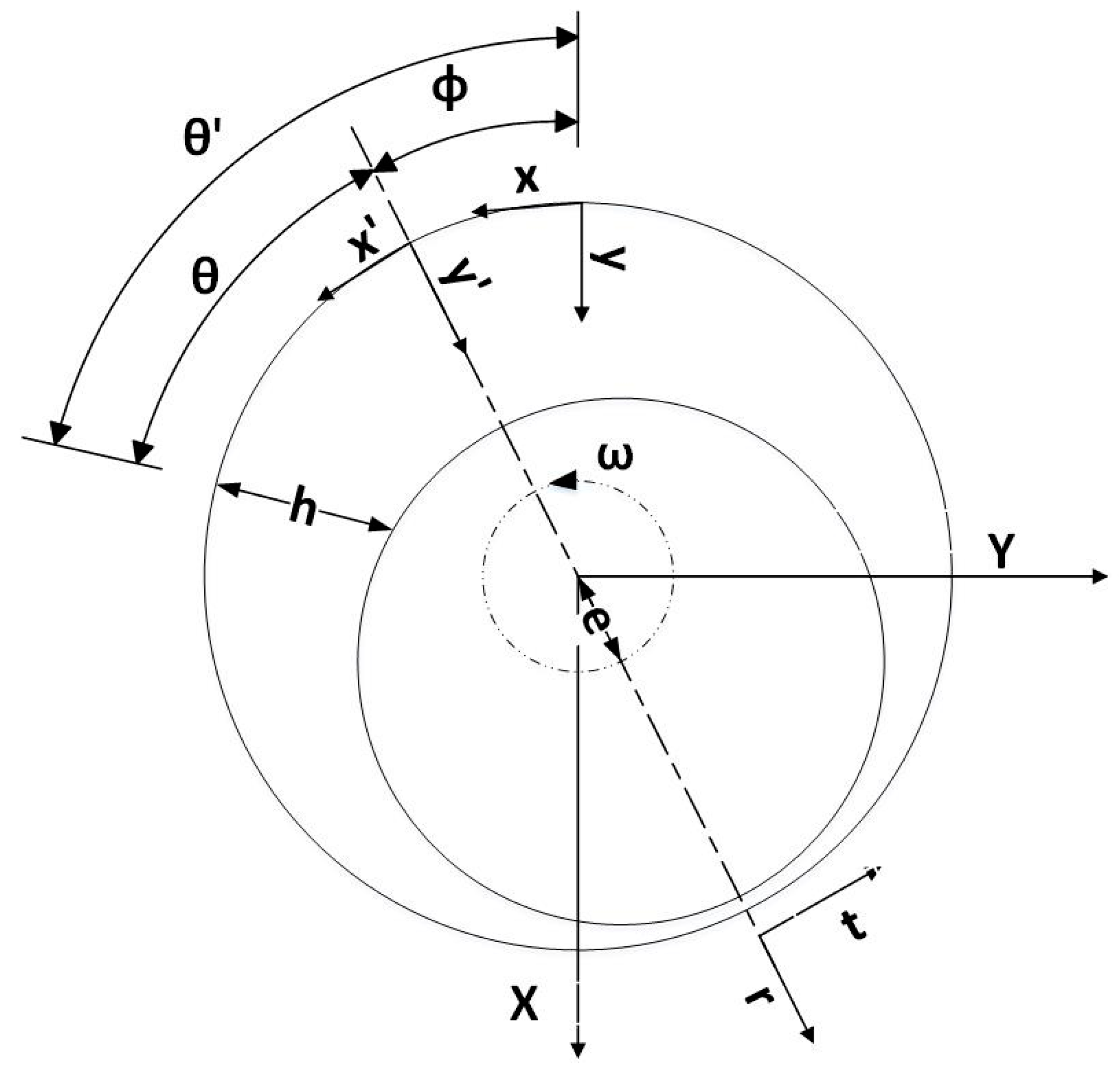
Figure 3.
The effect of fluid inertia at small eccentricity ratios on the midplane pressure distribution. (a) ; (b) ; (c) ; and (d) .
Figure 3.
The effect of fluid inertia at small eccentricity ratios on the midplane pressure distribution. (a) ; (b) ; (c) ; and (d) .

Figure 4.
The effect of fluid inertia at moderate eccentricity ratios on the midplane pressure distribution. (a) ; (b) ; (c) ; and (d) .
Figure 4.
The effect of fluid inertia at moderate eccentricity ratios on the midplane pressure distribution. (a) ; (b) ; (c) ; and (d) .


Figure 5.
The effect of fluid inertia at large eccentricity ratios on the midplane pressure distribution. (a) ; (b) ; (c) ; and (d) .
Figure 5.
The effect of fluid inertia at large eccentricity ratios on the midplane pressure distribution. (a) ; (b) ; (c) ; and (d) .
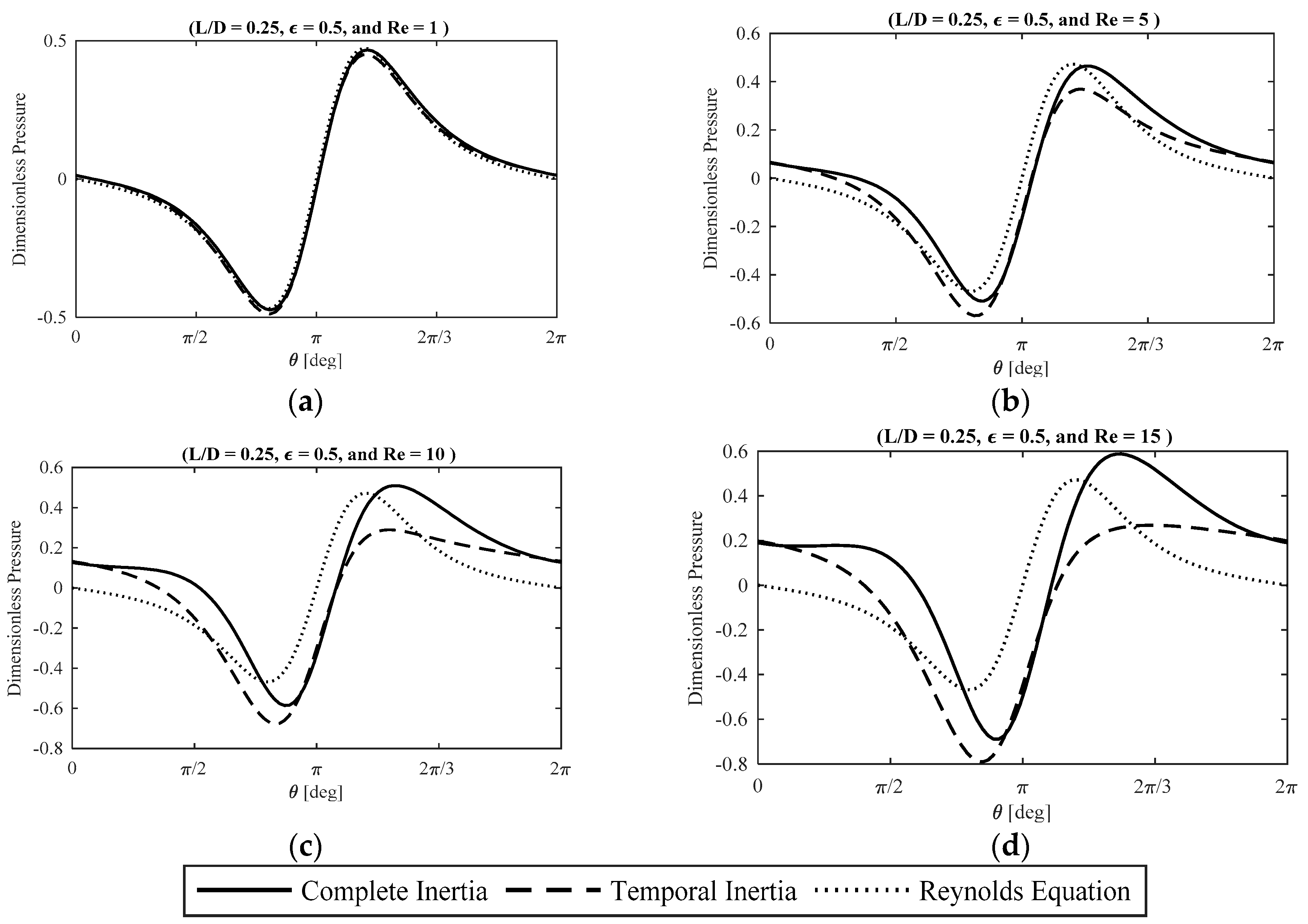
Figure 6.
The effect of fluid inertia on the fluid film force components. (a) at ; (b) at ; (c) at ; (d) at ; (e) at ; (f) at ; (g) at ; (h) at ; (i) at ; and (j) at .
Figure 6.
The effect of fluid inertia on the fluid film force components. (a) at ; (b) at ; (c) at ; (d) at ; (e) at ; (f) at ; (g) at ; (h) at ; (i) at ; and (j) at .
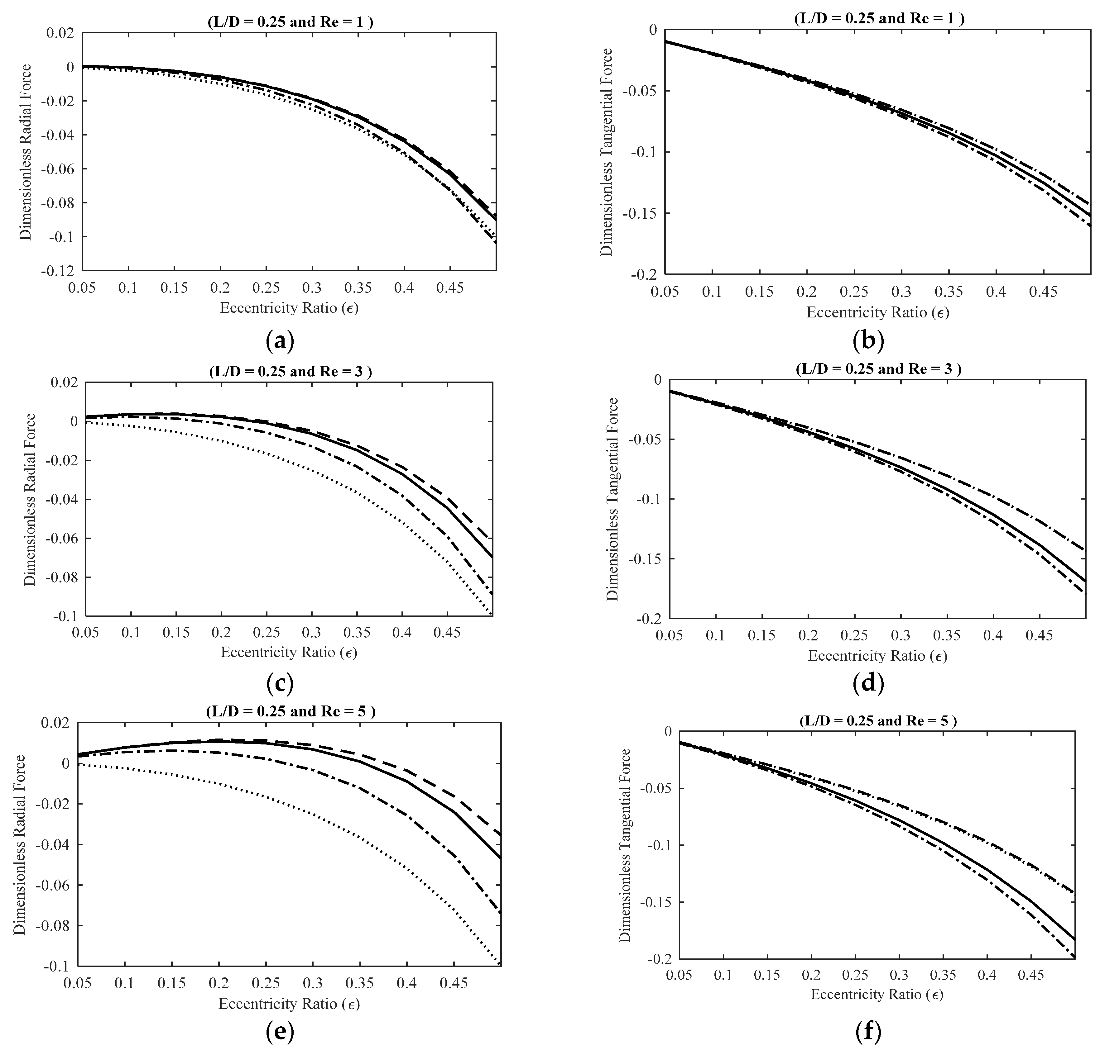

Figure 7.
The modal integration algorithm with predictor–corrector solver.
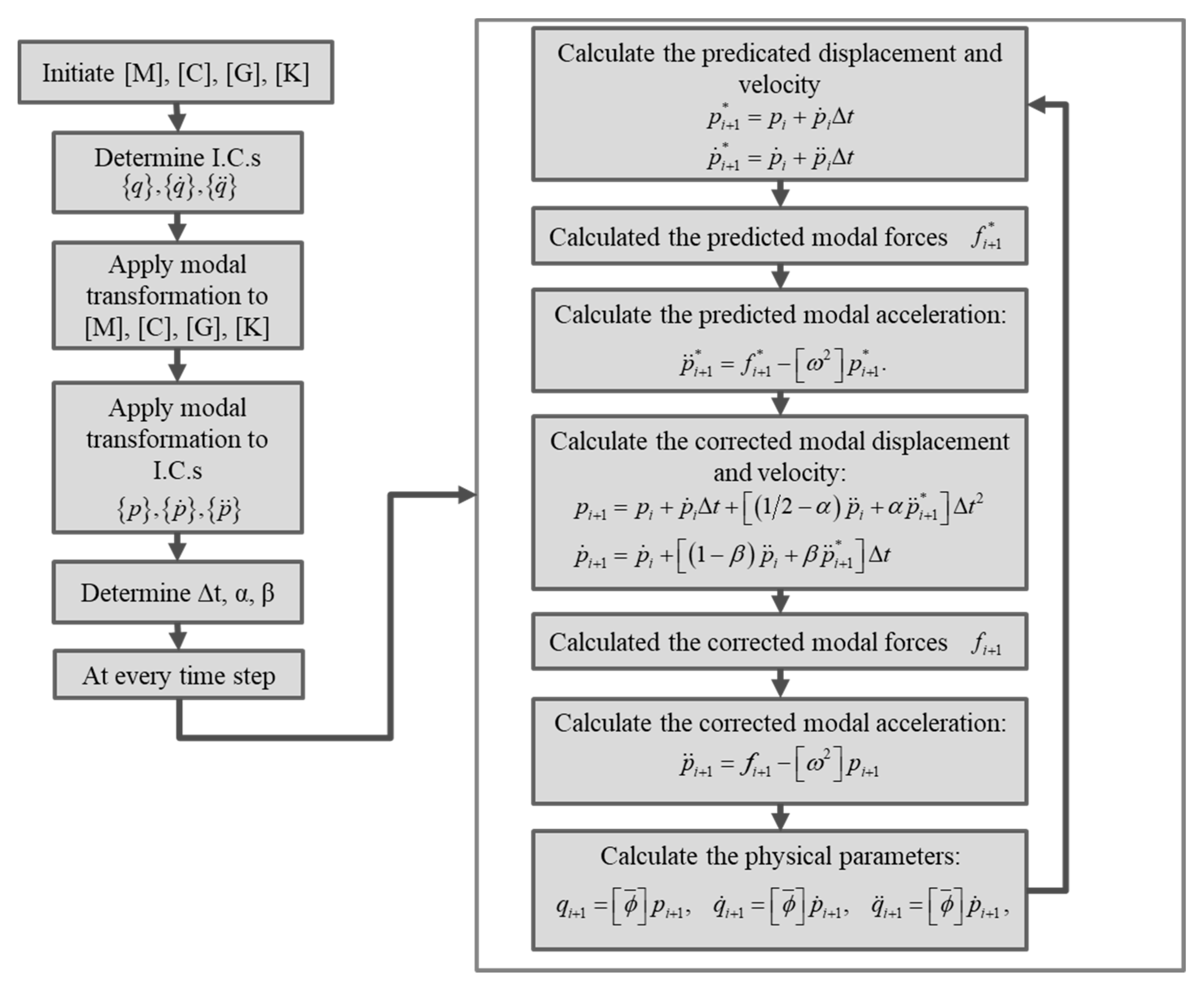
Figure 8.
The rotor system schematic in the simulation model.
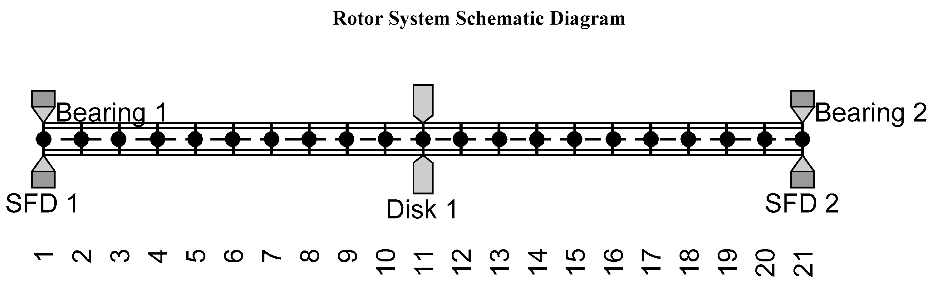
Figure 9.
The effect of SFD on the steady-state vibration amplitudes of the rotor system. (a) Unbalance magnitude 7.2008 × 10⁻⁵; (b) Unbalance magnitude 1.4402 × 10⁻⁴; and (c) Unbalance Magnitude 3.6004 × 10⁻⁴.
Figure 9.
The effect of SFD on the steady-state vibration amplitudes of the rotor system. (a) Unbalance magnitude 7.2008 × 10⁻⁵; (b) Unbalance magnitude 1.4402 × 10⁻⁴; and (c) Unbalance Magnitude 3.6004 × 10⁻⁴.
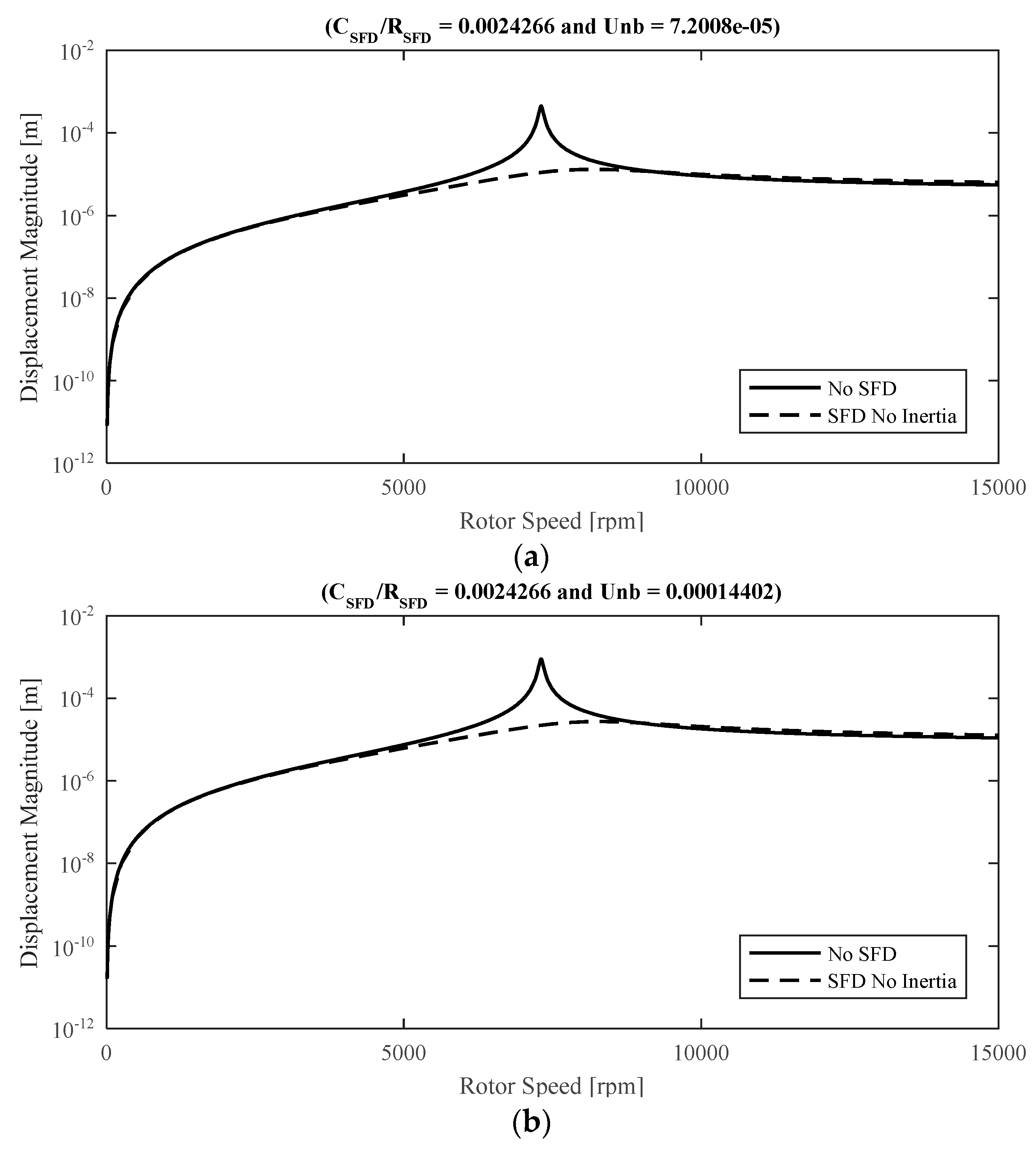
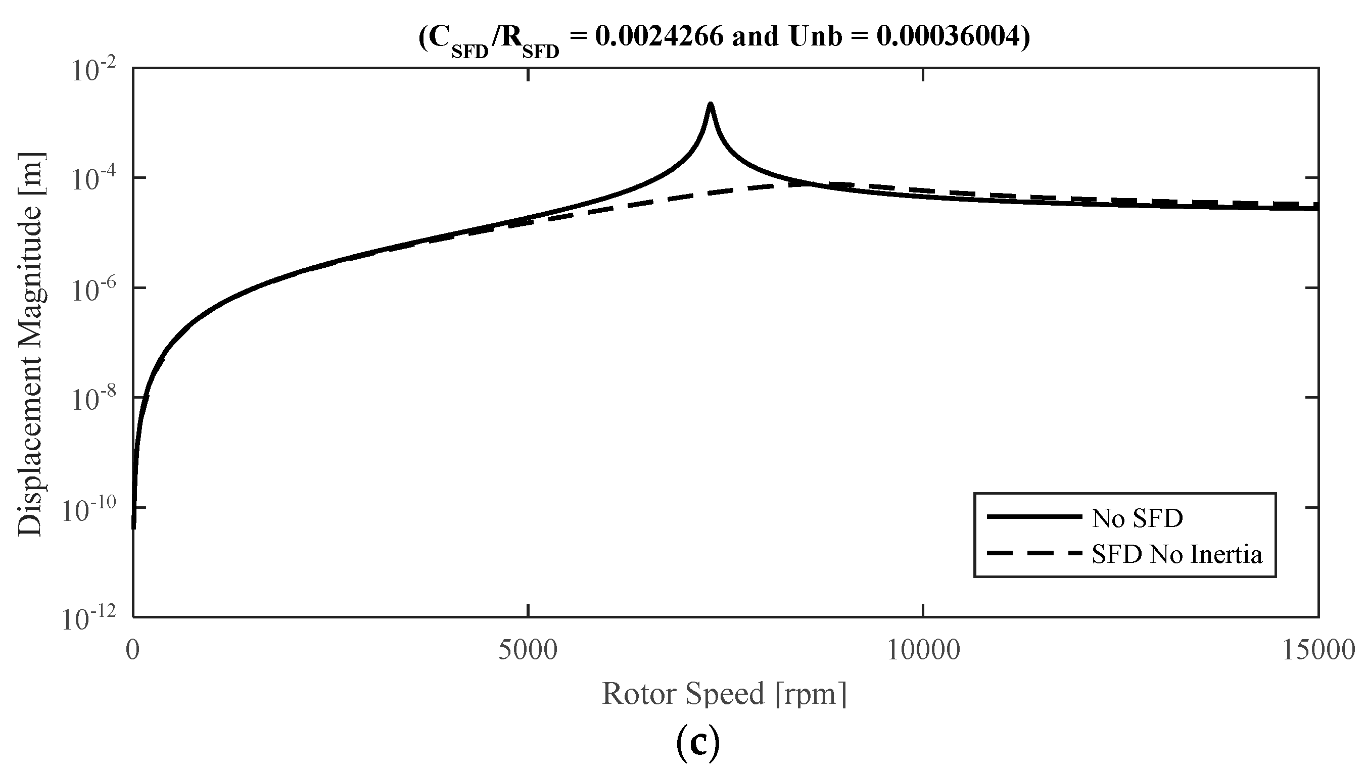
Figure 10.
The effect of SFD lubricant inertia on the steady-state vibration amplitudes of the rotor system. (a) Unbalance magnitude 7.2008 × 10⁻⁵; (b) Unbalance magnitude 1.4402 × 10⁻⁴; and (c) Unbalance Magnitude 3.6004 × 10⁻⁴.
Figure 10.
The effect of SFD lubricant inertia on the steady-state vibration amplitudes of the rotor system. (a) Unbalance magnitude 7.2008 × 10⁻⁵; (b) Unbalance magnitude 1.4402 × 10⁻⁴; and (c) Unbalance Magnitude 3.6004 × 10⁻⁴.


Figure 11.
The transient orbit radius of the SFD journal center at different rotor speeds.


Table 1.
The rotor system parameters.
| Parameter | Value | Unit |
|---|---|---|
| c11, c22 | 175.1268 | N·s/m |
| c12, c21 | 0 | N·s/m |
| 0.00242 | ||
| Dout, Din | 0.0603 and 0.0413 | m |
| Dd,out, Dd,in | 0.2032 and 0.0603 | m |
| D | 0.1047 | m |
| Ee | 2.11 × 10¹¹ | pa |
| Gshear,e | 8.1783 × 10¹⁰ | pa |
| k11, k22 | 8.7563 × 10⁶ | N/m |
| k12, k21 | 0 | N/m |
| Lshaft | 0.5994 | m |
| 0.325 | ||
| munbσ | 3.6004 × 10⁻⁴, 1.4402 × 10⁻⁴, 7.2008 × 10⁻⁵ | kg·m |
| Wd | 0.0508 | m |
| α, β | 0.5 and 0.25 | |
| μ | 0.0051 at 100 °C | Pa·s |
| ρe | 7810 | kg/m3 |
| ρd | 7810 | kg/m3 |
| ρ | 1003.5 | kg/m3 |
| 0.29 | ||
| Ω | 100 to 15,000 | rpm |
| Δt | 10−5 | s |
© 2017 by the authors. Licensee MDPI, Basel, Switzerland. This article is an open access article distributed under the terms and conditions of the Creative Commons Attribution (CC BY) license (http://creativecommons.org/licenses/by/4.0/).
Share and Cite
MDPI and ACS Style
Hamzehlouia, S.; Behdinan, K. A Study of Lubricant Inertia Effects for Squeeze Film Dampers Incorporated into High-Speed Turbomachinery. Lubricants 2017, 5, 43. https://doi.org/10.3390/lubricants5040043
AMA Style
Hamzehlouia S, Behdinan K. A Study of Lubricant Inertia Effects for Squeeze Film Dampers Incorporated into High-Speed Turbomachinery. Lubricants. 2017; 5(4):43. https://doi.org/10.3390/lubricants5040043
Chicago/Turabian StyleHamzehlouia, Sina, and Kamran Behdinan. 2017. "A Study of Lubricant Inertia Effects for Squeeze Film Dampers Incorporated into High-Speed Turbomachinery" Lubricants 5, no. 4: 43. https://doi.org/10.3390/lubricants5040043
Note that from the first issue of 2016, this journal uses article numbers instead of page numbers. See further details here.