EHD Effects in Lubricated Journal Bearing

Department Cathedra of high mathematics 2, National Research University of Electronic Technology, 124498 Zelenograd, Moscow, Russia
Lubricants 2018, 6(1), 12; https://doi.org/10.3390/lubricants6010012
Submission received: 30 October 2017
/
Revised: 16 January 2018
/
Accepted: 16 January 2018
/
Published: 23 January 2018
(This article belongs to the Special Issue Friction and Lubrication of Sliding Bearings)
Abstract
:This paper presents a numerical analysis of the influence of deformation of infinite parallel cylindrical solids in partial journal bearing on the oil film characteristics. The stationary elastohydrodynamic EHD problems for three design models of bearings are considered: (1) The bearing in which the basic contribution to the elastic displacement of the surface brings the thin elastic liner; (2) The elastic cylinder and the elastic bushing which is modeled by the elastic space with a cylindrical cut; (3) The elastic cylinder and the elastic bushing in the presence of the thin elastic liner with a small module of elasticity. It is shown that when the minimum film thickness is fixed and deformations of the elastic solids increase, then the load capacity increases, reaches a maximum, and then decreases. The deformation of solids can raise load capacity many times over. When the deformation of solids increases from zero, the pressure distribution changes from the distribution of pressure in the case of rigid bodies to the distribution of pressure which takes place with the dry contact of elastic bodies.
1. Introduction
Nowadays, most hydrodynamic journal bearings are required to operate with decreasing film thicknesses. When a bearing is highly loaded, the elastic displacements can exceed the minimum film thickness and can essentially influence the bearing characteristics.
The deformation effects on the characteristics of a plain journal bearing have been studied in a number of works. Higginson [1] and Angra et al. [2] presented an analysis of the effects of the elastic deformation of the bearing liner on the performance of a journal bearing. The calculations were made at high values of the minimum film thickness. The results of the calculations show that at a fixed minimum film thickness the load grows as the liner becomes more flexible, but this growth is not great.
An analysis of the EHD behavior of a bearing operating under conditions which tend to be severe was presented by Bendaoudl et al. [3]. The influence of mechanical deformations were presented at one load. It was shown that the minimum film thickness was 18% less when deformations were not taken into account in the calculations.
The significance of the deformation effects on a plane journal bearing subjected to severe operating conditions was studied by Bouyer et al. [4]. It was shown that mechanical deformations significantly decrease the maximum pressure, significantly modify the profile of the lubricant gap, but do not have a great influence on the minimum film thickness magnitude. These conclusions were made on a basis of the analysis of the results of calculations for two loads.
Chetti [5] and Osman [6] studied the load dependence on eccentricity for rigid bodies and deformable bodies. The obtained results for elastic bearings was lower than those for rigid bearings for the whole range of eccentricity.
In all previous work the solutions were proposed only for several loads and for large minimum film thicknesses. They do not give a representation of how mechanical deformations influence the characteristics of a lubricant layer in the transition from small deformations to big deformations.
In the present work, a numerical analysis of the influence of deformations of infinite parallel cylindrical solids in partial journal bearings on the oil film characteristics is presented. It is shown that when the minimum film thickness is fixed and the deformation of the elastic solid increases, then the load capacity increases, reaches a maximum, and then decreases. The deformation of solids can raise the load capacity many times over.
2. Design Model One
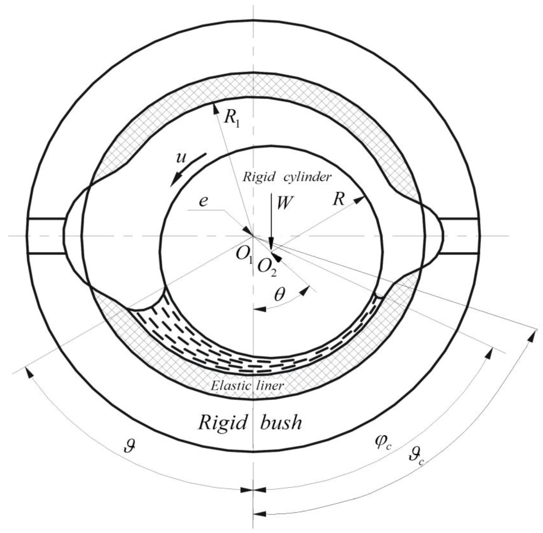
Let us consider the conformal contact of a hard shaft and thin elastic liner that is inserted into a rigid bush (Figure 1). The inner radius of the liner is a little different from the radius of the shaft , which is , where , is the inner radius of the liner.
Let the line of center (Figure 1) of the bearing and shaft form with the line of action of the load angle , which is defined when solving the problem. The angular coordinate is measured from the line of action of the load in the direction of movement of the surface of the shaft.
Consider the case of a partial journal bearing. In this case, the inlet coordinate of a lubricant layer is determined by the position of the input oil-groove, from which the oil arrives under slight pressure into the gap. Then the inlet coordinate of a lubricant layer is equal to . The coordinate of the output point of a lubricant layer is unknown and is determined when solving the problem. This coordinate should satisfy the condition . Here is the coordinate of the inlet boundary of the output oil-groove in which the lubricant arrives after passing the zone of high pressure.
If condition (1) is satisfied, then the deformation of the shaft and bush can be neglected when determining the film thickness, and only the deformation of the liner must be taken into account.
Here is the thickness of the liner, and are the elastic modules of liner, shaft and bush respectively.
The elastic displacement of the shaft surface is proportional of the shaft radius and inversely proportional to the modulus of elasticity of the shaft , that is . The elastic displacement of the bush surface is and the elastic displacement of the liner surface is . Here and are some constants. The conditions (1) follow from these expressions and from the conditions and .
When the additional condition is correct, then the displacement of the liner surface can be defined as [7,8]
Here is pressure which acts from the lubricant layer to the surface of the liner, and is the Poisson’s ratio of liner. According to (2), the film thickness can be defined as:
Here is the eccentricity. The pressure we define from the Reynolds equation
Here and are the oil density and viscosity respectively, and is the velocity. The oil density and viscosity depend on the pressure as follows
Here and are the oil density and viscosity at atmospheric pressure respectively, and are constant and is pressure coefficient of viscosity.
The boundary conditions for the pressure are of the form
Condition (5) means that if is obtained when using the condition then it is necessary to accept and to solve the problem without using the condition In this paper we will suppose that the angles and are such that the condition is satisfied. Integrating Equation (3) in the domain and taking into account boundary condition (5), the following equation can be obtained
The conditions of the balance of forces look like
Here is the force, and is tangent stress acting from a lubricant layer on a shaft.
The following dimensionless variables are defined
Here is characteristic elastic contact pressure. When the displacement of the liner surface equals the radial clearance .
In dimensionless variables, the equations and conditions can be represented as follows
Here , is relative eccentricity
is the characteristic hydrodynamic pressure, , , , and is dimensionless force which is equal to
Dimensionless parameter equals the ratio of the characteristic hydrodynamic pressure to the characteristic elastic contact pressure. When this parameter is small the pressure is also small compared to characteristic elastic contact pressure, and deformations of the liner have little effect on the solution of the problem. It means that at small values for parameter the solution of the problem differs slightly from the solution for rigid bodies. When parameter increases, the influence of the deformations of the liner on the pressure and film thickness also increases.
2.1. Asymptotic Properties of the Solution
Let us consider the solution of the problem at large values of parameter and when the influence of pressure on lubricant density and viscosity is not taken into account, that is at , . It follows from (7) that in this case
Since the pressure and pressure derivative are limited then
It follows from (6) and (14) that at where
Let us consider the case when and . The angle is proportional to when function looks like (15). Parameter is usually small and we can accept . It is not difficult to obtain in this case
2.2. Numerical Method
The input parameters of the problem are and . After setting these parameters, the functions , , and parameters and can be found by solving the system of Equations (6)–(8) under conditions (9) and (11). The dimensionless load can be found using the expression (10) after that.
The angles are defined by iteration. The initial approach of these parameters is assigned at first. Thus, the initial values of are specified before the calculations.
The mesh of nodes , , , is entered. It follows from Equations (6)–(8), that
Equations (9) and (10) can be presented as (24) and (25) after replacing the integrals by finite sum.
As and are known, we can calculate on Formula (18) and on Formula (20). The condition must be taken into account. As are known, the value of can be found using the Equation (22) and expressions (23). Really, after substitution of expression (23) into the Equation (22) and the assignment of , we receive a non-linear equation with respect to . After solving this equation, the values of and can be defined under the Formulas (19) and (21).
Further, the value of can be calculated and so on. As a result, the values of and can be calculated consistently at . Thus, the values of and can be calculated if the values of are assigned. After that can be computed on Formulas (26), (27) and parameter can be determined.
The validity of the conditions (28) indicates that the solution of the problem is found.
Here and are the parameters which determine the precision of the solution. They are set before the calculations.
The flowchart for determining and is shown in Figure 2. Equation (22) is solved with respect to using Newton iterations.
The number of nodes determines the accuracy of the solution. The influence of number on the accuracy of the solution is illustrated by the results of the calculation presented in Table 1. The calculation was made at the next values of parameter: , , , , .
The results in Table 1 indicate that the results of the calculation have high precision when .
2.3. Discussion
At first, we will consider the results when the influence of pressure on lubricant density and viscosity is not taken into account, that is, the decision of a problem at . Figure 3, Figure 4, Figure 5 and Figure 6 present the results at radians.
The ratio (29) is proportional to the dimension load and does not depend on the elastic properties of the liner. The parameter is inversely proportional to the modulus of elasticity of the liner. Therefore, the dependence of ratio on parameter characterizes the influence of the elasticity of the liner on the load.
Chetti [5] and Osman [6] presented the dependence of load from eccentricity for rigid bodies and deformable bodies. They came to the conclusion that at given eccentricities the load for rigid bearing is greater than that for elastic bearing.
Figure 3 shows the dependences of ratio and minimum film thickness on at . It follows from these results that the dimension load decreases when the elastic deformation of the liner increases as in [5,6]. However, the presented results also demonstrate that at a given eccentricity the minimum film thickness essentially increases when the elastic deformation increases. This means that the influence of deformations on the film thickness may be shown more demonstrably by the dependences of the ratio on at .
Figure 4 shows the dependences of on at different values of . When then the solution of the problem approaches the solution for the rigid bodies. Therefore
Here is the load in a pure hydrodynamic regime which depends on the minimum film thickness, that is .
The value of coordinate does not exceed the value of in all the presented results of the calculation. The pressure distribution approaches the pressure distribution for the dry contact of a rigid cylinder and an elastic liner at a large value of . It follows from (17) that at and a large value of there will be
Relationship (30) is presented in Figure 4 as a linear dependence.
It follows from the results presented in Figure 4 that the ratio as a function of has a maximum. When the deformations of the liner are small, they lead to an increase in the load capacity of the lubricant layer. However, when the deformations of the liner are large, they can decrease this load capacity.
The elasticity of the liner can raise the load capacity of the lubricant layer many times over. For example, at this increase can be 18 times. At this increase may not be more than two times.
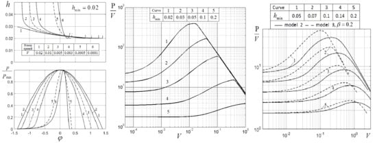
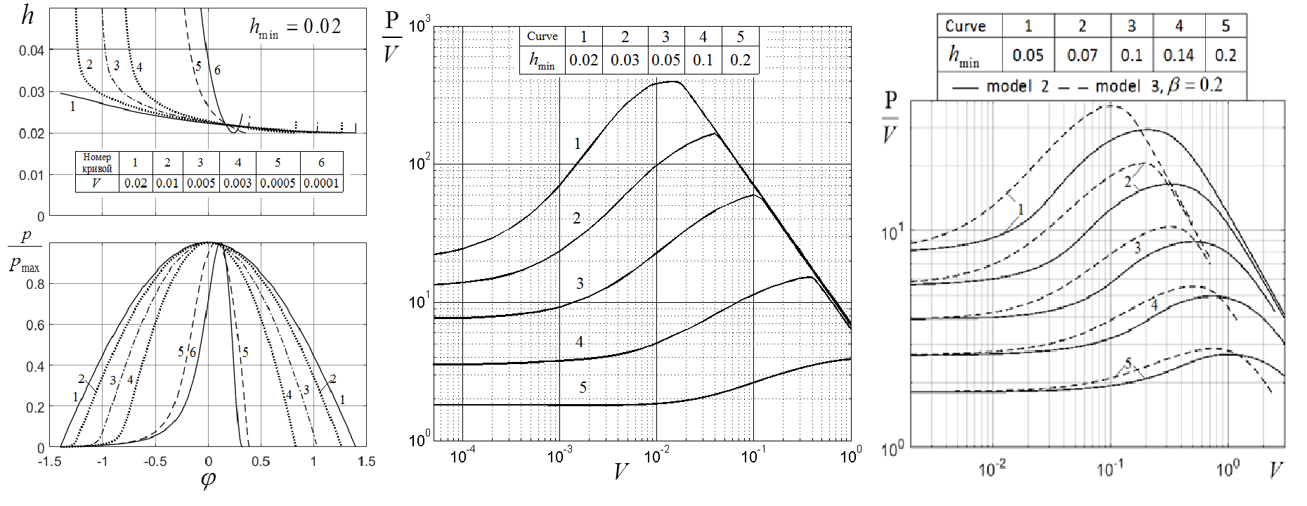
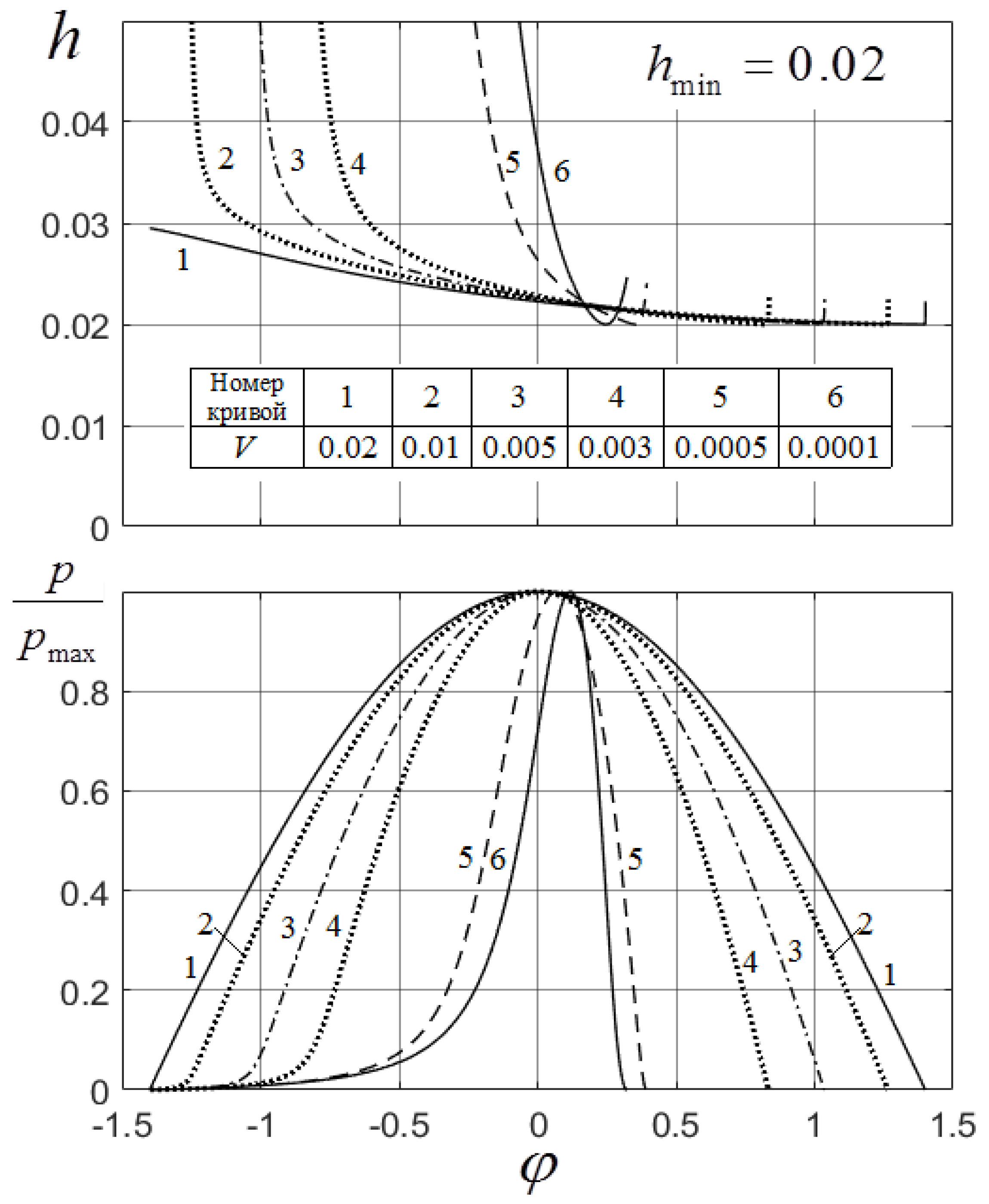
Figure 5 shows the dependences of and at various values of parameter and at . It follows from these results that the point of minimum function moves to the left when increases. The pressure distribution gradually passes from specific hydrodynamic distribution to pressure distribution in dry contact.
Higher values of parameter correspond to a more flexible liner. The shaft penetrates into the liner more deeply if the liner is more flexible. This leads to an increase of the size of the contact zone when parameter increases. The point of minimum film thickness was located near the output point of a lubricating layer. As a result, the point of minimum film thickness shifts towards right as parameter increases.
Figure 6 shows the dependences of the maximum of pressure on parameter at different values of . It follows from these results that the dependence of on is close to linear dependence up to the limiting value
The results presented above are received without taking into account the influence of oil density and viscosity variation. This influence is illustrated by the curves in Figure 7.
Figure 7 shows the dependences of ratio on at . Curve 1 is obtained when the influence of oil density and viscosity variation are not taken into account. Curve 4 presents results when only the influence of the viscosity variation is taken into account. Curve 2 presents results when only the influence of density variation is taken into account. Curve 3 presents results when the influence of density and viscosity variations is taken into account.
The presented results indicate that the density variation with the variation of pressure leads to a small variation in the load capacity of the lubricant layer. Basically, this influence becomes appreciable only in a small vicinity of the value of at which the function has a maximum.
The influence of the viscosity variation on load capacity also is small and it also is maximal in a small vicinity of the value of at which the function has a maximum. However, the influence of viscosity variation on load capacity is more important than the influence of density variation, because curves 3 and 4 are quite close to each other compared to curves 1 and 2.
3. Design Model Two
Now we will determine the deformation of the elastic shaft and elastic bushing using the solution of the plane problem of theory elasticity for the elastic circle and for the elastic plane with circular cut.
A general solution to the problem of elasticity for circular rings is given in a book [9]. It follows from this solution that the elastic displacement of the surface of elastic circles can be determined under the formula
Here and are constants that must be specified when solving a specific problem,
The elastic displacement of the surface of the circular cut in elastic plane can be determined under the formula
Let us consider the case of and . Taking into account the expression (31) and (32), the film thickness can be determined under the formula
The following dimensionless variables are defined
In dimensionless form the basic equations look like
Here
3.1. Numerical Method
When calculating the value of at the mesh point , the function is approximated by a piecewise linear function (43)
where .
Substituting (43) into (35) and using the integrals (44), (45) the expression (46) can be obtained
The Reynolds’s Equation (36) can be written in the finite difference form as
The conditions of the balance of forces looks like in the case of mathematical model 1.
The variable and can be excluded from Equation (47) by using expressions (23) and (46). As a result, these equations will represent the system of equations with respect to variables . This system of equations together with the equation of balance of forces defines the variables and the variable . The specified system of equations is solved using the Newton iterations method.
3.2. Discussion
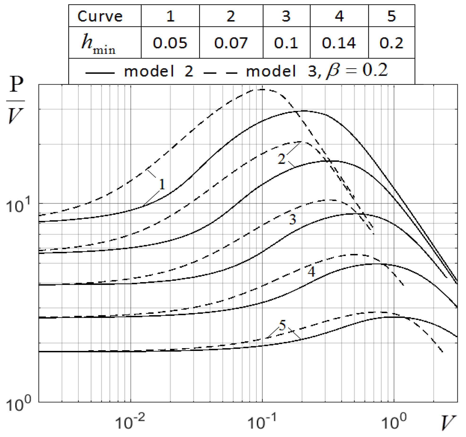
Figure 8 presents results that are analogous to the results presented in previous section. The calculation where made at and . The solid curves present the results of the calculation of the discussed design model two. The dashed curves present the results of calculation of design model three, which will be discussed later.
The presented results indicate that the solution of this problem has the same properties as the solution of the problem for bearings with a thin liner. In particular, the function has a maximum which shifts to the right with the growth of . The growth of the load capacity of the lubricant layer caused by the deformation of bodies can be more than in 3.5 times when . This growth can reach values of 1.5 when .
The calculations indicate that as in the case of model one, variation of the viscosity and density of the lubricant slightly influences film thickness and pressure.
4. Design Model Three
It follows from the results presented above that deformations can essentially raise the load capacity of a lubricant layer. The maximum load capacity is provided at a certain value of parameter which looks like (12) in a bearing with a thin liner when the shaft and bush deformations can be neglected, and looks like (41) in the case of a homogeneous elastic shaft and a homogeneous elastic bush.
If the bearing is projected on a certain regime it is desirable to pick up the parameters so that the deformations as much as possible raise the loading capacity of the bearing. However, if materials with the specified module of elasticity are used and the specified lubricant is used, then there are a few possibilities to obtain a maximal load capacity by changing the value of parameter . However, there is a possibility of increasing the load at the expense of the deformation of bodies by the introduction of the thin elastic liner with a small module of elasticity.
The given circumstance is illustrated by the results of the calculations for the scheme presented in Figure 9. The results of the calculations for this bearing scheme are shown in Figure 8.
The scheme of the bearing consists of an elastic shaft, elastic bush end elastic thin liner, the modules elasticity of which is small. In this case the film thickness can be defined as
Here are the Poisson’s coefficient and module elasticity of liner, respectively. In dimensionless variables defined as (34), the Equation (48) looks like
where .
The value of corresponds to the case , that is, the case when the elastic liner is absent. The increase of parameter corresponds to the increase in the liner thickness.
The dashed curves in Figure 8 show the dependences of the function at different values of and at . The results presented in Figure 8 indicate that the thin liner leads to an increase in the maximum bearing load capacity and leads to a decrease in the value of parameter at which the function has a maximum.
5. Example of Bearing Calculation
Determine the minimum film thickness of the bearing mill roll, the construction of which corresponds to design model two. The parameters of the bearing are: , , , , , , , , .
According to the Formulas (34), (41) and (42) we find , , and . These values of and correspond to points in Figure 8, which is between the curves and . The calculations indicate that at these values of and correspond to and .
It follows from the results of the calculation that when and then and . This means that the deformation increased the load capacity more than two times.
Consider the influence of the viscosity variation on the minimum film thickness. Using (42) we have . It follows from the solution of system of equation that and at this value of and at . Thus the increase in lubricant viscosity leads to an increase in minimum film thickness of 13.7 percent.
Consider the influence of density variation on minimum film thickness. Using (42), we have . The calculations give and at these values of parameters and at . Thus the increase in lubricant density leads to an increase in minimum film thickness of 0.6 percent.
6. Conclusions
The stationary EHD problems for three design models of bearings were considered:
- (1)
- The bearing in which the basic contribution to the deformation brings a thin elastic liner;
- (2)
- The elastic cylinder and the elastic bushing, which is modeled by an elastic space with a cylindrical cut;
- (3)
- The elastic cylinder and the elastic bushing in the presence of a thin elastic liner with a small module of elasticity.
It was shown that when the minimum film thickness is fixed and the deformations of the elastic solids increase, then the load capacity increases, reaches a maximum, and then decreases. Deformations of solids can raise load capacity many times over.
The maximum load capacity takes place at a certain value of dimensionless parameters which is proportional to the speed, the lubricant viscosity and inversely proportional to the elasticity module. It was shown that the presence of the thin elastic liner in the third settlement scheme of the bearing led to a reduction of the value of the dimensionless parameters at which the load capacity has a maximum. This means that it is possible to essentially raise the load capacity of bearings at operating conditions by the introduction of a liner with a small module of elasticity.
When the deformations of solids increase from zero, the pressure distribution changes from the distribution of pressure in the case of rigid bodies to the distribution of pressure that takes place in the dry contact of elastic bodies.
Conflicts of Interest
The author declares no conflict of interest.
References
- Higginson, G.R. The Theoretical Effects of Elastic Deformation of the Bearing Liner on Journal Bearings Performance. In Proceedings of the Symposium on Elastohydrodynamic Lubrication; Institution of Mechanical Engineers: Westminster, UK, 1965; Volume 180, pp. 31–38. [Google Scholar]
- Angra, S.; Mehta, N.P.; Rattan, S.S. Effects of elastic deformation of bearing liner on performance of finite offset-halves pressure dam bearings. Tribol. Lett. 1996, 2, 273–285. [Google Scholar] [CrossRef]
- Bendaoud, N.; Mehala, K.; Youcefi, A.; Fillon, M. An experimental and numerical investigation in elastohydrodynamic behaviour of a plain cylindrical journal bearing heavily loaded. Proc. Inst. Mech. Eng. J. 2012, 226, 809–818. [Google Scholar] [CrossRef]
- Bouyer, J.; Fillon, M. On the Significance of Thermal and Deformation Effects on a Plain Journal Bearing Subjected to Severe Operating Condition. J. Tribol. 2004, 126, 819–822. [Google Scholar] [CrossRef]
- Chetti, B. Analysis of a circular journal bearing lubricated with micropolar fluids including EHD effect. Ind. Lubr. Tribol. 2014, 66, 168–173. [Google Scholar] [CrossRef]
- Osman, T.A. Effect of lubricant non-Newtonian behavior and elastic deformation on the dynamic performance of finite journal plastic bearing. Tribol. Lett. 2004, 17, 31–40. [Google Scholar] [CrossRef]
- Rades, M. Dynamic Analysis of an Inertial Foundation Model. Int. J. Solids Struct. 1972, 8, 1353–1372. [Google Scholar] [CrossRef]
- Lahmar, M.; Haddad, A.; Nicolas, D. Elastohydrodynamic analysis of one-layered journal bearings. Proc. Inst. Mech. Eng. 1998, 212, 193–205. [Google Scholar] [CrossRef]
- Galachov, M.A.; Usov, P.P. Differential and Integral Equations of Mathematical Theory of Lubrication; Nauka: Moscow, Russia, 1990; p. 290. [Google Scholar]
Figure 1.
Scheme of journal bearing. Rigid cylinder, rigid bush and elastic liner.

Figure 2.
Flowchart for determining and .
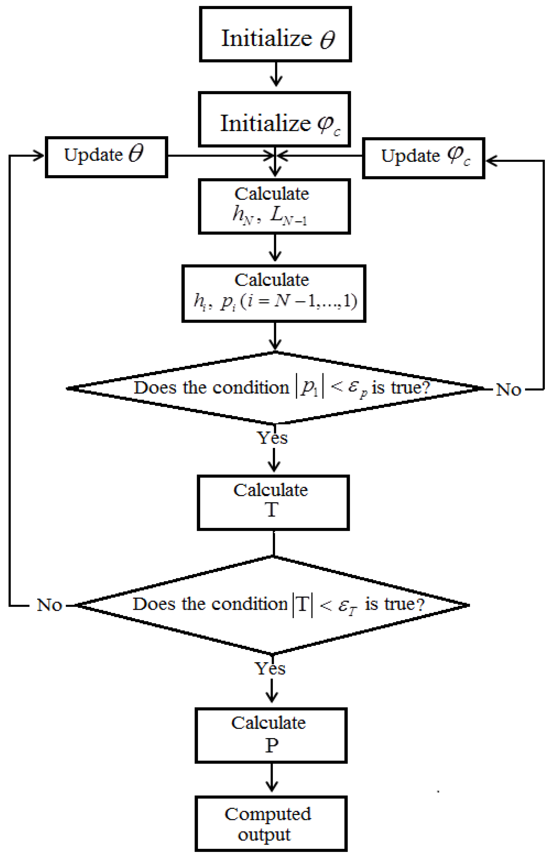
Figure 3.
Dependences of ratio and minimum film thickness on at .
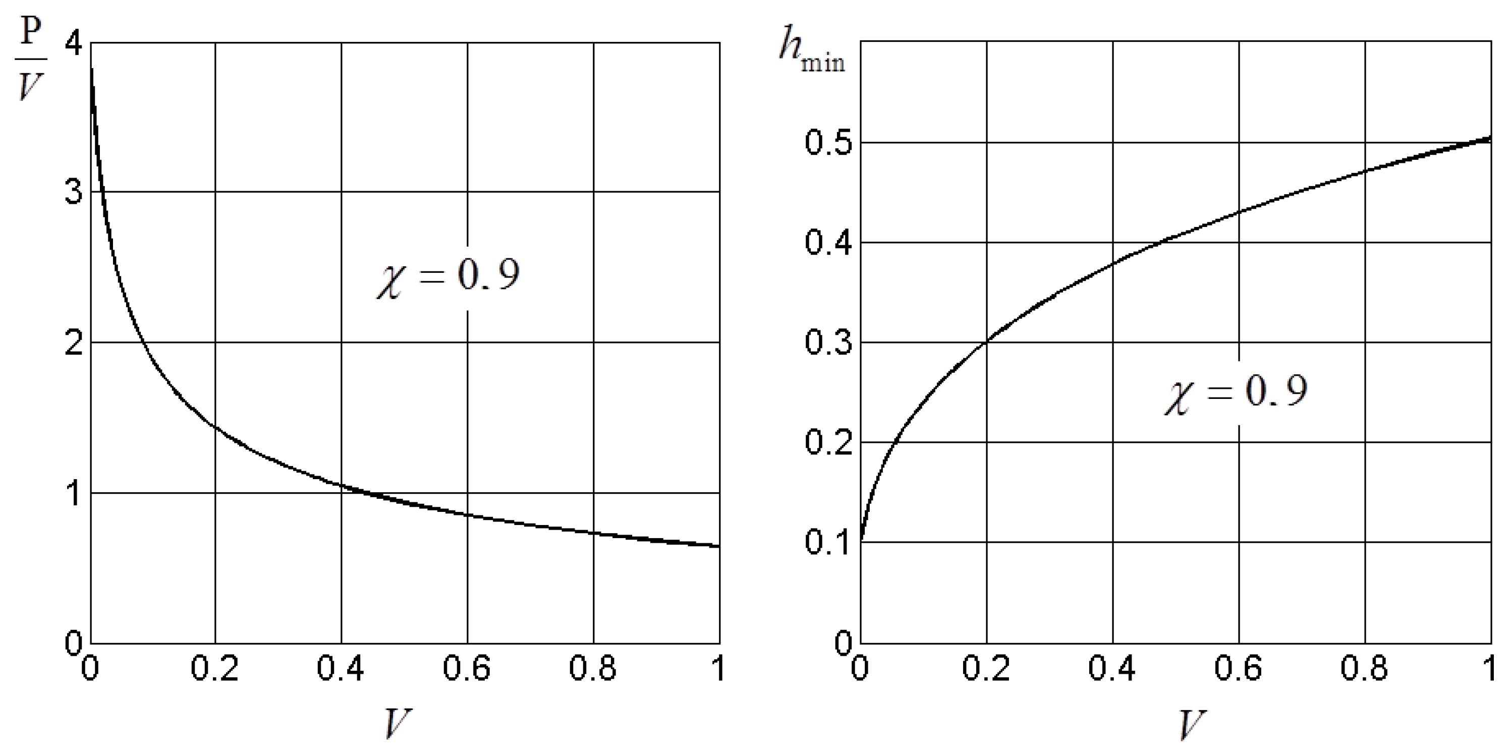
Figure 4.
Ratio as a function of at different values of .

Figure 5.
Dimensionless film thickness and ratio as a function of angle coordinate at and at different values of parameter .
Figure 5.
Dimensionless film thickness and ratio as a function of angle coordinate at and at different values of parameter .

Figure 6.
Dimensionless maximum pressure as a function of at and at different values of .

Figure 7.
Dependences of ratio on at .
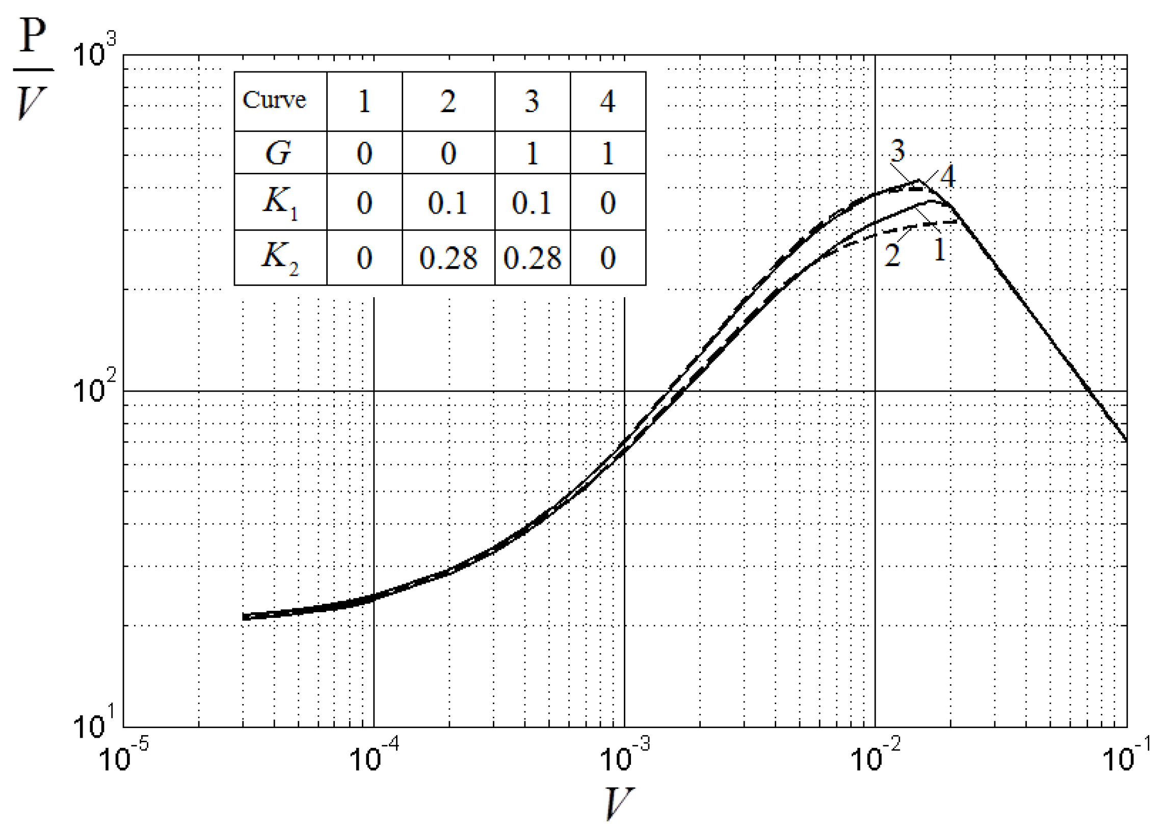
Figure 8.
Ratio as a function of at different values of .

Figure 9.
Scheme of journal bearing. Elastic cylinder, elastic bush and elastic liner.


Table 1.
The values of parameters and at various values of .
| 20 | 50 | 100 | 200 | 500 | |
| 0.33056 | 0.33585 | 0.33646 | 0.33660 | 0.33660 | |
| 0.04295 | 0.04312 | 0.04314 | 0.04315 | 0.04315 |
© 2018 by the author. Licensee MDPI, Basel, Switzerland. This article is an open access article distributed under the terms and conditions of the Creative Commons Attribution (CC BY) license (http://creativecommons.org/licenses/by/4.0/).
Share and Cite
MDPI and ACS Style
Usov, P.P. EHD Effects in Lubricated Journal Bearing. Lubricants 2018, 6, 12. https://doi.org/10.3390/lubricants6010012
AMA Style
Usov PP. EHD Effects in Lubricated Journal Bearing. Lubricants. 2018; 6(1):12. https://doi.org/10.3390/lubricants6010012
Chicago/Turabian StyleUsov, Pavel Pavlovich. 2018. "EHD Effects in Lubricated Journal Bearing" Lubricants 6, no. 1: 12. https://doi.org/10.3390/lubricants6010012
Note that from the first issue of 2016, this journal uses article numbers instead of page numbers. See further details here.