1. Introduction
In the aviation industry weight has always been a crucial question. On one hand, in order to reduce weight, one can find lightened gears, beams and lightened (hollow) shafts. On the other hand, these mechanical components should operate without excessive mechanical deformation which can lead to the damage of the machine.
Inside the accessory gearbox of a gas turbine, the power transmission is realized through gears mounted on a hollow shaft. In this case, the deformation of the shaft moves the gears out of their optimal functioning point. Since the gears are dimensioned and manufactured to operate at a given position, if they are moved out of this position, their wear increases and they may even break [
1,
2].
In order to limit the deflection of the shaft, a journal bearing might be mounted on the hollow shaft, close to the maximal deformation point. In the present study, a journal bearing was mounted close to the mid-point of a highly loaded hollow shaft, where the maximal deflection point is predicted. The journal bearing has a 30 wt % (mass fraction) carbon loaded PTFE ring under the bushing, while the bushing and the shaft are both made of structural steel. This study focuses on the behaviour of this journal bearing during the start-up period.
During start-up, the viscous forces in the oil film generate heat, which evacuates partially with the oil by convection and partially through the solids by conduction. Since the PTFE is a good thermal insulator (in other words has bad heat conduction coefficient), the bushing heats slower than the PTFE ring. On the contrary, the heating of the shaft generates thermal dilatation without any restriction. This means that the radial clearance of the journal bearing tends to decrease, resulting in a higher viscous shearing in the oil. The elevated viscous shearing transfers more heat to the solids, resulting in a faster closure of the radial clearance.
The clearance closure of a journal bearing was examined by Khonsari in 1989 [
3]. His study demonstrated the change of clearance during start-up. He found that the heating and dilation of the solids can close the clearance, which can be catastrophic for the journal bearing. In 1995, Pascovici published a numerical study [
4] on the characteristic time of radial clearance closure of a journal bearing. Pascovici found that there is a threshold at start-up that defines whether or not the clearance closure will occur. According to Pascovici [
4], the threshold depends on rotational speed, material, oil viscosity, radial clearance of the bearing and other parameters.
In 1998, Jang [
5] conducted friction torque measurements on a double axial groove journal bearing during start-up. The bearing bushing was made of glass and the bearing shaft was an epoxy resin. They compared their test results with THD analysis, which showed small discrepancies.
Kucinschi in 1999 and 2000 published the test results of a pseudo-transient hydrodynamic axial groove journal bearing at start-up [
6,
7]. Kucinschi observed several thermal phenomena in the bearing: the clearance closure between the bearing components, the response time of the bearing in case of acceleration or deceleration and the change of load carrying capacity. Their tests displayed a highly different behaviour in the case of a transitional regime than in the permanent cases. Kucinschi also measured the friction torque evolution during his experiments.
In 2011, Bouyer [
8] measured the friction torque during the start-up of an axial grooved plain journal bearing with a bronze bushing and a plain steel shaft. Bouyer varied the inlet temperature of oil during the tests, the radial load and the surface roughness of the shaft, but he did not continue his experiments until clearance closure.
Later, Cristea examined this phenomenon [
9] through a lumped model in case of circumferential groove journal bearing. Cristea found that for the same journal bearing in order to avoid seizure a rotational speed limit exists during start-up. Cristea [
9] found that for the same rotational speed a lower limit of radial clearance exists, which defines whether or not seizure will occur. Monmousseau [
10] published his pseudo-transient TEHD simulations for the case of a tilting pad journal bearing and he found a limit of acceleration rate for the occurrence of seizure during the start-up period.
Another transient phenomenon in the functionality of journal bearings is the cumulative wear: in 2016, Chun and Khonsari published a numerical study [
11] on rod bearing wear. They found that the roughness of the surfaces in contact and the direction and magnitude of the load changes the wear. In their studies, increasing the roughness of the surfaces in contact does not increase the wear in all cases: it is possible to reduce the wear by increasing the roughness, if the roughness of each of the two components is well chosen.
In our work, a test case for a circumferential groove journal bearing where the closure of the clearance results in seizure between the carbon-loaded PTFE ring and the steel shaft is revealed and discussed.
2. Presentation of the Test Bench
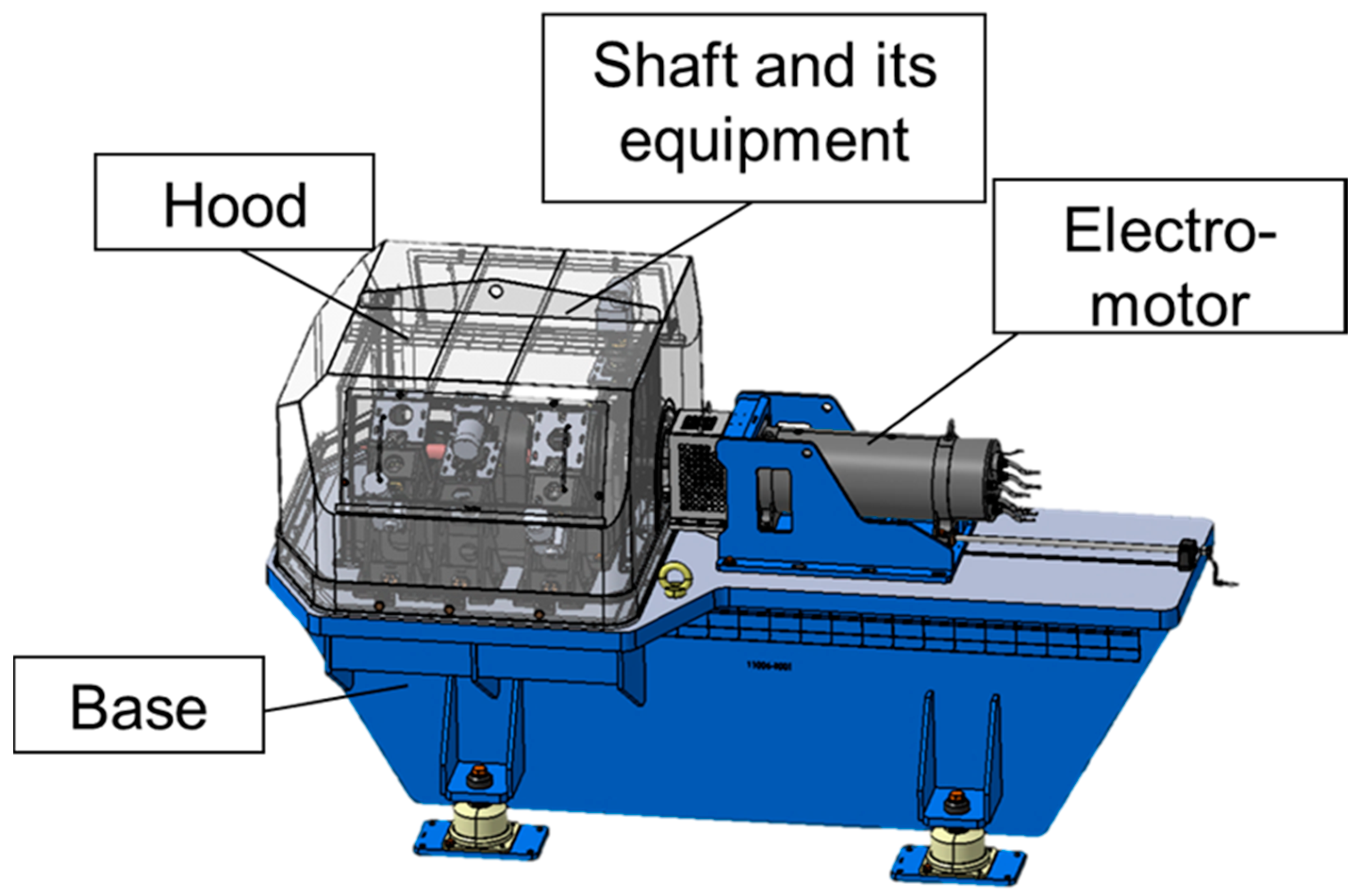
The experiments were realized on a test bench (
Figure 1), which was specifically developed for this purpose. The general and detailed description of the bench are presented in this section, with special emphasis on the instrumentation.
The symmetrical bushing mounted on the shaft is designed with a complete circumferential groove located in the journal bearing mid-plane. The geometrical parameters of the journal bearing and the lubricant oil properties are presented in
Table 1.
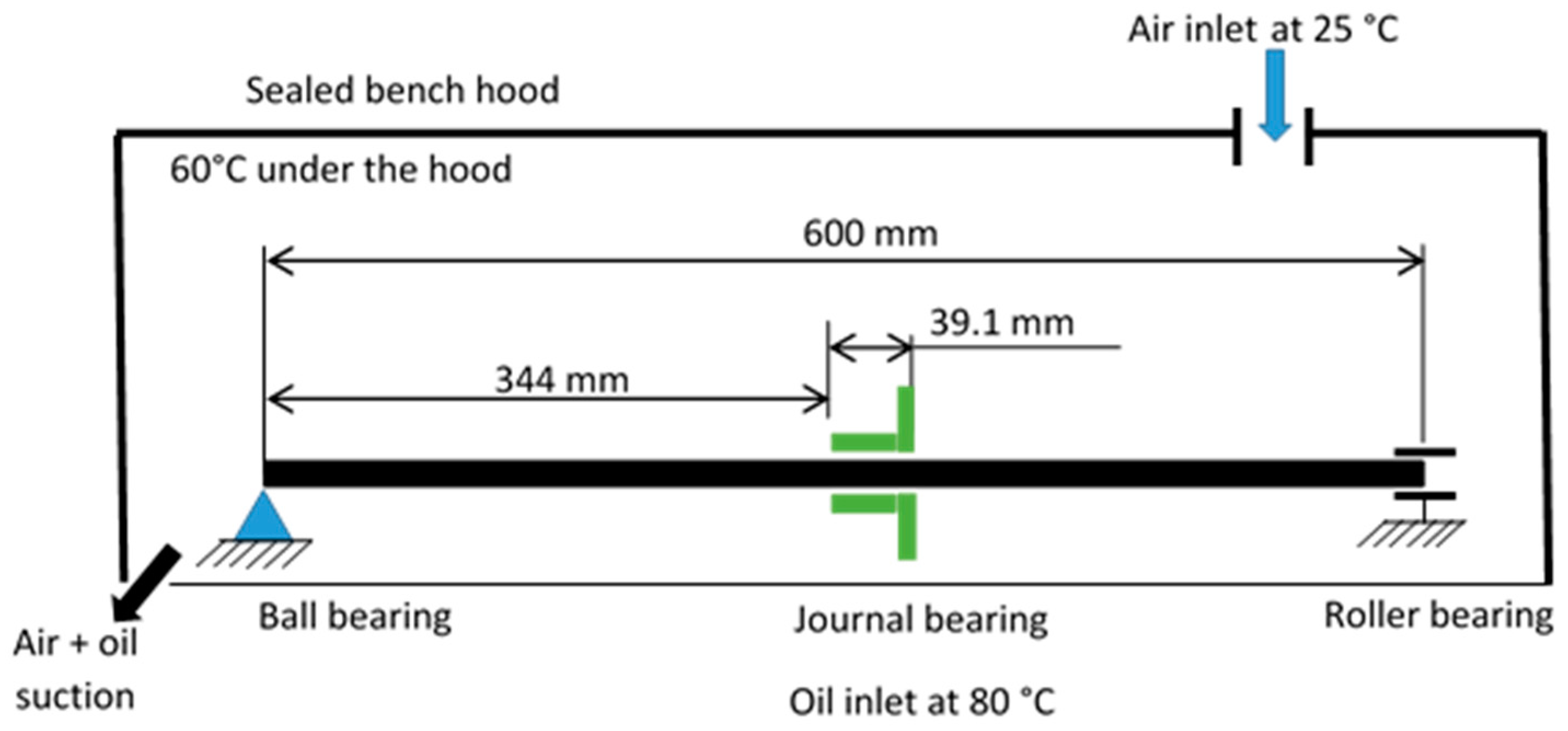
The hollow shaft is supported by roller bearings at its ends, while the journal bearing is mounted at 344 mm from the left-hand side end of the shaft, as seen on
Figure 2. The steel shaft is hollow, with an 8.5 mm thickness and 600 mm length (see
Table 2). The PTFE ring has a 4 mm thickness and an 80 mm length (see
Table 2). The loads applied on the shaft are equal to zero during start-up period, but the shaft was not in a perfectly centred position during the experiments (see
Table 1).
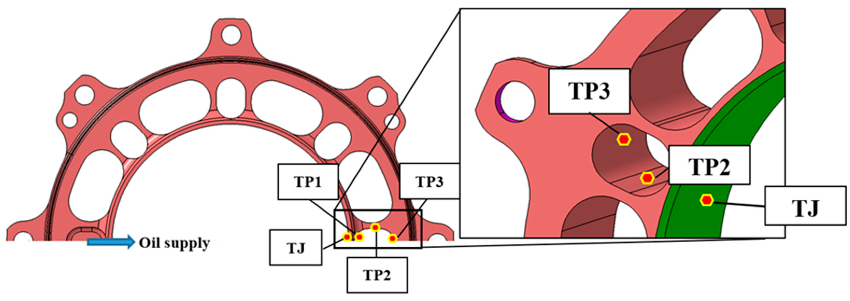
The temperature and pressure of the oil supply is measured during the tests. The temperature of the bushing is also monitored via 3 bimetal thermocouples, as well as the temperature of the PTFE ring (
Figure 3).
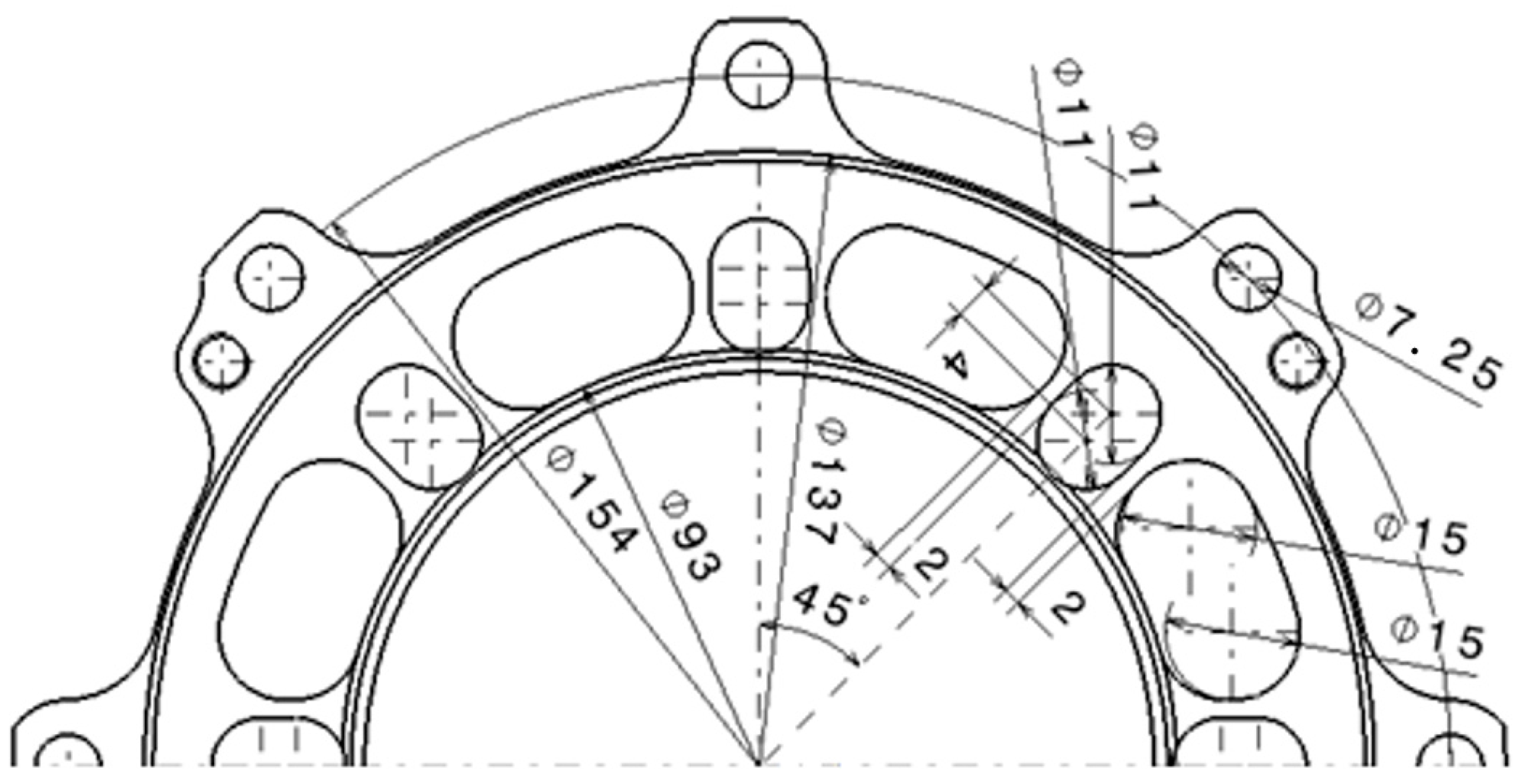
The bushing had a lightweight-design, its detailed geometry is presented on
Figure 4.
3. Experiment—Seizure during Start-Up Period of the Journal Bearing
Before start-up, the bench is heated for half an hour, with a constant oil and cool air flow until the thermal equilibrium is reached. Since the oil flow temperature is at 80 °C and the air flow has a constant temperature of 25 °C, the thermal equilibrium does not result in constant temperature in the solids. The temperature of the bushing is 70 °C under the PTFE ring (TJ) and 60 °C on the outer diameter (TP3). This is the reason behind the temperature difference measured by the thermocouples at the beginning of the experiment. The cool air flow is necessary to better represent the industrial application.
At start-up, a constant acceleration of 100 rpm/s is applied on the shaft, until 2000 rpm of rotational speed is reached. Later, a 50 s long stabilization phase starts, with constant rotational speed. Then, a second acceleration phase starts with 50 rpm/s acceleration rate. This procedure is presented in
Section 4.5.
The closure of the radial clearance can be observed through the decrease of the oil flow rate: at quasi-constant oil supply pressure, the oil flow rate decreases. At 120 s, the shaft and the PTFE ring come into contact, resulting in seizure.
The rapid non-uniform temperature change of the bushing could be observed through the sensors TP1, TP2, TP3 and TJ. The difference between TP1 and TP3 increase during the start-up period. This suggests that the heat generated by the journal bearing is not dissipated in the solids with sufficient speed, thus limiting the thermal expansion of the PTFE ring—while the shaft dilates freely. This is the reason for the closure of the radial clearance, the decrease of the oil flow rate and the seizure of the PTFE ring and the shaft.
4. Theoretical and Numerical Analysis
The computation tool of the present work was developed with special emphasis on cavitation, thus Elrod’s model was chosen to be integrated in it. Elrod’s equation is a conservative model both in the complete and oil film rupture zones. Generally, the journal bearing undergoes lubricant cavitation at high loads (due to the high eccentricity ratio) or at high rotational speeds (even at lower eccentricity ratios). High and uneven deformation fields might result in divergent zones in the oil film that cause cavitation at unforeseen locations. The present work’s test case (see
Figure 2 and
Table 2) undergoes cavitation due to the high rotational speed (at the end of the start-up period) and due to the complex geometry solid’s thermo-mechanical deformation.
The present journal bearing components’ unforeseen thermo-mechanical deformation is due to its uneven heat repartition in the complex geometry. This unpredictable behaviour results in such a deformed oil film that generate pressure fields which highly differ from the theoretical (undeformed) ones. An unpredictably deformed oil film might result in divergent (thus possibly cavitated) oil film at any point of the bearing, even at a low rotational speed. Elrod’s model is capable of taking into account the mass conservation in these ruptured zones, which makes it suitable for a wide range of applications, with high or unforeseen thermo-mechanical deformation.
The next section reveals in detail the hydrodynamic (HD) model used in this study. Then, the thermohydrodynamic (THD) model is presented with its numerical solution and discretization method. Further on, the heat equation in the fluid and in the solids is detailed, with the complete thermomechanical modelling. While coupling all of these models a steady-state thermoelastohydrodynamic (TEHD) model is obtained. Finally, taking into account the thermal inertia of the solids and neglecting the negligible transient terms in the fluid, the pseudo-transient TEHD model is obtained.
4.1. Elrod’s Model in the Isothermal (Hydrodynamic, HD) Regime
In 1974, Elrod and Adams [
12] presented an equation that is capable of taking into account the mass conservation in the cavitation region. Nowadays, this equation is called the Elrod’s model. Later, in 1981 Elrod and Adams developed an improved algorithm for their model [
13], which is applied in the present work.
Elrod’s model for the isothermal, HD case [
13]:
where:
| κ: | Filling factor | |
| t: | Time | (s) |
| β: | Bulk modulus of the lubricant | (1/Pa) |
| g: | Switch function | (-) |
| | In the active zone: g = 1,
In the inactive zone: g = 0 | |
| R: | Journal bearing radius | (m) |
| θ: | Circumferential coordinate | (rad) |
| z: | Axial coordinate | (m) |
| h: | Oil film thickness | (m) |
| μ0: | Dynamic viscosity of the lubricant | (Pa·s) |
| ρ: | Density of the lubricant | (kg/m3) |
| ρ0: | Reference density of the lubricant | (kg/m3) |
Compared to the Reynolds equation, it resolves the filling factor, which has a different definition the active and inactive (cavitated) zones:
In the active zone κ is the ratio between the density and the reference density: κ = ρ/ρ0,
In the inactive zone κ is the ratio between the non-cavitated lubricant volume and the total volume of the mesh element: κ = Vliquid/Vtotal.
Thus, a supplementary information is known in the cavitation region; the ratio of cavitated lubricant. This information defines whether or not pressure build up occurs in the convergent zones. Contrary to the Reynolds equation, which generates pressure in every convergent zone, without considering the oil mist properties. The pressure in both active and inactive zones of the journal bearing is calculated as:
where:
| p: | Pressure in the journal bearing | (Pa) |
| pcav: | Cavitation pressure of the oil | (Pa) |
In order to simplify the calculations, it is possible to rewrite the Elrod equation in a dimensionless form, with the dimensionless variables of Equation (19):
The transient term of the Elrod’s equation can be neglected due to the fixed position of the shaft (see
Table 1), which makes the temporal film thickness change a function dependent only on the thermal dilatation. The characteristic speed of thermal dilatation is the order of
C/
dt = 4.33 × 10
−7 m/s, where
dt is the full clearance closure time, (120 s in our case) and
C is the radial clearance (see
Table 1). The characteristic speed of the hydrodynamic pressure establishment can be estimated by the linear velocity of the shaft, in our case:
D/2 × ω = 2.09 m/s, for the rotational speed 5 s after start-up (where
D is the diameter of the shaft and ω is the rotational speed). This value strictly increases after start-up meaning that the hydrodynamic effects are least 2.09/4.33 × 10
−7 = 4.8 × 10
6 times faster than the thermal dilatation. This justifies our hypothesis to neglect the transient term of the Elrod’s equation.
4.2. Elrod’s Model in the Thermohydrodynamic (THD) Regime
In 1996, Vijayaraghavan published the dimensionless modified Elrod’s equation [
14], which is capable of taking into account the thermal phenomenon in the lubricant film:
Equation (4) is called the thermohydrodynamic (THD) Elrod’s equation, where the transient term was neglected for the same reasons as for the isothermal, HD Elrod’s model. The variables in Equation (4) are defined:
where the dimensionless variables are defined in Equations (16)–(21), and:
| y: | Radial coordinate in the film (m) |
| ξ: | Running coordinate in the radial direction (-) |
In order to determine the temperature field in the fluid, the heat equation should be written in the oil film (given by Dowson [
15] and Ferron [
16]). The heat equation in the fluid film is given in the following, dimensionless form with the dimensionless variables of Equations (16)–(21):
It is important to mention that the transient term in the heat equation is neglected due to its relatively small influence on the temperature field in the fluid. The transient term should be additioned to the left hand side of the heat equation. The dimensionless pseudo-transient term on the left hand side of the dimensionless heat equation is: (where the dimensionless time is: and the reference time equals to the length of the experiment: = 120 s).
This means that the transient term of the heat equation after 5 s (when the rotational speed is 500 rpm) is ω ×
t0 = (500/30 × π) × 120 = 6283 times smaller than the other terms of the dimensionless heat equation. Meaning that 5 s after the beginning of the test the transient term is negligible and due to the strictly increasing behaviour of the rotational speed of the shaft, it will stay negligible compared to the other (convective, diffusive and viscous) terms. It is also important to mention that right after start-up (between 0 and 5 s) the transient temperature change is the smallest due to the small heat generated in the fluid film, making it negligible on the whole time domain. Meanwhile the transient term of the heat equation in the solids cannot be neglected [
8,
9,
10,
11].
The three components of lubricant velocity in the film are (consecutively in the circumferential, radial and axial directions):
The definition of the Péclet number:
and the definition of the Brinkman number is:
where:
| Cp: | Heat capacity of the oil | (J/kg·K) |
| C: | Radial clearance | (m) |
| Kl: | Thermal conductivity of the oil | (W/m·K) |
| T0: | Reference temperature | (K) |
| μ0: | Reference dynamic viscosity of the oil | (Pa·s) |
The dimensionless speeds (consecutively in the circumferential, radial and axial direction) are defined as:
and the reference velocities are:
The dimensionless temperature is:
The dimensionless coordinates of equations are:
The dimensionless dynamic viscosity is:
The dimensionless pressure is:
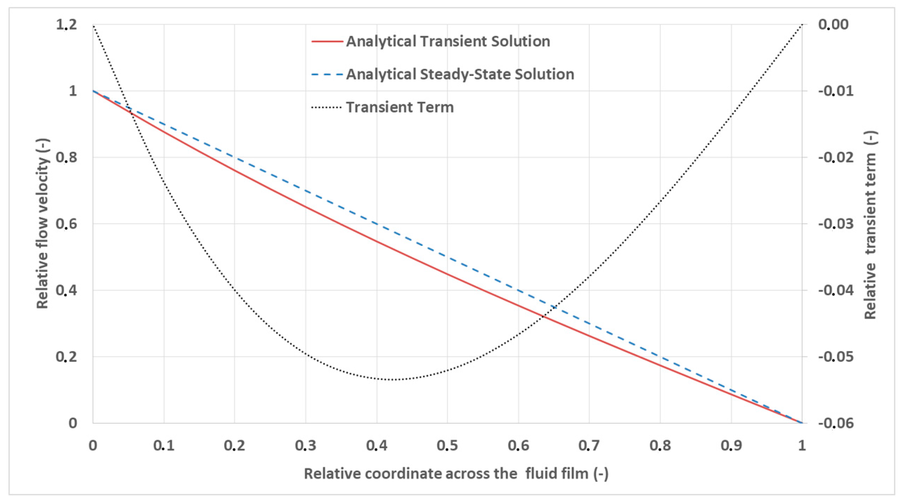
Since these equations are based on the linear momentum conservation equation, the transient term should be included in each direction. In our case, the acceleration of the shaft induces directly the transient term in the circumferential direction (which is a transient Couette flow), that influences the other (axial and radial) flow velocities. Thus, if the transient term in the circumferential direction can be neglected, the axial and radial flow velocities will not be influenced due to the shaft acceleration and the oil flow velocity can be determined through the above given steady-state equations.
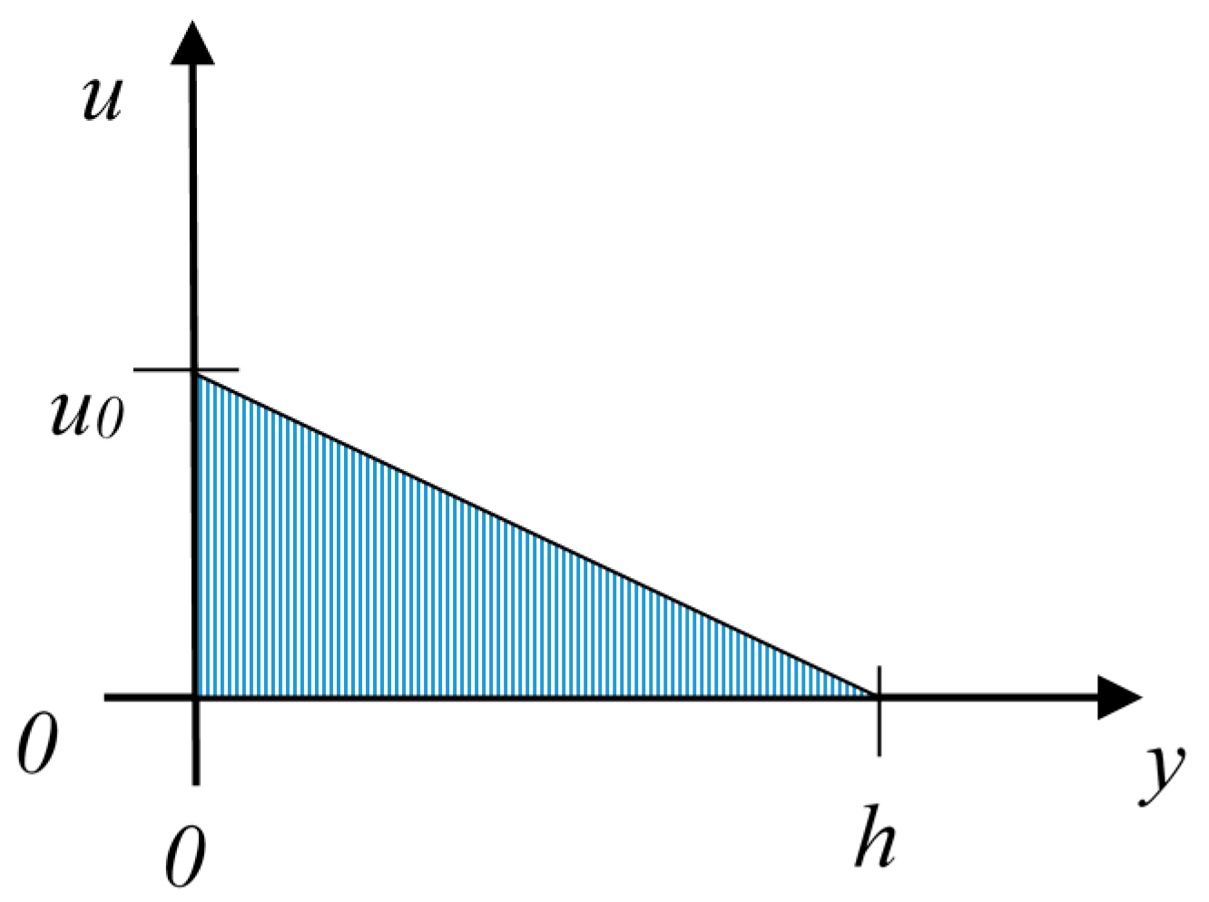
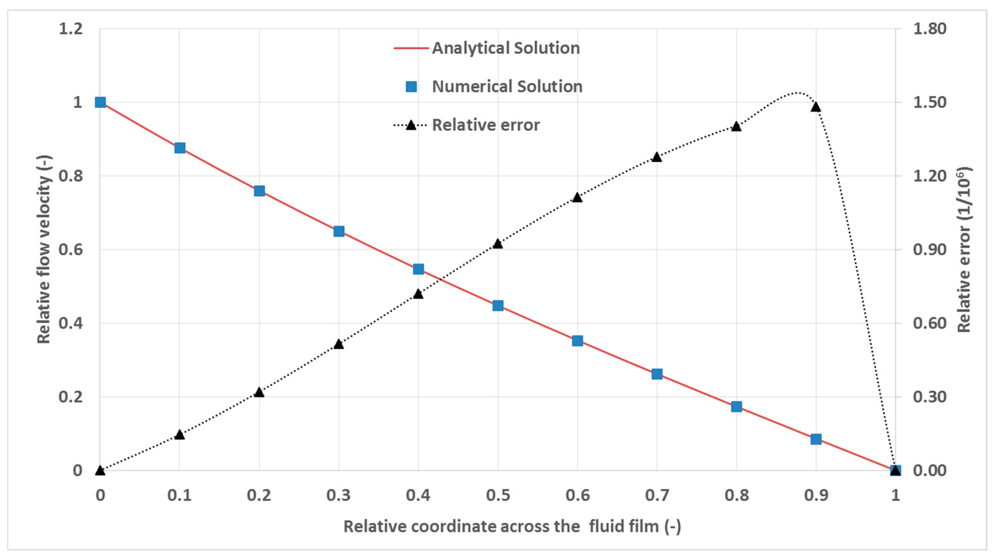
By decoupling the Poiseuille and Couette terms of the linear momentum equation, the velocity induced by the pressure field (Poiseuille flow) and the velocity induced by the surface movement (Couette flow) can be separated. Following the analysis described in
Appendix A, the maximal difference between the steady-state solution for each instance and the transient solution of the Couette flow for one constantly accelerating surface can be derived. As given in
Appendix A, Equation (A16), the maximal difference between the steady-state and transient solution can be obtained for the rapid (first) acceleration phase:
This value is constant during the acceleration phase (see
Appendix A), making it negligible for the whole time domain (since the linear velocity on the surface of the shaft after 5 s is ω × D/2 = 2.09 m/s).
4.3. Discretization Method for Elrod’s Model in the Thermohydrodynamic (THD) Regime
While the switch function (
g) defines the active and inactive zones, it also changes the equations describing the corresponding zones. The two zones require different modelling, since the equation is elliptic if
g = 1 and parabolic if
g = 0. The finite difference method differs for these two zones; thus, it is important to appropriately connect them: a robust and simple method was developed by Vijayaraghavan for the isothermal (HD) problem in 1990 [
17]. According to [
17] the first term of the left-hand side of the Equation (3) can be discretized as:
The second term of the left-hand side of the Equation (3) can be discretized as:
where the subscripts
i and
j correspond consecutively to the circumferential (θ) and axial (
z) direction of discretization. The subscripts +1/2 and −1/2 for an arbitrary
A variable, for both in the axial and circumferential direction are:
Vijayaraghavan’s algorithm can be adapted to the THD case (Equation (4)) in the circumferential direction as follows:
while in the axial direction the discretization has the following form:
Vijayaraghavan’s discretization method adapted for the last term of Equation (4) is:
The lubricant’s viscosity is determined by the equation of Walther-McCoull [
18]:
where:
| ν: | Kinematic viscosity of the lubricant | (cSt = m2/s × 106) |
| T: | Temperature of the lubricant | (K) |
| λ: | Dimensionless parameter | (-) |
| | (λ = 0.7 for the present ISO VG 32 oil) | |
| A,B: | Dimensionless parameters | (-) |
4.4. The Steady-State Thermoelsatohydrodynamic (TEHD) Simulation
After the THD computation, a thermomechanical computation was conducted with a commercial finite element software: the pressure field and the heat fluxes from the oil film were applied as mechanical and thermal loads on the corresponding surfaces of the PTFE ring and the shaft. The shaft and the bushing temperature fields are influenced by the temperature under the hood, equal to 60 °C during the experiment. This influence is introduced through a heat convection coefficient on every free surface (not being in contact with the oil) of the solids.
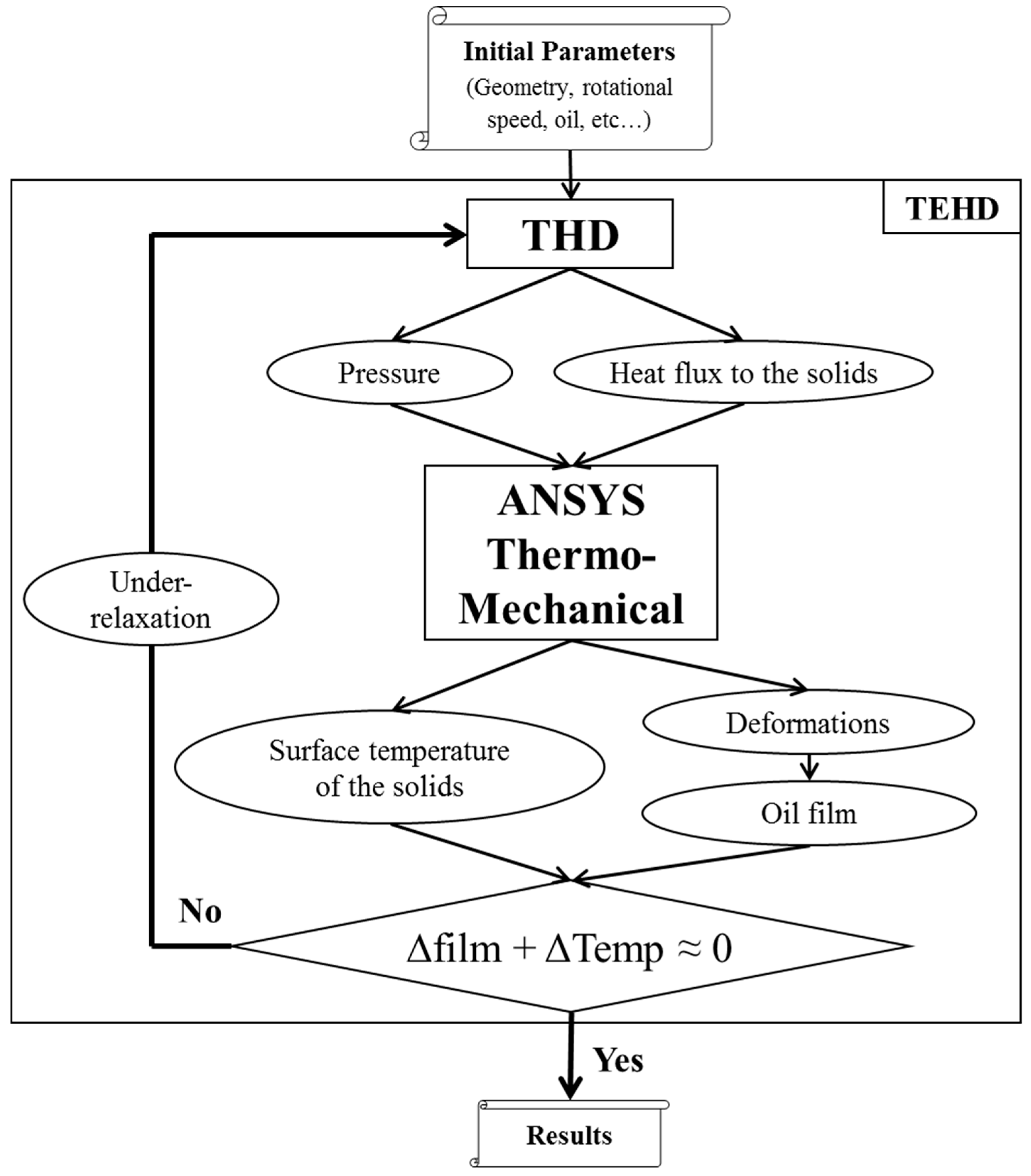
First, the commercial software determines the temperature field in the solids, then it resolves the thermal and mechanical deformation of the solids. The temperature field and the deformation of the nodes that are in contact with the oil are exported from the thermomechanical solver and after an under-relaxation are sent back to the THD solver, which is then re-executed (
Figure 5). The full convergence is reached when the deformed oil film and the temperature field of the oil film has converged for the same iteration. The relative convergence criteria on the pressure and temperature field was 0.01% for each node of the domain.
The heat equation in the solids (bushing, PTFE ring and the shaft) can be deduced from the first law of thermodynamics (without the convective, radiative and heat generation terms):
where:
| ρS: | Density of the solid | (kg/m3) |
| CpS: | Heat capacity of the solid | (J/kg·K) |
| k: | Thermal conductivity of the solid | (W/m·K) |
Since a no-slip condition is applied on the fluid-solid interface in terms of speed and temperature, the continuity of the heat fluxes at the solid-fluid interface can be expressed as:
The thermal boundary conditions on the surfaces of the solids which are in communication with the environment are represented with a heat flux induced by a heat convection coefficient (
h):
The thermal dilatation can be determined with the thermal dilatation coefficient for isotropic materials:
where:
| εth: | Thermal strain tensor | (-) |
| α: | Thermal dilatation coefficient | (1/K) |
In the solids, the linear elasticity equation for isotropic materials is applied:
where:
| u: | Displacement field | (m) |
| ü: | Displacement field’s second derivative with respect to time | (m/s2) |
| σ: | Stress tensor-field | (Pa) |
| F: | Volumetric forces | (N/m3) |
The Stress tensor-field can be determined with the following equation:
where:
| ε: | Strain tensor | (-) |
| C: | Fourth order stiffness tensor | (Pa) |
The stiffness tensor values can be obtained as follows:
where:
| E: | Young’s modulus | (Pa) |
| ν: | Poisson’s ratio | (-) |
| δ: | Kronecker delta | (-) |
The relative deformation field is the sum of the mechanical and thermal strain fields:
where:
| εm: | Mechanical strain tensor | (-) |
4.5. The Pseudo-Transient Thermoelastohydrodynamic (TEHD) Simulation
The above given method describes a steady-state TEHD analysis. A pseudo-transient TEHD analysis should also take into account the thermal inertia of the solids. The mechanical (or deformational) inertia of the oil and the mechanical inertia of the solids (shaft, PTFE ring and bushing) are usually neglected because the deformation of the solids is nearly instantaneous.
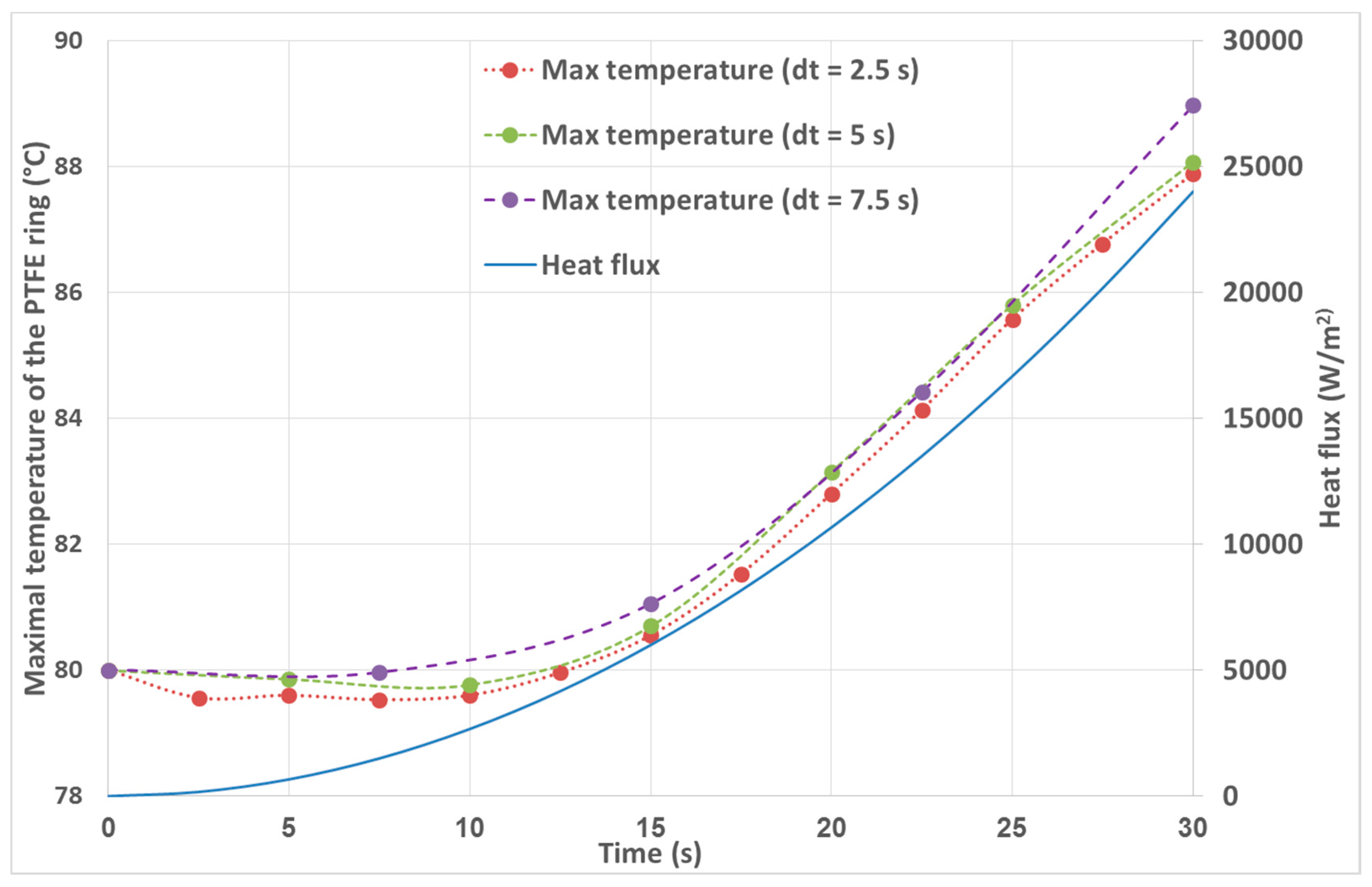
In order to correctly describe the thermal pseudo-transient behaviour of the solids, the time-step of the pseudo-transient simulation should be defined with great caution. A small time-step results in a high computation time, while a too long time-step might not describe precisely the case. Thus, a preliminary pseudo-transient thermal analysis was conducted on the 3D geometry of the test rig: a parabolic function of heat flux (representing the friction losses during acceleration multiplied by two) was established between 0 and 30 s. The initial state of this preliminary analysis equals to that of the real pseudo-transient analysis. At t = 30 s the heat flux on the surface of the shaft and the PTFE ring equals 24,000 W/m2.
Between 0 and 30 s after start-up, 3 different transient thermal analysis was executed with three different time-steps: 2.5, 5 and 7.5 s. For each type of simulation, the heat flux applied on the solids was the one at 50% of the current time step (i.e., for the step between 10 and 12.5 s the heat flux applied was the one at 11.25 s: 3375 W/m2).
The preliminary pseudo-transient TEHD analysis (
Figure 6) justifies that the ideal time-step for this geometry is 5 s. A shorter time step (2.5 s) gives results relatively close to the analysis with a 5 s interval, but the computational time is two times shorter. The longer interval (7.5 s) results in a different temperature field from the precedent two, thus the 5 s interval was chosen for the complete pseudo-transient analysis. The heat flux applied on the solids during the preliminary pseudo-transient thermal simulations was the double of the heat flux due to the losses in the oil film (obtained through THD calculations in the oil film at 2000 rpm with a radial clearance of 30 microns). The mean heat flux (friction losses multiplied by the rotational speed) of a journal bearing at such rotational speed and radial clearance was 12,000 W/m
2. At 5000 rpm, the mean heat flux is 22,000 W/m
2 for a journal bearing with radial clearance of 30 micron—meaning that the heat flux applied during the preliminary pseudo-transient TEHD simulation is always greater than that of the experiment. Due to the exaggerated thermal behaviour of the solids during the preliminary pseudo-transient analysis, this time-step ensures that it can describe well the real case during the pseudo-transient TEHD simulation at every given speed and time, from 0 to 120 s.
The test cycle was divided in 5 s intervals, resulting in 24 TEHD computation for the given start-up period (see
Section 4.5). For each interval, a TEHD analysis is executed. The first TEHD simulation is started after the heat-up period, when the PTFE ring has a temperature of 70 °C (TJ at 0 s), while the bushing temperature decreases gradually from 70 to 60 °C farther away from the PTFE ring.
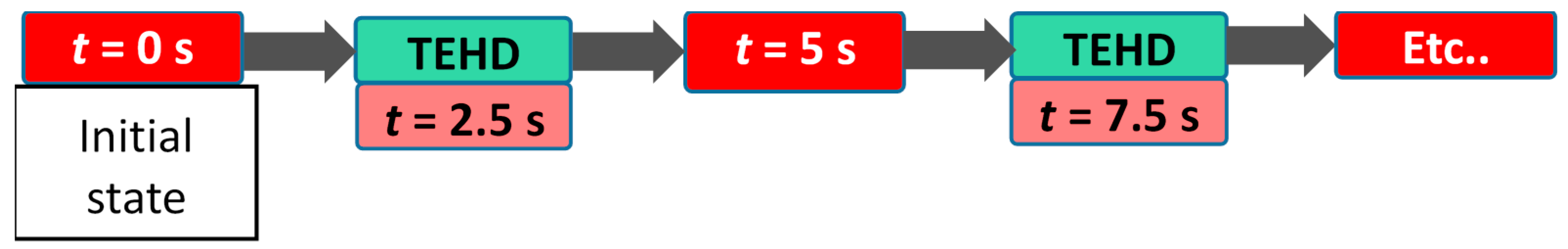
Although one pseudo-transient TEHD computation is run on an interval of 5 s, the convergence of the corresponding THD simulation in the oil film is executed on the mid-point of the transient thermal computation (
Figure 7). Thus, the heat fluxes obtained by the THD calculation in the oil film correspond to the mean heat flux coming from the oil film for any given time-step.
When the first TEHD simulation has converged, the initial temperature field is updated by the temperature field resulting from the precedent TEHD simulation (
Figure 7). The new initial temperature field (for the TEHD simulation starting from 5 s) is the one obtained from the beforehand converged simulation. The pseudo-transient simulation continues on like this for every 5 s long simulation, until the point of seizure is obtained.
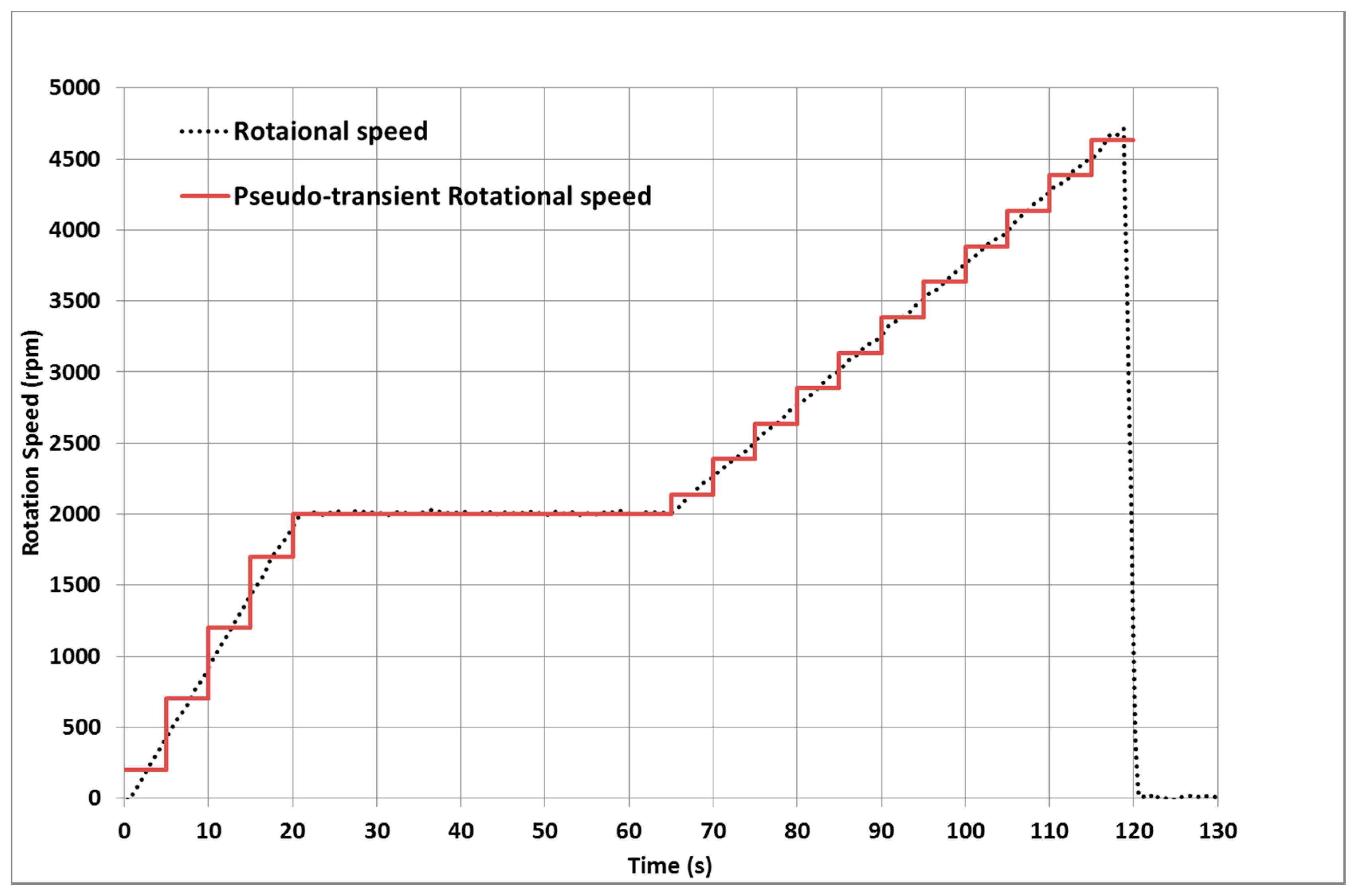
During the pseudo-transient simulation, the rotational speed of the shaft should be updated for each 5 s interval. The rotational speed taken into account for the thermomechanical and the THD computation is an averaged speed on the given 5 s interval (see
Figure 8). Since the rotational speed changes the fluid’s velocity under the bench hood, the coefficient of heat transfer between the oil mist and the free surfaces of the solids is also varied. This heat transfer coefficient is a linear function of the rotational speed.
The definition of the heat transfer coefficient was based on the article of Wodtke et al. [
19]. They found that the increasing rotational speed increases the heat exchange coefficient. Based on their results the heat transfer coefficients of the present study vary linearly between 250 and 4800 rpm. At 250 rpm, the heat exchange coefficient equals to 100 W/m
2·K and at 4800 rpm equals to 600 W/m
2·K.
In our case, the journal bearing had a fixed position, which was due to the geometry and assembly tolerances. The position of the bearing was measured at the beginning of the experiment (see
Table 1). The position was defined by the geometry of the test bench; thus, the transient term of the Elrod’s equation will be negligible against the Poiseuille and Couette terms (see
Section 4.1 and
Section 4.2).
5. Comparison to Cristea’s Test
In 2011, Cristea [
20,
21] published several experiments of a central groove journal bearing at equilibrium state. His test rig consisted of a rotating shaft of 80 mm diameter, with a 61 μm radial clearance at room temperature (22 °C). The length of the symmetric journal bearing had two 20 mm wide lands and a central, 13 mm wide central groove. The experiment was conducted at equilibrium position with constant speed and load. Cristea’s journal bearing had a steel shaft and a bronze bushing with an external diameter of 200 mm. The oil inlet temperature was constant, at 30 °C during the experiments of Cristea [
20] and 40 °C for [
21] (see
Table 3).
Temperature and pressure measurements were conducted at different axial and angular positions. The pressure was measured at every 10°, in 5 different axial sections (at 1, 4, 7, 12 and 17 mm from the end of the land). The temperature measurements were done at every 10°, at 5 different axial sections (at 1, 7, 13, 19 and 26.5 mm from the end of the land). Unlike in [
20], Cristea measured the oil flow rate and the resistant torque during his experiments in [
21].
The resemblance of Cristea’s test rig to our test bench is very high, thus a preliminary comparison of a steady-state TEHD simulation was conducted in order to compare the results at equilibrium state. The comparison of the steady-state TEHD analysis presented in this section is that of the experiment n°11 of [
21], where the applied load was 8000 N, at constant rotational speed of 4000 rpm, while the mechanical and thermal properties of the bushing and the shaft of the test bench of Cristea are presented in
Table 4.
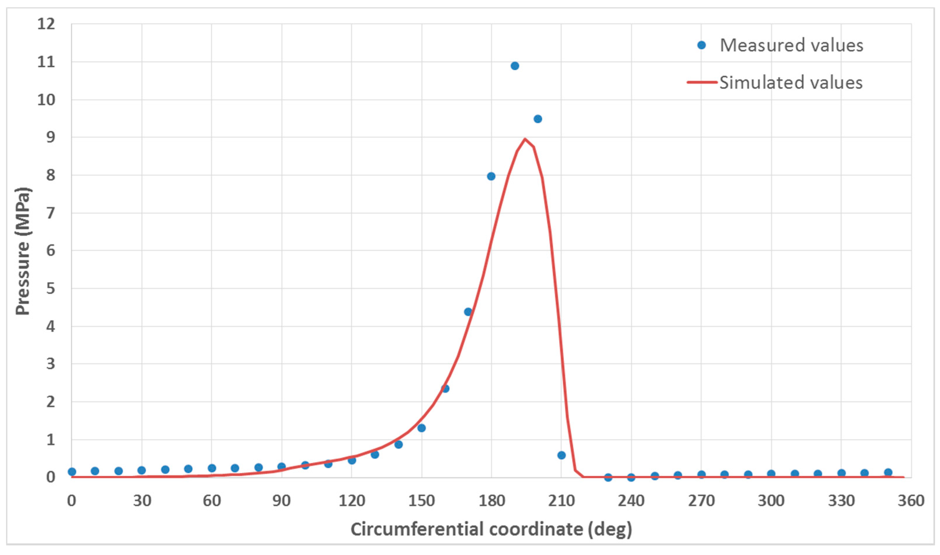
The measured and simulated pressures were compared in the plane 12 mm from the end of the journal bearing, the closest measurement plane to the mid-plane of the land. The pressure obtained from the TEHD simulation results are close to the measured values of [
21]—see
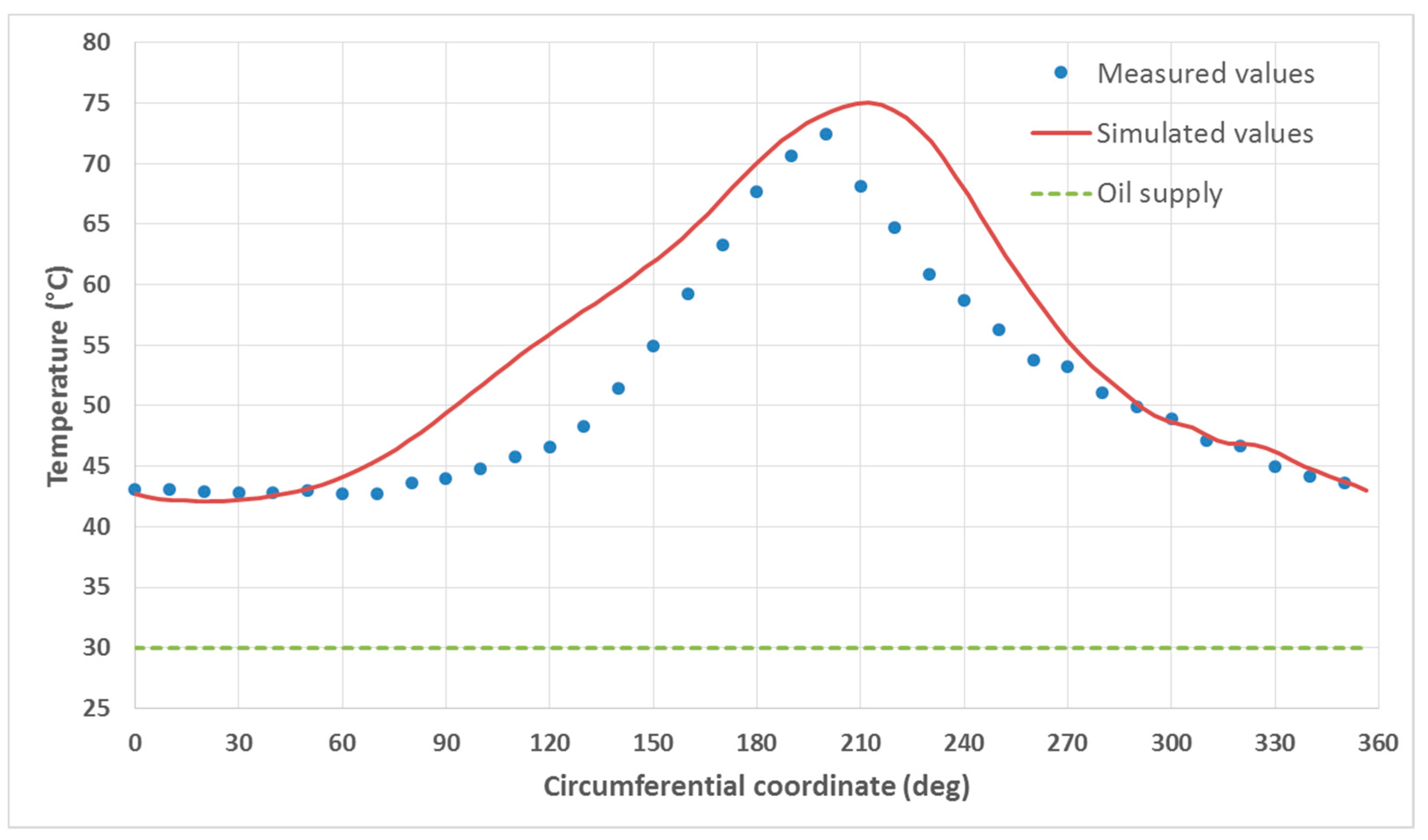
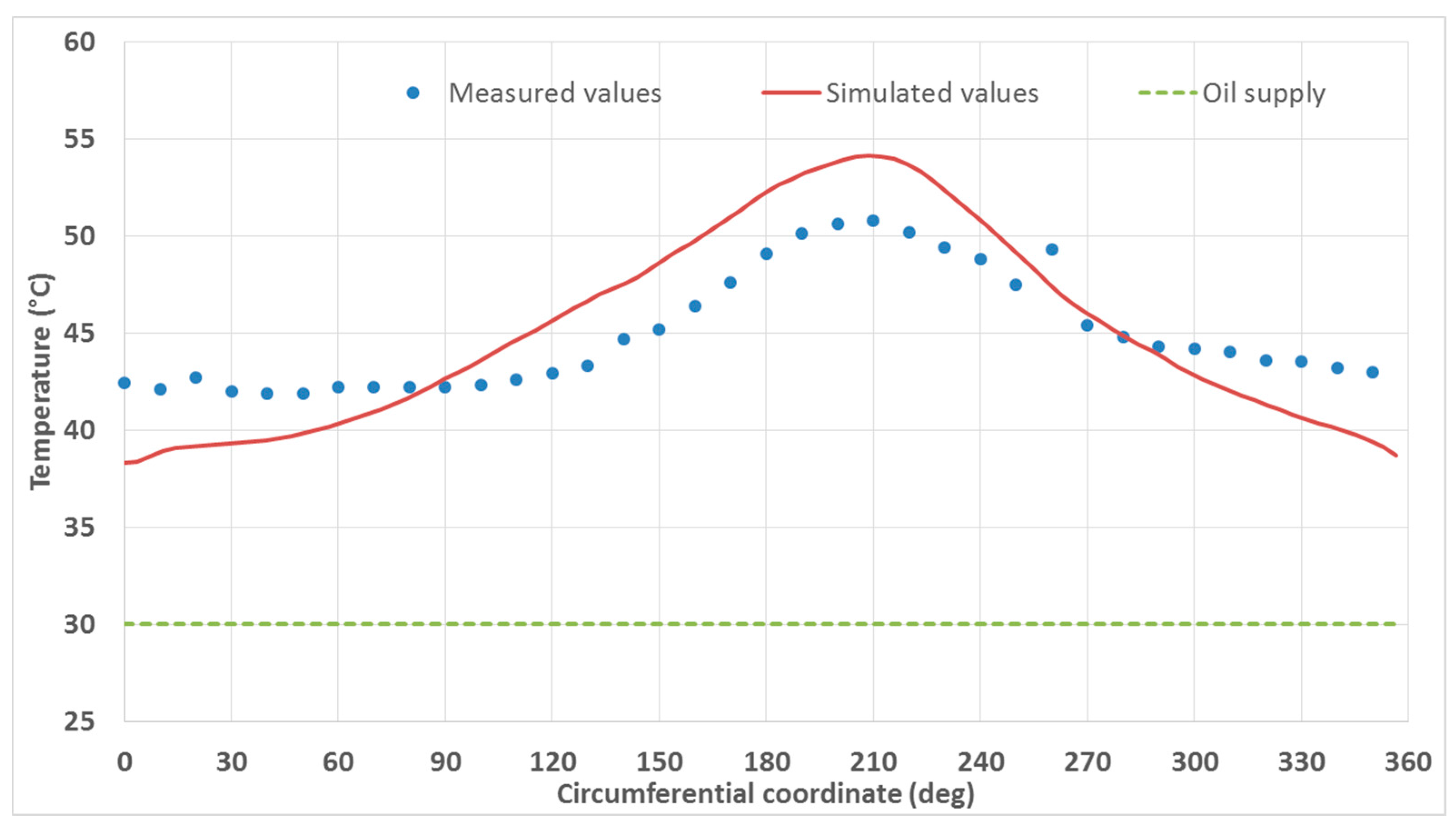
Figure 9. The simulated temperature field was also compared to the measured values, in the plane 13 mm from the end of the journal bearing (
Figure 10).
The difference in the pressure and temperature might be due to the high number of holes for the pressure and temperature sensors of the bushing. Yet another reason may be the lack of simulation methods in the groove: physically, the temperature field in the groove is dependent on the oil flow (speed and mass flow rate) in the groove and the pressure field is not constant in the groove [
20]. The present TEHD simulation tool is not capable of taking into account these phenomena: the pressure is supposed to be constant in the simulation tool and the oil temperature in the groove depends only on the temperature of the bushing and shaft temperature. The oil flow in the 4 mm deep groove cannot be taken into account with the Elrod (or Reynolds) equations. The difference in the simulated and measured temperature field is shown on
Figure 11.
Cristea also measured the oil flow rate and the resistant torque of the journal bearing. The comparison of the TEHD simulation and the experiment of these two values are presented in
Table 5. In spite of the difference in the pressure and temperature field, the simulated oil flow rate and resistant torque values are close to the measured ones.
6. Comparison to Present Results
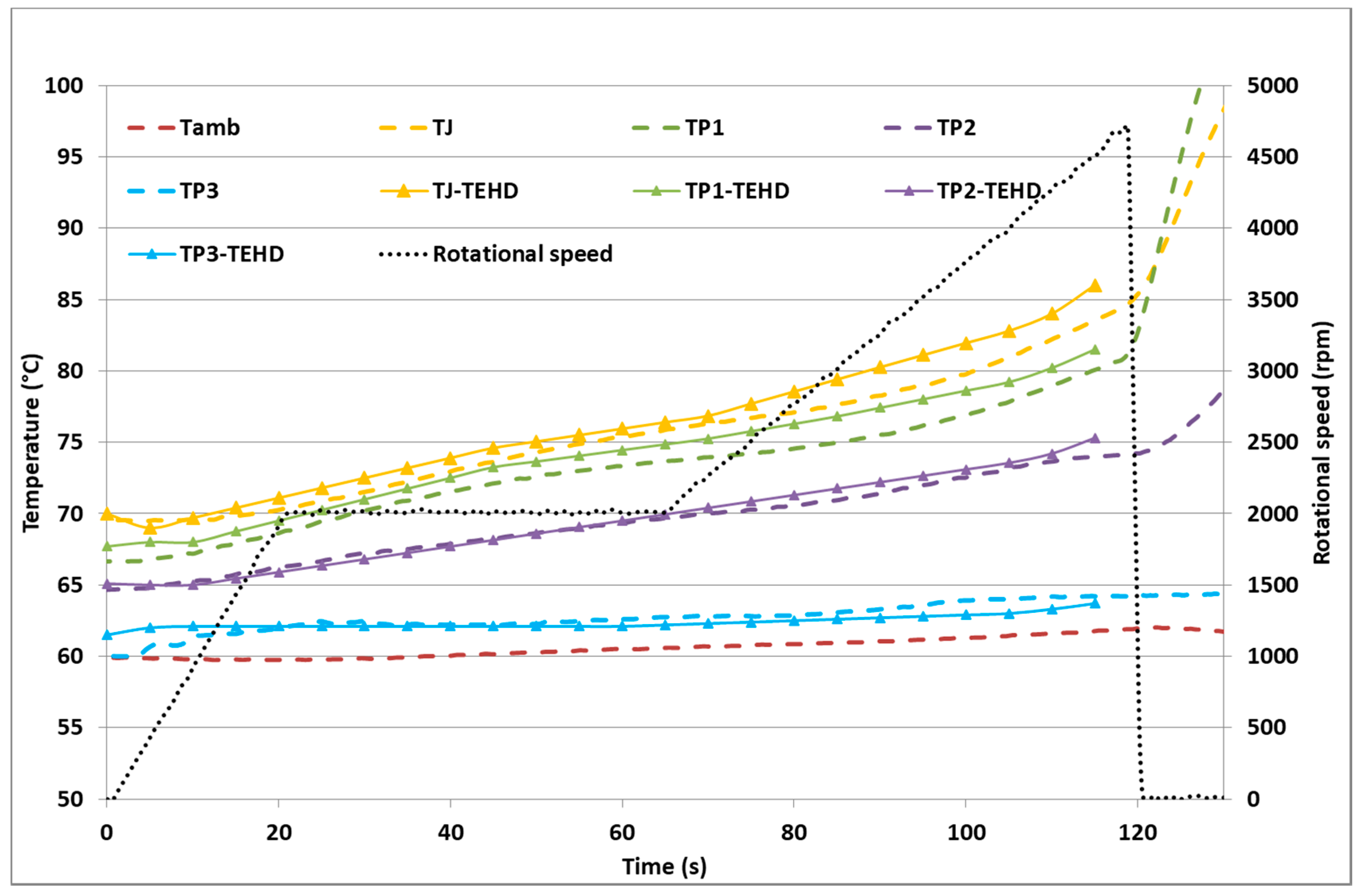
Further on, the comparison to this work’s test bench was executed. The comparison to the temperature measurements at different location of the bushing is presented on
Figure 12. Although the simulated temperature field is close to the measured one, there is still improvement to be done on the initial temperature field. The simulated temperatures at locations closer to the journal bearing (TJ and TP1) are in general higher, while the temperature at the furthest from the journal (TP3) are lower than the measured values. This indicates that the evolution of the heat transfer coefficient (h) should be non-linear, or a different linear slope, or a bi-linear law would be more suitable for the present application.
The differences in the temperature gradients at the measured points underline the fact that the PTFE ring and the lightweight geometry of the bushing function as an insulator. At 80 s, the temperature of TJ increased by 14 °C, TP1 by 12 °C, TP2 by 5 °C and TP3 by 2.5 °C. Since the bushing was fixed on its outer rim (where the temperature increment is close to 0), the thermal dilatation is limited in the outer direction, while the hollow steel shaft can freely dilate and decrease the clearance. The PTFE ring’s higher temperature and lower Young’s modulus limit the PTFE’s ring’s options to dilate outwards, towards the steel bushing. This means that the PTFE ring partially dilates towards the interior, which accelerates even more the clearance closure.
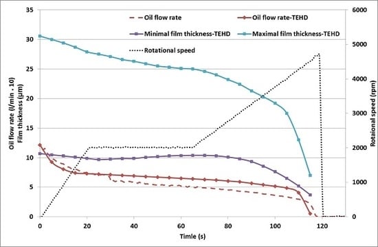
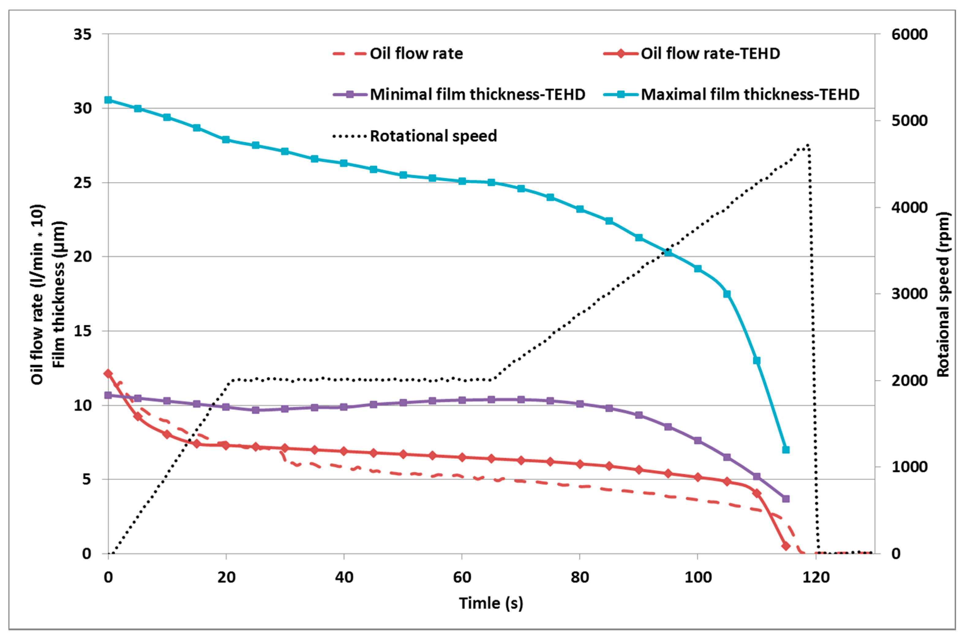
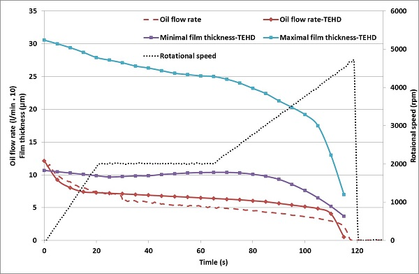
By comparing the TEHD-simulated oil flow rate to the measured one, the present method’s capability to describe the behaviour of the central groove journal bearing (see
Figure 13) is justified. The evolution of the minimal and maximal film thickness reveal (
Figure 13) that the journal bearing was close to reach its equilibrium state at the end of the stabilization phase (at 70 s): the minimal film thickness was already in the increasing phase, while the maximal film thickness was stabilizing. This stabilization can be observed on the temperature field also: the temperature increases of the TJ and TP1 sensors were slowing down (see
Figure 12).
After the beginning of the second acceleration phase, the minimal and maximum film thickness decrease and the gradient of the temperatures TJ and TP1 continue to increase. The brutal part of the seizure commences 10 s before the complete seizure, at 105 s. After this time, the film thickness exponentially decreases, limiting the oil flow rate, thus rapidly increasing the shear losses.
At 115 s, the simulated temperature field of the PTFE ring jumped to 160 °C, which is close to the temperature limit of the material. The TEHD simulation at 120 s did not converge due to divergence in the THD computation in the oil film: the temperature difference between the two solids and the oil supply was too high for the given mesh (see
Section 7) and for the given oil film thickness.
At
t = 0 s, the sum of the maximal and the minimal film thickness is 44 microns, which means that the initial diametral clearance at 22 °C (2 ×
C = 104 μm, see
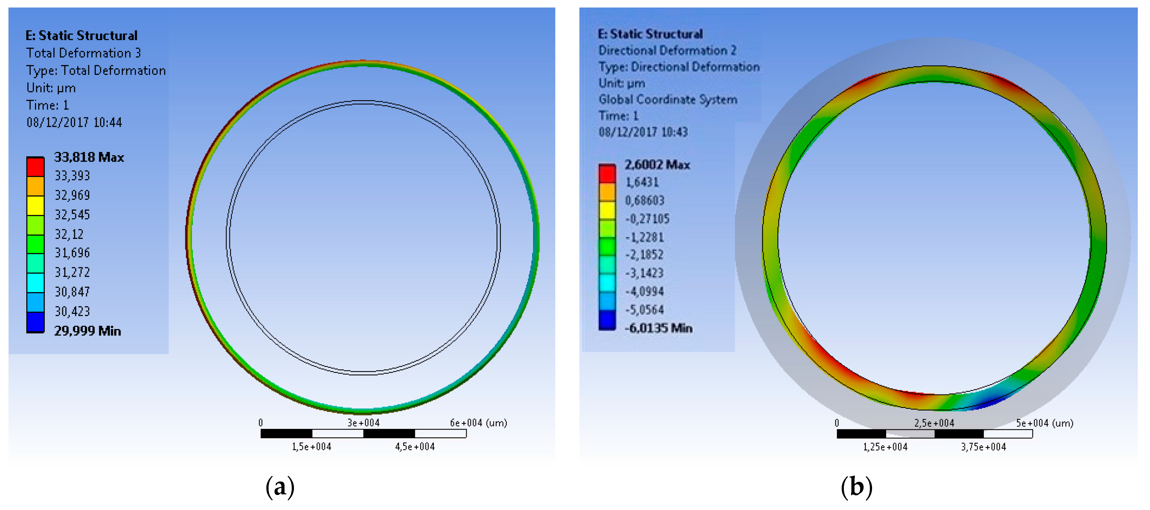
Table 1) was decreased during the heating up of the bench. In order to justify this, the deformation after the end of heat-up sequence should be examined, at perfectly centred position of the shaft. The shaft and ring deformations of this analysis are presented on
Figure 14.
On the left side of
Figure 14, the deformation of the outer surface of the shaft is revealed: the mean deformation in the radial direction is 31.9 microns outwards (the two concentric black circles represent the undeformed shape of the shaft). On the right side of
Figure 14, the deformation of the PTFE ring demonstrates that the ring expands by 1–2 microns. This means that the diametral clearance closes by 2 × 31.9 microns due to the shaft dilatation, resulting in a 40 micron diametral clearance, which is then slightly opened up by the 1–2 microns expansion of the ring, which is close to the sum of the maximal and minimal film thickness that is displayed on
Figure 13.
7. Computational Effort
The present method consists of two separate, yet connected models. The first one is the THD Elrod’s model describing the oil film between the solids. The mesh of the regular, cylindrical domain of the oil film had a uniform mesh size with 100 uniform divisions in the circumferential direction and 50 uniform divisions in the axial direction. Across the fluid film, in the radial direction the domain was divided into 25 equal parts.
The shaft also had a uniform, hexahedral mesh, with four elements in the radial direction, 200 elements in the axial direction and 100 elements in the circumferential direction. The bushing and the PTFE ring had a non-uniform tetrahedral mesh, with a maximum size of 1 mm, with local refinements. The overall number of elements for the finite element model in ANSYS Thermal-Mechanical was 500,000 (100,000 elements for the cylindrical shaft and 400,000 elements for the bushing and the PTFE ring) with 300,000 nodes.
Across the “thin” parts of the bushing, the solid was divided into at least three elements. The PTFE ring had 4 (gradually increasing sized) elements across its 4 mm thickness. These criteria ensure the correct modelling of the temperature gradient across the thin thicknesses. The mesh for each solid was a linear mesh, meaning that the nodes of the elements were situated only in the corner points of the elements, without any nodes on the edges or on the faces of the elements. A mesh dependency analyses was conducted for the most important parameters of the FEM model, which is not detailed in the present work.
One thermomechanical computation took around 4 min on a medium-performance computer, with four processors (each 1.5 GHz). One THD computation takes around 7–8 s with two medium-performance processors (each 1.5 GHz). The criteria of convergence for the TEHD computation was 0.1% of relative error on the fluid film and 1% relative error of temperature on the fluid-solid interfaces.
The length of each TEHD analyses depends on the rotational acceleration of the shaft, the rotational speed of the shaft and the temperature gradient. This problem gave a highly varying computation time for each TEHD simulation. The first computation (from t = 0 s to 5 s) was 5 h long, while the computational effort for the rest varied between 30 min and 1 h. The total computational time for the 24 TEHD computations was 22 h, which is a reasonable computational cost for such an industrial application.
8. Conclusions
The experiments determined that the current structure of the journal bearing can cause seizure during start-up period. The experiment with temperature measurements demonstrated that the PTFE ring temperature increases with a higher rate than the temperature of the bushing and the shaft. This constrains the thermal expansion of the PTFE ring, while the dilatation of the steel shaft is unperturbed. Since the PTFE ring’s Young’s modulus is nearly two times smaller than that of the steel bushing, the hotter the PTFE ring is, it dilates more towards the interior (and slightly outwards, towards the steel the bushing), accelerating the clearance closure.
The clearance closure was also observed through the decrease of the oil flow rate. As the clearance closes, the same oil supply pressure results in a smaller oil flow rate; resulting in a higher oil temperature in the journal bearing. This phenomenon also accelerates heat-up of the solids, thus the clearance closure. These are the reasons leading to seizure at start-up. Moreover, with a longer stabilization phase and slower acceleration rates a stable operation could be possible to achieve.
A pseudo-transient TEHD model was developed and validated to the experiment. The validation proved that the TEHD Elrod’s model is capable of correctly describing the behaviour of the journal bearing. The simulation proved our theory that the bushing’s temperature increase is limited due to the low heat conductivity coefficient of the PTFE ring and the fast start-up sequence. Furthermore, the PTFE ring under the lightweight bushing is not recommended for such a rapid start-up sequence.

 ,
, 


