Comparison of Perturbed Reynolds Equation and CFD Models for the Prediction of Dynamic Coefficients of Sliding Bearings

Department of Mechanical Engineering, The University of Akron, Akron, OH 44325-3903, USA
*
Author to whom correspondence should be addressed.
Lubricants 2018, 6(1), 5; https://doi.org/10.3390/lubricants6010005
Submission received: 10 November 2017
/
Revised: 10 December 2017
/
Accepted: 6 January 2018
/
Published: 10 January 2018
(This article belongs to the Special Issue Friction and Lubrication of Sliding Bearings)
Abstract
:The accuracy and utility of rotordynamic models for machinery systems are greatly affected by the accuracy of the constituent dynamic bearing models. Primarily, the dynamic behavior of bearings is modeled as linear combination of mass, damping, and stiffness coefficients that are predicted from a perturbed Reynolds equation. In the present paper, an alternative method using Computational Fluid Dynamics (CFD) with a moving boundary is used to predict the dynamic coefficients of slider bearings and the results are compared with the more commonly employed perturbed Reynolds equation model. A linear slider bearing geometry is investigated and the results serve as precursors to similar investigations involving the more complex journal bearing geometries. Time and frequency domain methods for the estimation of dynamic coefficients are shown to give comparable results. For CFD with a moving boundary, temporal inertia is found to have a significant effect for a reduced, squeeze Reynolds number less than one. The temporal inertia effect is captured through an added mass coefficient within the dynamic model of the bearing.
1. Introduction
The thrust of this paper is to introduce an alternative method for the prediction of the dynamic coefficients of bearings through the use of transient Reynolds equation and transient Computational Fluid Dynamics (CFD) with a moving boundary in lieu of the more commonly applied perturbed Reynolds equation. The proposed method is analogous to experimental methods of Tiwari et al. [1] used to determine the dynamic coefficients wherein a sinusoidal perturbation (input) is correlated with the corresponding transient force (output) of the bearing. The results obtained with this method are compared first for a self-acting linear slider bearing and pure squeeze motion between parallel plates. As both CFD (with inertia) and Reynolds equations (without inertia) are employed in the present work, the literature review will first cover previous work examining inertia effects in bearings, while, in the present work, Reynolds numbers are kept low and consequently inertia effects minimized, the role of inertia warrants discussion at this stage as subsequent applications will involve marine bearings. Marine bearings typically employ lower viscosity water as the lubricating fluid that will increase Reynolds numbers and consequently inertia may play a significant role in the static and dynamic behavior of bearings. Subsequent to inertia effects, work examining methods of calculation of the dynamic coefficients is reviewed.
The approach of characterizing the dynamic properties of bearings using CFD is rather of recent times owing to the widespread availability of increased computational power. CFD anchored methods allow accounting for both inertia and 3D effects as well as accommodation of complicated geometries. Under the standard Reynolds equation perturbed solution or transient Reynolds equation solution, inertia and three-dimensional effects are assumed to be negligible and excluded. Snyder [2] in 1963 recognized that the fundamental theory of hydrodynamic lubrication discounts the inertia effects and decided to investigate the effect of the advective inertia terms, which are nonlinear terms of the form, , in the performance of the slider bearing. His interest was motivated by the increasing operational speeds of bearings in combination with the low viscosities offered by either gases or liquid metals; the latter were becoming lubricating fluids of great interest in the context of the Magneto-HydroDynamic (MHD) bearing technology. Generally, he noted correctly, that the combination of high speeds and low viscosities generate higher Reynolds numbers that may require the consideration of the inertia effects. In this context, he mentioned earlier work done by Osterle, Hughes and Saibel, which in separate papers [3,4,5] considered the effects of higher Reynolds numbers characterizing high speed lubrication. Snyder noted that the technique used by the Osterle group approximated the inertia terms by an average value across the lubricating film, allowing the equations of motion to be integrated across the film in order to obtain pressures, their gradients and corresponding mass flow rates. The author’s [2] consideration of the nonlinear inertia terms of the reduced Navier–Stokes equations (NSE) accounted for the local variation of the inertia terms across the film as well as in the direction of the slider motion. His method involved the definition of a stream function and its expression through a series solution.
Osterle and Hughes [3,4] studied journal and thrust bearings, using both liquid and gases as working fluids. Starting from Navier–Stokes equations (NSE) in a simplified form (e.g., , where for a hydrostatic thrust bearing), they isolated the inertia terms and through parametric studies determined the effect of inertia on both flow and steady load carrying capacity. In effect, they worked within the framework of the NSE without recourse to the Reynolds equation. They found that the load carrying capacity decreases drastically with the increase of the inertia parameter, (which drives the radial pressure gradient ), and thus concluded that at high rotational speeds fluid advective inertia must be included in calculations.
Launder and Leschziner [6] in 1978 presented an integro-differential method for calculation of laminar flow considering inertia in finite-width bearing self-acting bearings. They used the numerical advances involving finite volume equation discretization introduced by Patankar and Spalding [7] to fully account for inertia effects, cast the equation in the form of primitive variables, and implemented new marching techniques to simulate flow and pressures in finite width self-acting slider bearings. To quantify the inertia effects due to changes in the slider (or fluid) velocity, they used a reduced Reynolds number based on the average film thickness (). Ultimately, they concluded that inertia is an important factor in the design of slider bearings with steps or pockets (hydrostatic) when optimal pressure and flow (leakage) prediction are desired.
Chen and Hahn [8] demonstrated in 1998 the advantages of using CFD software in modeling plane and stepped sliders, and journal bearings. CFD allowed the study of the contribution of the inertia terms to pressure and flow pattern prediction when compared with results yielded by the Reynolds equation. Reduced Reynolds numbers () for the slider bearing and () the journal bearing, respectively) between and were evaluated. For the long slider and step bearings, it appears that the effect of inertia terms introduced by the CFD is not considerable when compared with the Reynolds equation results; however, for the journal bearing, the difference in these results (CFD vs. Reynolds) seem to be noteworthy.
Dobrica and Fillon [9] applied both CFD and Reynolds equation in the analysis of Rayleigh step bearings. The authors summarized advantages and disadvantages of both techniques. The authors found that the Reynolds equation provides sufficiently accurate results for thin films (<200 m) despite an inability to capture advective inertia effects localized at the bearing step. For thicker films (up to 500 m), CFD is necessary to accurately capture advective inertia effects, which result in appreciable differences in CFD and Reynolds equation results.
Vakilian et al. [10] also analyzed the Rayleigh step bearing using CFD in a manner similar to Dobrica and Fillon [9]. Vakilian et al. isolated advective inertia effects by numerical solving the two-dimensional linear momentum equations both with and without the advective inertia terms. The authors found that the assumption of no advective inertia leads to local errors in the computation of pressure upstream (under-prediction) and downstream (over-prediction) of the bearing step. While the assumption of no advective inertia leads to localized errors in pressure, it also leads to under-prediction of temperatures throughout the whole bearing.
CFD has also been used extensively in the simulation of bearings with pockets and surface texturing. Fouflias et al. [11] applied the commerical CFD code ANSYS CFX in the analysis of thrust bearing designs with both pockets and suface texturing (dimples). The authors compared steady-loads predicted by CFD for different thrust bearing designs.
As described above, seminal work has been performed to determine the effects of advective fluid inertia on steady flow, pressure, and loads generated by both slider and journal bearings. These efforts also focused on improving the computational tools available to the lubrication engineering community to predict bearing properties under steady conditions.
More recently, attention has been paid in complementing the previously mentioned work with information characterizing the dynamic performance of bearings, specifically through the prediction of linearized dynamic coefficients of various self-acting bearing systems.
Zeng et al. [12] recognized that the dynamic characteristics of an air slider bearing are important in determining the performance and stability of a hard disk drive, and used modal analysis to identify these dynamic characteristics. They instituted a procedure for evaluating both the modal parameters and stiffness and damping matrices by using a combination of the slider suspension equations and the generalized Reynolds equation. The slider was then subject to small disturbances that were a function of time. In this paper, the frequency response function (FRF) is first calculated from the excitation and response; then, the modal parameters are estimated from the FRF, and the stiffness and damping matrices are then derived from these parameters. The authors also determined that the squeeze term in the Reynolds equation affects rather substantially the slider stiffness. They warn with regard to the differences in the stiffness value obtained from steady state Reynolds versus the transient Reynolds.
Lin and Hung [13] studied slider bearings with exponential and linear film profiles, and took into consideration the bearing squeeze action. They applied small amplitude oscillations about the steady state position in order to obtain a perturbed form of the Reynolds equation. They introduced perturbations into the dimensionless pressure and dimensionless film thickness, and respectively. By introducing these expressions in a dimensionless, transient form of the Reynolds equation for infinitely long slider bearings, they obtained two differential equations governing the evolution of the static, , and dynamic, , pressures. The stiffness and damping coefficients of the bearing were determined by integrating the dynamic pressure. The steady load as well as the stiffness and damping coefficients of slider bearings with linear and exponential film profiles are compared over a range of inlet–outlet film thickness ratios (taper ratio).
Lin et al. [14] using a similar analytical technique to the one described in [13], analyzed the steady-state and dynamic performance characteristics of the same bearing as in [13], but this time applied to a Newtonian couple stress fluid as the working fluid. When the performance of the exponential film slider was compared to that of the linear slider, the authors found that the exponential film slider operated at smaller flow rates, and exhibited better dynamic and stiffness coefficients, given the same taper ratio.
Lin et al. [15] also studied the linear slider bearing behavior when it is lubricated with an electrically conducting fluid and subject to a transverse magnetic field. A body force introduced in the Reynolds equation for the infinitely long slider takes into account a uniform transverse magnetic field B, which creates a Lorentz type force. The result is a Reynolds equation applicable to MHD fluids. The nonlinear dynamic stiffness and damping coefficients are obtained by evaluating the partial derivative of the MHD induced film force with respect to the minimum film thickness and with respect to the squeeze velocity, respectively.
Naduvinamani and Marali [16] analyzed the dynamic characteristic of a plane inclined slider bearing using a micropolar fluid. They started with the NSE modified to account for the micropolar fluid and derived a modified Reynolds equation for the micropolar fluid. Then, in a manner similar to Lin et al. [13], perturbations were introduced into the film thickness and pressure to derive a perturbed set of Reynolds equations. The stiffness and damping coefficients were respectively obtained from the real and imaginary components of the integrated dynamic pressure, i.e., the dynamic or perturbed component of the bearing load.
Hanumagowda et al. [17] studied the characteristics of a land tapered slider bearing using an MHD electrically conducting, couplestress active fluid. The fluid was subject to a uniform magneti field. Just like Lin et al. [15], the performance was tied to the variation of the Hartman number and a couplestress parameter. The reduced (no advective inertia terms) NSE were modified to account for the couplestress fluid, and the body forces due to the magnetic field were introduced. Using the continuity equation integrated across the film, a 1D modified Reynolds equation accounting for the MHD and couplestress fluid and containing the squeeze term was generated. The stiffness coefficient was obtained by differentiating the force, obtained from the pressure integration, with respect to the minimum film thickness. The dynamic damping coefficient was similarly obtained by differentiating the same force with respect to the squeeze velocity.
2. Scope of Work
The Introduction section gives an image of the methods used in the investigation of the performance of slider bearings in terms of pressure, load, and methods for obtaining the dynamic coefficients. Most generally, the methodology, whether for the self-acting slider or journal bearings, is to obtain a set of steady and perturbed Reynolds equations and calculate the stiffness and damping coefficients by integrating the resultant dependent variable fields, which satisfy those equations. In this context, one has to mention also the landmark papers of Lund [18,19], which is at the basis of the majority of the perturbed Reynolds equation methods applied in determining the linearized stiffness and damping coefficients. Usage of CFD with NSE or Stokes equations has been rare in the context of bearing lubrication, and mostly applied to determining the impact of advective inertia on steady-state load.
In this paper, we will introduce a method whereby the dynamic coefficients are calculated from the transient forces that develop in the bearing which is subjected to small, harmonic oscillations of the domain boundary. The method can be applied to bearings in which transient forces arise from solution of the transient Reynolds equation or transient CFD. For matters of emphasizing the proposed methodology, we are applying it here to the simple, infinitely long, linear slider bearing and pure squeeze motion between parallel plates (infinitely long). Comparisons are made between the dynamic coefficients predicted by the perturbed Reynolds equation and the alternative method in which both the transient Reynolds equation and transient NSE serve, separately, as the governing equations. Where possible, comparisons are also made between the proposed method and analytic solutions. The method can readily extended to the analysis of more complex bearing geometries and serves as the basis for subsequent investigations to determine the dynamic coefficients of marine bearings. The effects of temporal inertia and as a consequence, added mass coefficients, are also discussed.
3. Geometry
Figure 1 depicts the infinitely long (length L in the z-direction is infinite), linear slider bearing geometry. The geometric and operational parameter values of the bearing are motivated by those associated with rubber-lined, marine bearings where individual staves create a local geometry similar to that of a series of infinitely long slider bearings assembled in the circumferential direction. The lubricant considered is water with a kinematic viscosity of (m2 s). The minimum film thickness of the linear slider bearing is (mm), which is based on the radial clearance of an actual marine journal bearing with a diameter of (mm). For a traditional hydrodynamic journal bearing, the ratio of the radial clearance and the bearing radius, , is generally between 1/500 and 1/1000. For marine bearings, is slightly larger (3.4/500) [20]. The nominal bearing width (mm) satisfies motivated by marine bearing dimensions.
The sliding velocity (m s) results in a sliding Reynolds number () in which the bearing flow can be considered laminar as turbulence is considered to occur at a Reynolds number of approximately 2000 [21,22]. If , the corresponding reduced sliding Reynolds number , where . For journal bearings, a reduced Reynolds number of falls within the range () for which advective inertia effects can be neglected [21].
For the transient cases, there is also a Reynolds number associated with temporal inertia and the harmonic squeezing motion applied normal to the sliding direction, . Within the squeeze Reynolds number, the characteristic velocity is determined by multiplying the frequency of oscillation in Hz with the total distance traversed by the oscillating boundary in one cycle, , where a is the amplitude of oscillation. For the nominal values of the amplitude of oscillation, (mm), and the frequency of oscillation, (rad s), the squeeze Reynolds number is . The corresponding reduced squeeze Reynolds number is , where the reduced Reynolds number has been scaled by the ratio of the slider bearing minimum film thickness and width, .
Ultimately, the Reynolds equation will be cast and solved in dimensionless form. For the linear slider bearing, the film thickness is when where is the dimensionless film thickness and is the dimensionless coordinate in the sliding direction. In addition to the slider bearing, pure squeeze motion between parallel plates is also considered. In that case, the dimensionless film thickness becomes only function of time, , and the velocity is set to zero, .
CFD simulations using the transient Navier–Stokes or transient Stokes equations are performed using the open-source continuum mechanics library OpenFOAM. The geometry depicted in Figure 1 is generated using the meshing utility blockMesh. The nominal mesh is comprised of 221 and 15 cells in the x- and y-directions, respectively. Additionally, as all computational domains within OpenFOAM must be three-dimensional, the depth of the geometry in the z-direction (axial) was specified as 1 (m) and spanned by a single computational cell. Spanning the z-direction with a single computational cell in conjunction with “empty” boundary conditions at the axial ends renders a model of the infinitely long slider bearing. There is no resolution of the velocity field or pressures in the axial direction.
The geometric and operational parameter values given in this section are subsequently referred to as “nominal”. Unless otherwise stated, steady and transient results are obtained for the parameter values specified within this section. Transient results are obtained for the same nominal parameter values as the steady cases but with added squeeze motion, i.e., in Figure 1 becomes active.
4. Governing Equations
4.1. Reynolds Equation
The transient (includes squeeze term) Reynolds equation for an infinitely long slider bearing is
Equation (1) can be expressed in dimensionless form by introducing the following dimensionless parameters: , , , and . Note that the dimensionless form of the pressure results organically from the non-dimensionlization of the Reynolds equation when the x-coordinate direction, the film thickness, and the time are assigned dimensionless values. These are the dimensionless coordinate in the sliding direction, the dimensionless film thickness, the dimensionless pressure, and the dimensionless time, respectively. The resulting dimensionless form of Equation (1) is Equation (2):
4.2. Navier–Stokes Equations
4.3. Stokes Equations
If the advective inertia of the fluid is neglected, the linear momentum Equation (4) reduces to Equation (5):
The incompressible continuity Equation (3) and the linear momentum Equation (5) constitute Stokes equations.
Stokes equations may be considered as the 3D analog of the Reynolds equation. Like the Reynolds equation, Stokes equations do not account for advective inertia of the fluid. However, and potentially important, Stokes equations do not include the added assumption of a thin lubricant film, retaining several additional diffusion terms not accounted for in the Reynolds equation. Moreover, and also potentially important, the transient Stokes equations retain the temporal inertia terms, .
4.4. Cavitation Consideration
Under steady operating conditions, there is no cavitation within a linear slider as the bearing surfaces are solely convergent in the sliding direction. However, under dynamic loading conditions (squeeze motion), cavitation may occur as the upper and lower bearing surfaces move away from each other during part of the harmonic squeeze motion executed by the lower bearing surface. As the bearing surfaces separate, this creates subcavity pressures (subcavity pressures are less than gauge pressure, i.e., atmospheric pressure) within the bearing. If the subcavity pressures fall below a threshold cavitation pressure, , the fluid can no longer sustain the tension exerted by the separation of the bearing surfaces and it will break, i.e., cavitate. The cavitation may be gaseous, vaporous, or some combination thereof. The cavitation pressure may be computed as a function of the partial pressures of dissolved, non-condensible gases and/or the saturation vapor pressure of the working fluid, i.e., water.
In the present work, cavitation accounting is not required owing to the relatively small pressures to which the bearing is subjected during the harmonic squeeze motion. The ambient pressure of the bearing is (Pa). The amplitude and frequency of the squeeze motion considered in the present work subjects the bearing to ≈ (Pa). If this pressure is superimposed on the ambient pressure, then the lowest absolute pressure within the bearing is (Pa). If we consider the cavtiation mechanism to be gaseous, then the cavitation pressure(s) are the partial pressures of the nitrogen and oxygen of the air dissolved in the water. The partial pressures of the constituent gases can be determined from a combination of Dalton’s law of partial pressures and Amagat’s Law given by Equation (6) [24]:
In Equation (6), is the partial pressure of the mixture gas component, is the mole fraction of the mixture gas component, and is the pressure of the gas mixture. The pressure of the gas mixture is assumed to be (Pa), i.e., it is in equilibrium with the surrounding atmosphere. The molar fractions of the dissolved nitrogen and oxygen in the water are and , respectively. This results in partial pressures of (Pa) and (Pa) for the nitrogen and oxygen, respectively. When subject to squeeze motion, the lowest pressure in the bearing is (Pa), which is not low enough to pull either nitrogen or oxygen out of solution. Cavitation does not occur.
Alternatively, if the vaporous cavitation mechanism is assumed, then cavitation will occur only if the bearing pressures fall below the saturated vapor pressure of water (Pa) @ 20 (C). Again, the amplitude and frequency of the squeeze motion are not large enough to result in subcavity pressures that will cause the fluid to cavitate.
In addition to looking directly at the partial pressures and saturated vapor pressures of the fluid, the cavitation number also suggests that the fluid will not cavitate when subject to squeeze motion. The cavitation number is given by Equation (7) [25]:
If , cavitation is unlikely, while, for , cavitation is likely in regions of low pressure (sub-cavity pressures) [25]. In the present work, a cavitation number associated with the squeeze motion of the bearing can be computed. The pressure is taken to be atmospheric, i.e., (Pa). Considering gaseous cavitation, nitrogen will be pulled out of solution first and (Pa). The density is water (kg m). The characteristic velocity can be computed from the amplitude and frequency lower surface of the bearing as where (m) and (rad s). The resulting cavitation number is . Since , cavitation is unlikely.
5. Estimation of Bearing Dynamic Coefficients
5.1. Perturbed Reynolds Equation
The most commonly employed method for determining the linearized dynamic coefficients of bearings is by solving the perturbed Reynolds equation. For an infinitely long slider bearing, introduction of a perturbed film thickness and pressure into the transient Reynolds equation yields three separated differential equations governing the evolution of the static pressure, dynamic pressure associated with stiffness, and dynamic pressure associated with damping.
The dimensional form of the perturbed Reynolds equation can be derived by introducing a perturbed film thickness, , and the truncated series expansion of pressure, or into the Reynolds Equation (1). Note that the bearing dynamic response is assumed to be linear and only linear terms in the series expansion of pressure are retained.
Introduction of the perturbed film thickness and series expanded pressure into the Reynolds equation results in a single differential equation with terms of varying order. Considering only the terms of linear order (higher-order terms neglected), the superposition principle can be applied and the single differential equation can be separated into three differential equations of varying order. The order equation is the equation for the static pressure, Equation (8). The order equation for the dynamic pressure component proportional to displacement (stiffness) is given by Equation (9). The order equation for the dynamic pressure component proportional to velocity (damping) is given by Equation (10):
Equations (8)–(10) can be cast in dimensionless form through the introduction of a dimensionless film thickness, , dimensionless static pressure, , dimensionless pressure gradient with respect to displacement, , and dimensionless pressure gradient with respect to rate-of-displacement, . The particular forms of the dimensionless pressures used include the parameter, , collapsing the family of curves resulting from varying onto a single curve. Alternatively, if the static pressure were cast in dimensionless form as , rather than , the differential equation would retain the parameter and the dimensionless static pressure field would be applicable only for a single value of . Introduction of the non-dimensional parameters described above into Equations (8)–(10), respectively, yields Equations (11)–(13):
The dimensionless perturbed film thickness and series expanded pressure corresponding to the dimensionless perturbed Reynolds equation are and , respectively.
Correspondingly, the total, dimensionless bearing load per unit length is expanded with respect to the dimensionless displacement and dimensionless rate of displacement, :
In Equation (14), the higher-order terms, , , where have been neglected. Neglecting the higher-order terms in the expansion and inserting the dimensionless stiffness and damping into Equation (14) results in Equation (15):
Equation (15) is the mathematical model corresponding to a mechanical model of the slider bearing where the dynamic force generated by the slider lubricant film is assumed to be a linear spring and linear damper arranged in a parallel configuration. In Equation (15), the static load is supported by the upper (fixedWall) surface of the bearing and is oriented in the negative y-direction. If the bottom surface of the bearing is perturbed in the positive y-direction (positive and ), then the forces generated by the fluid if its behavior is modeled through a linear spring and damper in parallel are and . That is, the spring and damper forces act in the opposite direction as the static load, . The total, dimensionless load per unit length is computed by integrating the Taylor series expanded (neglecting terms of second-order or higher) dimensionless pressure as expressed in Equation (16):
5.2. Transient Reynolds Equation
As an alternative to the perturbed Reynolds equation, the stiffness and damping coefficients can be determined by (a) applying a harmonic perturbation to the lubricant film, (b) solving the transient Reynolds or transient NSE, (c) evaluating the time-varying force generated by the lubricant film, and (d) fitting the assumed dynamic model (determine linear spring and damping coefficients) of the slider bearing to the transient force generated by the lubricant film.
For the transient Reynolds equation, the harmonic perturbation is superimposed onto the static film thickness as expressed in Equation (21):
In Equation (21), is the static, dimensionless film thickness function, is the dimensionless amplitude of oscillation applied to the slider bearing, and is the dimensionless frequency of oscillation. Given the film thickness defined by Equation (21), the squeeze term (transient term) within the dimensionless, transient Reynolds equation (Equation (2)) can be evaluated and resulting in Equation (22):
Equation (22) is solved in both dimensionless space (X) and dimensionless time () for the dimensionless pressure (P), which, when integrated in space, yields the time-varying, dimensionless load per unit length, . With obtained, the stiffness and damping coefficients of the slider bearing (or pure squeeze motion between parallel plates) can be estimated using both time and frequency domain techniques.
The dynamic component of the total load is approximated by a linear superposition of a spring and damper, , where is the static, dimensionless load per unit length. The dynamic load, arises from the stiffness and damping forces as in Equation (23):
A dynamic model of the bearing comprised solely of the spring and damper is motivated by the expected results from the Reynolds equation. As the Reynolds equation does not account for advective or temporal inertia effects, only an inertialess stiffness, K, and damping, D, can be predicted.
Ultimately, a discrete form of the Reynolds equation is solved over multiple time steps, for which the dynamic load, known perturbation displacement (), and known perturbation velocity () become large vector arrays ( column vectors, where n is the number of time steps) and Equation (23) becomes Equation (24):
Equation (24) is an over-determined system of equations for which K and D can be estimated using a linear least-squares curve fit. This approach constitutes the time-domain estimate of the stiffness and damping coefficients.
In addition to the time domain estimate, a frequency domain estimate of the stiffness and damping coefficients can be made by first taking the Fourier Transform () of the linear differential Equation (23), which results in Equation (25):
Alternatively, Equation (25) can be written in terms of the frequency response function, as in Equation (26):
Once the frequency response function is determined, the dimensionless stiffness and damping coefficients can be determined using Equations (27) and (28), respectively:
In application, the frequency response function is discrete and results from the ratio of the discrete Fourier Transform of the dynamic load divided by the discrete Fourier Transform of the perturbation displacement. In Equations (27) and (28), denotes the discrete frequency corresponding to the maximum absolute value of the frequency response function, .
A similar approach to the one described above has been applied previously by Münch et al. [26] in the analysis of hydrofoils. The authors used CFD to apply harmonic pitching motion to a hydrofoil. The resulting dynamic load predicted by CFD was then used to determine the moment of inertia, damping, and stiffness within an assumed model for the torque exerted by the fluid on the hydrofoil. It is noteworthy, however, that the nature of the flow considered in [26] is very different from that within a hydrodynamic bearing. In external flows, such as flows over hydrofoils, Reynolds numbers are typically much larger than in bearings and advective inertia typically plays a significant. In bearings, the flow is typically dominated by viscous effects with advective inertia only becoming important at very high sliding speeds.
5.3. Transient CFD with a Moving Boundary
The time and frequency domain methods to determine the stiffness and damping coefficients of the bearing described above for the transient Reynolds equation can be applied to the results from CFD with a moving boundary. To apply the methods described above to CFD with a moving boundary, the dynamic load is that computed from CFD rather than transient Reynolds. In addition, as will be described later, the dynamic model of the bearing will have to be modified to include an added mass coefficient.
6. Numerical Solvers and Boundary Conditions
6.1. Perturbed and Transient Reynolds Equations
Both the dimensionless, perturbed Reynolds equation (Equations (11)–(13)) and the dimensionless, transient Reynolds equation (Equation (22)) are discretized using central finite difference approximations of the derivatives. The discrete form of the perturbed and transient Reynolds equations are provided in Appendix A. The resulting linear systems are solved iteratively using the Gauss–Seidel method and are deemed iteratively converged when the normalized error in the dependent variable (, , and ) is reduced to 1 × 10. Transient Reynolds equation simulations are computed for a total of 1000 time steps (10 oscillations of perturbed bearing film thickness). No appreciable difference was found in the predicted stiffness and damping coefficients with an increase in the number of time steps, i.e., a decrease in the time step.
For both the perturbed and transient Reynolds equation, Dirichlet boundary conditions with a value of zero are prescribed for the dependent variable (P, , , ) at the inlet and outlet patches of the bearing.
Regarding the perturbed Reynolds equation, the static pressure field () must be determined by solving Equation (11) first. enters into Equation (12) the source term in the equation for . Equation (13) can be solved and the damping coefficient determined without any reference to the static pressure field.
6.2. CFD
Steady and transient forms of the Navier–Stokes and Stokes equations are solved using the open-source continuum mechanics library OpenFOAM version 2.3.0 [27]. The three-dimensional form of the equations are discretized on a boundary conforming, non-overlapping computational mesh using the finite volume method. The meshing application blockMesh is used to generate the mesh using hexahedral, prismatic (constant cross section in the axial direction) cells. The nominal CFD mesh is comprised of 221 and 15 cells distributed evenly in the x- and y-directions, respectively. The z (axial) direction is spanned by a single computational cell of unit length (in meters). Spanning the z-direction with a single computational cell in conjunction with empty boundary conditions on the axial boundaries restricts the computation to 2D. Not resolving the z-direction results in models that are “infinitely long”, i.e., there is no mass or momentum flux in the axial direction. The 2D CFD model resolves pressures both along the sliding direction (like Reynolds equation) as well as across the bearing gap.
The transient, NSE and Stokes equations cast in their incompressible form are solved using a time-accurate solver with mesh motion referred to as pimpleDyMFoam. This hybrid solver employs aspects of both SIMPLE (Semi-Implicit Method for Pressure-Linked Equations), Patankar [28], and PISO (Pressure-Implicit with Splitting of Operators), Issa [29], algorithms and provides enhanced stability for larger time-step computations. In addition to the standard pimpleDyMFoam solver, an inertialess form that solves Stokes equations is also utilized to provide, by comparison, a direct evaluation of the influence of advective inertia. The solver reduces the risk of spurious numerical pressure checkerboarding/oscillations through an interpolation scheme similar to Rhie–Chow [30]. Temporal discretization is implicit Euler (first-order) and all gradient, divergence, and Laplacian operators within the governing equations are discretized using a linear Gauss scheme except for the divergence of advective fluxes, which are upwinded. The linear system resulting from the pressure correction equations is solved using a pre-conditioned conjugate gradient solver, to a residual value of 1 × 10, while the momentum equations and cell displacement equations are solved using Gauss–Seidel to residual values of 1 × 10 and 1 × 10, respectively. The solver is run in hybrid SIMPLE- PISO mode with a maximum of 200 SIMPLE iterations between time steps, but convergence of pressure and velocity is typically achieved after 5–6 iterations when the normalized residual values of the pressure and velocity fields reach 1 × 10.
The steady-state forms of the NSE and Stokes equations are solved using the OpenFOAM application simpleFoam. This solver employs the SIMPLE method (not hybrid SIMPLE-PISO) to solve the momentum and continuity equations. Gradient, divergence, and Laplacian operators within the governing equations are discretized using a linear Gauss scheme except for the divergence of advective fluxes, which are upwinded. The linear system resulting from the pressure correction equations is solved using a pre-conditioned conjugate gradient solver, to a residual value of 1 × 10, while the momentum equations are solved using Gauss–Seidel to residual value of 1 × 10. Relaxation factors of 0.3 and 0.7 for pressure and velocity fields are applied to maintain stability between SIMPLE iterations.
The CFD without mesh motion requires boundary conditions on both pressure and velocity. Referring to Figure 1, both the “inlet” and “outlet” boundaries are set to “fixedValue” pressures of 0 (Pa) gauge. Additionally, the velocity boundary conditions are set to “pressureInletOutletVelocity” for which the velocity gradient is zero when the flow is into the domain, and the velocity gradient is interpolated from the interior of the domain to the boundary when the flow is out of the domain. The “fixedWall” boundary has a “zeroGradient” condition for pressure and a “fixedValue” of 0 (m/s) for the velocity in all directions. The “movingWall” boundary has a “zeroGradient” condition for pressure and is specified as a “movingWall” boundary for the velocity. The value specified for velocity is then just the sliding velocity of (m/s) applied in the x-direction.
The CFD models with mesh motion require specification of displacement on the domain boundaries in addition to pressure and velocity. Oscillation of the “movingWall” in the y-direction is imposed through specification of the displacement of the “movingWall”. Specifically, the displacement of the “movingWall” is specified as an “oscillatingDisplacement” boundary with an amplitude of 2.667 × 10 (m) ( of the minimum film thickness) and an oscillating frequency of 141 (rad s) (that results in a squeeze Reynolds number ). The “inlet” and “outlet” displacements are “slip” boundaries which imposes a zero gradient condition on displacement in the x-direction. At the “fixed wall”, a constant displacement of 0 (m) in all directions is imposed. The transient CFD cases were run until the oscillating boundary executed 15 cycles.
The dynamic motion of the one boundary is accounted for through two add-on actions to the standard (non-moving) mesh solution. First, the actual motion of the mesh is computed in time through the solution of an additional equation for the displacement of the mesh nodes. This equation for the mesh is a Laplace equation which results from a spring analogy applied to the mesh and with a user-defined, artificial diffusivity coefficient. Second, the velocities solved for in the conservation equations, are adjusted at each time step to account for the velocities of the moving boundary as the latter’s motion gives rise to added mass and momentum advection.
7. Results and Discussion
7.1. Steady Load, Numerical Error, and Perturbed Reynolds Equation Verification
Prior to examining the dynamic coefficients evaluated using the transient Reynolds equation or CFD with a moving boundary, the steady-state load predicted for the linear slider bearing is compared between the Reynolds equation and CFD. Additionally, discretization and iterative convergence errors are quantified as well as the effect of advective inertia under steady operating conditions.
As a final precursor to evaluation of dynamic coefficients using transient Reynolds and transient CFD with a moving boundary, the stiffness and damping coefficients are predicted using the perturbed Reynolds equation and verified against previously published results [13]. The perturbed Reynolds equation results will serve as a basis for comparison for the linear slider bearing results using the proposed method of dynamic coefficient computation in conjunction with transient Reynolds and CFD with moving boundaries.
7.1.1. Linear Slider Bearing, Steady Numerical Error and Advective Inertia Effects
For the infinitely long, linear slider bearing, the steady Reynolds equation can be solved analytically for the dimensionless, steady-state load per unit length (, where w is the dimensional load per unit length) the result given in Equation (29) as a function of the taper ratio () [31] is
The steady-state load predicted by a finite difference numerical solution of the steady-state Reynolds equation has a 0.05% error relative to the Equation (29) (for a taper ratio ). The small error validates the finite-difference discretization and iterative schemes (Gauss–Seidel) used to numerically solve the steady-state Reynolds equation. Note that iterative convergence is achieved when the normalized residual for pressure (normalized sum of values at all the grid points) is less than 1 × 10. The steady-state load resulting from the CFD solution of the Stokes formulation has a 1% error relative to the exact solution, when an evenly spaced grid was used (15 cells across the lubricant film, and 221 cells in the sliding direction).
In order to estimate the discretization errors associated with steady-state load, the grid convergence index (GCI) detailed in Celik et al. [32] is applied. At its core, the GCI is a Richardson Extrapolation method, a widely accepted method for reporting discretization errors in CFD. Application of the GCI requires numerical computations on three successively refined grids, which will be denoted “coarse”, “nominal”, and “fine” grids. The discretization error associated with the steady-state load can then be computed for the nominal and fine grids.
Reynolds equation’s numerical solution, grids of 25, 50, and 100 evenly spaced points (in the sliding direction) result in discretization errors in the steady-state load of 0.07% and 0.02% on the nominal and fine grids, respectively.
For the Stokes CFD solution, evenly spaced grids are examined. The “coarse” grid has 10 cells in the y-direction and 147 cells in the x-direction. The “nominal” grid has 15 and 221 cells in the y- and x-directions, respectively. The “fine” grid has 20 and 294 cells in the y- and x-directions, respectively. Discretization errors in the steady-state load of 1.3 and 0.9 percent on the nominal and fine grids are respectively found. The Reynolds equation solution exhibits an order of convergence of 2.07 consistent with the second-order discretization scheme. The apparent order of convergence of the Stokes CFD solution is 1.66. Overall, the nominal grids for the Reynolds equation and Stokes CFD solutions exhibit discretization errors of approximately 1% or less, warranting their usage and providing confidence that differences between CFD and Reynolds equation-based results exceeding 1% are not attributable to discretization errors associated with the respective methods.
For the nominal geometric dimensions and operating conditions, the reduced sliding Reynolds number () results in steady load differences predicted using NSE (with advective inertia) and Stokes equations (without advective inertia) of less than 1%. These results are consistent with the assertion that advective inertia effects can be neglected for , Szeri [21].
7.1.2. Pure Squeeze Motion Transient Numerical Error
Mesh motion can introduce additional numerical errors with the CFD results that are not captured in the GCI presented above. Therefore, the GCI is re-evaluated for flow between parallel plates subject to pure squeeze, harmonic motion on the three successively refined grids described above. The transient Stokes CFD solution is obtained for each grid and the predicted damping coefficients provide the quantitative metric for the GCI computation.
The dimensionless damping coefficients (per unit length) predicted (using the frequency domain method) on the “coarse”, “nominal”, and “fine” grids are 0.1729, 0.1746, and 0.1751, respectively. The “fine” and “nominal” GCI corresponding to the damping coefficient are 0.3% and 0.7%, respectively. The apparent order of convergence is 2.5. Proceeding with the nominal grid, the discretization errors for the transient cases (which are compounded by the presence of mesh motion) are assumed to remain less than 1% for integrated quantities such as stiffness coefficient, damping coefficient, and added mass coefficient.
The effect of local grid density on the damping coefficient was also assessed for the pure squeeze motion between parallel plates. If the “nominal” grid is used but the 15 cells distributed across the thin fluid film are packed more closely to the oscillating boundary, the resulting damping coefficient is 0.1724. The relative error in damping coefficient due resulting from an evenly spaced grid rather than a locally refined grid near the oscillating boundary is 1.3%. For the locally refined grid, the ratio of the height of the cell adjacent to the osciallating boundary to the height of the cell adjacent to the stationary boundary is 0.1.
7.1.3. Linear Slider Bearing, Perturbed Reynolds Equation Verification
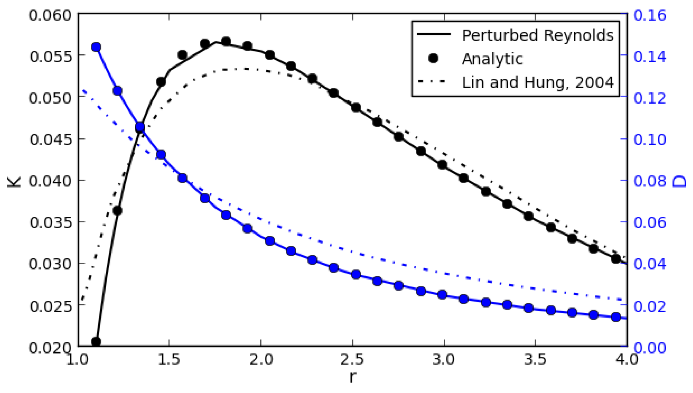
The stiffness and damping coefficients predicted using the perturbed Reynolds equation are verified by comparison with the results of Lin and Hung [13] as well as our analytic solution. In Figure 2, the dimensionless stiffness and damping coefficients are plotted over a range of taper ratios. The numerical solution of the perturbed Reynolds equation from the present work matches the analytic solution and confirms that discretization and iterative convergence errors are sufficiently small. The perturbed Reynolds equation results from the present work are comparable with [13] (which were also predicted using the perturbed Reynolds equation). Discrepancies in K and D are attributable to the method by which the results of Lin and Hung were extracted from the original paper [13]. K and D were extracted from a digitized version of a figure in the original paper and then scaled by a factor of six (to reconcile differences in non-dimensionalization).
7.2. Transient, Pure Squeeze Motion between Infinite Parallel Plates
As the sliding velocity of the linear slider bearing approaches zero () and the taper ratio approaches unity (), the flow within the infinitely long, linear slider bearing becomes that of flow between infinitely long, parallel plates. When the lower wall (“movingWall”) of the bearing is given a harmonic displacement normal to the sliding direction (y-direction), the flow becomes pure squeeze motion between infinitely long parallel plates. This type of flow may be viewed as the simplest type of transient flow that develops within a linear slider bearing, warranting it as the first test case to evaluate the dynamic coefficients using transient Reynolds and transient CFD with a moving boundary.
The same form of the dimensionless dynamic coefficients is applied to pure squeeze motion between parallel plates as to the linear slider bearing, while, for pure squeeze motion, the sliding velocity prescribed in the Reynolds equation and CFD models is zero, and a sliding velocity (other than zero) is nonetheless required as part of the non-dimensionalization of the dynamic coefficients. For pure squeeze motion between parallel plates, a sliding velocity (m s) (sliding velocity of linear bearing) is used within the non-dimensionalization of the dynamic coefficients to maintain consistency.
For pure squeeze motion between infinitely long, parallel plates, the transient Reynolds equation can be solved analytically and results in a dimensionless load given by Equation (30) San Andrés [31]:
The dynamic load predicted by the transient Reynolds equation and transient CFD with a moving boundary are both compared in Figure 3 against the analytic solution for the dynamic load offered by Equation (31).
In Figure 3, the numerical solution of the transient Reynolds equation (red dashed line) lies on top of the analytic solution given by Equation (31) (black solid circle). Using CFD with a moving boundary (Stokes and Navier–Stokes), the transient load does not match the analytic solution. While solutions of the Navier–Stokes equations (with inertia, black solid line) and the Stokes equations (without inertia, magenta square) result in dynamic loads comparable with each other, both differ in both magnitude and phase from the analytic solution. The dynamic load predicted using CFD with a moving boundary has a larger amplitude and lags the analytic, dynamic load. Since the CFD solution of the NSE and Stokes equations result in the same dynamic load, advective inertia effects for can be considered negligible.
The dynamic loads in Figure 3 can be used to estimate the dynamic properties of the squeeze film between the parallel plates. The analytic solution for the dynamic load results in zero stiffness and a dimensionless damping coefficient per unit length, . The time and frequency domain estimates based on the dynamic load from the transient Reynolds equation also result in zero stiffness and the same damping coefficient, . However, the dynamic load predicted by CFD with a moving boundary results in stiffness and damping coefficients, and , respectively, using both the time and frequency domain estimates. The time and frequency domain methods for estimating the dynamic coefficients described in the present work are verified through the accuracy of the damping coefficient predicted. There is negligible error when using the dynamic load from transient Reynolds to determine the damping coefficient. Additionally, the error is only % when dynamic load from CFD with a moving boundary is used to estimate the coefficients.
The non-zero value for K is not physically relevant. This is clear if we evaluate the change in force generated by the flow between parallel plates when the film thickness is subject to a small, finite displacement, . If the flow is steady, and the film thickness is , the load is zero, . If the film thickness is increased slightly, , the steady load will again be zero, . The stiffness can then be approximated as . In the case of pure squeeze motion between parallel plates, the stiffness K must be zero. A non-zero, non-physical value for K results because the dynamic model of the bearing is not correct for transient CFD with temporal inertia effects. In reality, it is not K that is being computed but the dynamic stiffness, . The temporal inertial effects must be captured through the addition of an added mass coefficient to the dynamic model.
The increased amplitude and phase lag in the dynamic load predicted by CFD with a moving boundary and the corresponding non-physical K result from temporal inertia effects. Temporal inertia effects arise due to the presence of the transient, or temporal inertial terms, , in the linear momentum conservation equations. Temporal inertia is present within the linear momentum equations of both the transient Navier–Stokes and transient Stokes equations—Equations (4) and (5), respectively. In pure squeeze flow, the oscillating lower boundary of the domain pushes and pulls on the fluid, causing it to accelerate and causing the acceleration, , within the linear momentum equation in the y-direction “activate”. Through the services of the continuity equation for the incompressible flow, the temporal inertia term in the y-direction activates the temporal inertia term in the x-direction of linear momentum, . As an example, consider the squeezing of an incompressible column of fluid situated between the parallel plates. As the fluid is squeezed, the column of fluid perpendicular to the direction of squeeze will have to expand in the x-direction in order to preserve volumetric and mass continuity. The phenomenon is akin to the Poisson ratio and the transverse contraction strain resulting from logitudinal extension strain. In the linear momentum equation in the x-direction, the additional fluid acceleration has to be balanced by an increase in the pressure gradient and subsequently an increase in the pressure and normal load (integrated pressure). By contrast, in the steady-state form of the linear momentum equation in the x-direction, the pressure gradient balances only the viscous shear.
One can therefore conclude that the net effect of the temporal inertia term on the flow between parallel plates (and by extension the flow in a linear slider bearing or any other bearing subject to the same effect) is to increase the magnitude of the dynamic load and change its phase. To account for the temporal inertia, it is necessary to modify the dynamic model of the slider bearing behavior. In addition to a spring and damper, a dimensionless added mass coefficient per unit length, (where m is the dimensional added mass per unit length), must be incorporated into the linear dynamic model of the total, transient, dimensionless bearing load per unit length, resulting in Equation (32):
Both the time domain and frequency domain estimates of the linearized dynamic coefficients (K, D, M) can be modified to include the added mass coefficient. The time domain estimate can be made by solving the overdetermined system, Equation (33), for the bearing parameters K, D, and M:
In the frequency domain, Equation (33) leads to the frequency response function given by Equation (34):
The particular form of the frequency response function given by Equation (34) is also known as the dynamic stiffness and consists of both real and imaginary components. The imaginary component can be used to determine the damping coefficients as introduced previously:
It is noteworthy, however, that the real component contains both the static stiffness and the added mass of the fluid within the bearing:
Equation (32) applies only to the dynamic load predicted by CFD with a moving boundary. The classical Reynolds equation (perturbed form or transient) has by initial assumption excluded temporal inertia as part of its derivation. As a result, there are no added mass effects within the load resulting from Reynolds equation and for that reason alone a spring-damper model should be used to model the bearing dynamic behavior in the present work. Added mass coefficients (inertia parameters) would be required if inertia effects were retained within the Reynolds equation as in Dousti [33].
Tichy and Modest [34] previously investigated discrepancies between CFD and Reynolds equation results for squeeze film flow between parallel and inclined plates. As in the present work, Tichy and Modest identified fluid inertia as the source of increased load amplitude predicted by CFD. However, the authors did not attempt to capture temporal inertia effects through an added mass coefficient within the dynamic model of the bearing.
For flow between parallel plates, the stiffness, K is zero and the added mass coefficient resulting from the temporal inertia of the fluid can be solved for directly. Using the dynamic models of the slider bearing described above and modified to account for temporal inertia effects, new estimates of the dynamic properties of squeeze flow between parallel plates using CFD with a moving boundary are made. The damping coefficient remains the same, (% larger than transient Reynolds), and the dimensionless, added mass coefficients per unit length predicted using time and frequency domain methods are and , respectively. As the Reynolds equation does not account for temporal inertia, the resulting dynamic load exhibits no added mass effects and the dynamic response of the fluid film subject to boundary oscillation is very different from that predicted by CFD.
The need to include an added mass coefficient to account for temporal inertia effects within the CFD-predicted loads is rather surprising. The reduced squeeze Reynolds number, , is comparatively small when viewed alongside the reduced sliding Reynolds number . While the present work supported the claim that advective inertia effects are negligible for , it seems that a different, and much smaller threshold reduced Reynolds number exists. The determination of a threshold value of is reserved for a subsequent paper.
7.3. Transient, Infinitely Long Linear Slider Bearing with Oscillating Boundary
The dynamic load of an infinitely long, linear slider bearing subject to harmonic oscillation perpendicular to the direction of sliding (harmonic squeeze motion) is plotted in Figure 4. The linear slider bearing has a taper ratio and is subject to a sliding velocity (m s), in addition to the motion of the oscillating boundary that oscillates at a frequency of 141 (rad s) and with an amplitude equal to 10% of .
As with the pure squeeze motion between parallel plates, in Figure 4, the dynamic load predicted by CFD with a moving boundary is markedly different than the dynamic load predicted by the transient Reynolds equation. Both the amplitude and the phase of the predicted dynamic loads differ, owing to the presence of temporal inertia within the CFD results. The dimensionless stiffness and damping coefficients predicted from the transient Reynolds force in Figure 4 are 0.056 and 0.053, respectively, using the time domain estimate. The frequency domain estimates of K and D from the transient Reynolds equation are 0.055 and 0.053, respectively. The analytic solution of the Reynolds equation predicts and . Differences between the transient Reynolds equation and analytic results for K and D are within errors associated with discretization and iterative convergence errors of the transient Reynolds equation numerical solution. In fact, the coincidence of the results is very good and reassuring in regard to the correctness of the methodology.
For the linear slider bearing dynamic model comprised only of a spring and damper; using the time domain estimation method, the dynamic force from CFD with a moving boundary (Figure 3) results in and . Evaluation of the stiffness and damping using the frequency domain method yields almost identical values of and , respectively. The negative direct stiffness coefficient is non-physical and results from the absence of an added mass coefficient within the dynamic model of the slider bearing. If an added mass coefficient is introduced in the dynamic model, the negative stiffness would make more sense since it would represent a component of the dynamic stiffness, , rather than just a static stiffness K. Note that, unlike for the pure squeeze motion between parallel plates, it is not possible to separate K and M from by just using a single forced oscillation frequency . It would be necessary to fit the stiffness and mass parameters, K and M, respectively, over a range of excitation frequencies . The determination of K and M from the quantity is the subject of a subsequent paper. However, it is noteworthy to mention that a preliminary investigation into resolving K and M separately from CFD with a moving boundary, determined that both dynamic parameters exhibit some excitation frequency dependence not predicted by Reynolds equation.
Table 1 summarizes K, D, and for the linear slider bearing at various taper ratios predicted by our analytic solution, as well as by the proposed frequency domain estimation method using the dynamic forces obtain through both the transient Reynolds equation and transient CFD with a moving boundary. K and D predicted by our analytic solution and transient Reynolds equation match exactly for higher taper ratios, while a 10%, difference in K manifests itself at the lowest taper ratio, .
For the CFD with a moving boundary, it was possible to directly compare the damping coefficients with our analytic and transient Reynolds equation predicted results. Generally, CFD with a moving boundary over-predicted the damping coefficient when compared to our analytic solution and transient Reynolds equation. For , CFD predicts a 6% higher D, while, for , the over-prediction rises to 104%. We believe that the CFD model predicts higher values than our analytic solution due to the increased role played by additional viscous terms present in the CFD model (Stokes equations vs. Reynolds equation). The additional viscous terms may increase energy dissipation results in higher values of D predicted by CFD with a moving boundary. In a subsequent paper, numerical errors will be directly quantified for the transient CFD with a moving boundary, and the role of additional viscous terms within the governing equations will be investigated.
8. Conclusions
Two methods for the estimation of the dynamic coefficients of slider bearings are introduced and the predicted dynamic coefficients compared. Both time and frequency domain methods predict dynamic coefficients that matched over the range of geometric and operational conditions considered. While the methods for evaluating the dynamic coefficients can be applied to the results from transient Reynolds equation or transient CFD with a moving boundary, some differences in both implementation and the predicted results are observed.
Most notably, for CFD cases:
- Temporal inertia is significant even for a reduced squeeze Reynolds number and subsequently requires the addition of an added mass coefficient to the dynamic model of the bearing.
- Advective inertia has a negligible impact on the steady-state and dynamic load of the linear slider bearing for a the reduced sliding Reynolds number ; this is consistent with the assumption of negligible advective inertia for as stated in Szeri [21].
- Threshold values for cannot be applied to in determining the influence of temporal inertia. Temporal inertia remains significant for numbers that are four orders of magnitude smaller than the threshold value for .
- The damping coefficient predicted for the linear slider bearing considered is higher than that predicted by our analytic solution or transient Reynolds equation. Relative differences in the predicted values of D are the largest for large taper ratios.
- Direct computation of K and M requires excitation of the bearing at multiple and preliminary results indicated a frequency dependence not exhibited by our analytic solution or transient Reynolds equation.
While the present work was applied to a linear slider bearing and pure squeeze flow between parallel plates, the proposed methodology for dynamic coefficient estimation is general and can be extended to complex journal bearings. While use of a perturbed Reynolds equation to determine the dynamic coefficients is computationally faster, the primary motivation is to be able to extract the dynamic coefficients from a CFD model of a bearing with complex geometric features and physics which are not easily, or even possible to be, incorporated into the Reynolds equation.
Author Contributions
Troy Snyder and Minel Braun contributed equally to writing the paper and development of the methods proposed therein.
Conflicts of Interest
The authors declare no conflict of interest.
Appendix A. Discrete Form of the Perturbed and Transient Reynolds Equations
Equation (11) is discretized using second-order, finite differences assuming constant grid spacing. This leads to the following linear system that can be solved for the dimensionless static pressure, :
Discretizing Equation (12) leads the following linear system that can be solved for the dimensionless pressure gradient with respect to , :
Discretizing Equation (13) leads the following linear system that can be solved for the dimensionless pressure gradient with respect to , :
Note that, for the perturbed Reynolds equation, the film thickness in the discrete form of the equations is the static film thickness, . In addition, for the perturbed Reynolds equation, n is the iterative index for the Gauss–Seidel method employed to solve the linear system of equations. Signs on the source terms in the discrete equations have been changed from those in the differential equations so positive stiffness and damping coefficients result from integration of and fields, respectively.
The transient Reynolds Equation (22) is also cast in discrete form using second-order finite differences. The following system of equations is solved until iterative convergence is reached at each time step:
After an iteratively converged pressure field is obtained by solving the linear system of equations above, the time step is advanced, which results in a new film thickness function, and the system of equations above is solved for the pressures at the new time step. In the transient system of equations, m denotes the time step and n denotes the Gauss–Seidel iteration within each time step.
In all of the discrete equations presented above, the under-relaxation parameter was used to ensure stability of the computations. The particular value of the under- relaxation parameter is not optimal and motivated solely by the typical value of under-relaxation parameters used in solving the incompressible linear momentum equations in CFD. Computational time involved in solving the Reynolds equation was not a concern so an optimal value of the relaxation parameter (under- or over-relaxation) was not investigated.
References
- Tiwari, R.; Lees, A.W.; Friswell, M.I. Identification of dynamic bearing parameters: A review. Shock Vib. Dig. 2004, 36, 99–124. [Google Scholar] [CrossRef]
- Snyder, W.T. The Nonlinear Hydrodynamic Slider Bearing. J. Basic Eng. 1963, 85, 429–433. [Google Scholar] [CrossRef]
- Osterle, J.F.; Chou, Y.T.; Saibel, E.A. Effect of Lubricant Inertia in Journal-Bearing Lubrication. J. Appl. Mech. 1957, 24, 494–496. [Google Scholar]
- Osterle, J.F.; Hughes, W.F. The effect of lubricant inertia in hydrostatic thrust-bearing lubrication. Wear 1958, 1, 465–471. [Google Scholar] [CrossRef]
- Osterle, J.F.; Hughes, W.F. High speed effects in pneumodynamic journal bearing lubrication. Appl. Sci. Res. 1958, 7, 89–99. [Google Scholar] [CrossRef]
- Launder, B.E.; Leschziner, M. Flow in Finite-Width, Thrust Bearings Including Inertial Effects: I— Laminar Flow. J. Lubr. Technol. 1978, 100, 330–338. [Google Scholar] [CrossRef]
- Patankar, S.V.; Spalding, D.B. Numerical Predictions of Three-Dimensional Flows; Technical Report MED Rep. EF/TN/A/46; Imperial College: London, UK, 1972. [Google Scholar]
- Chen, P.Y.P.; Hahn, E.J. Use of computational fluid dynamics in hydrodynamic lubrication. J. Eng. Tribol. 1998, 212, 427–436. [Google Scholar] [CrossRef]
- Dobrica, M.; Fillon, M. Reynolds’ Model Suitability in Simulating Rayleigh Step Bearing Thermohydrodynamic Problems. Tribol. Trans. 2005, 48, 522–530. [Google Scholar] [CrossRef]
- Vakilian, M.; Gandjalikhan Nassab, S.A.; Kheirandish, Z. CFD-Based Thermohydrodynamic Analysis of Rayleigh Step Bearings Considering an Inertia Effect. Tribol. Trans. 2014, 57, 123–133. [Google Scholar] [CrossRef]
- Fouflias, D.G.; Charitopoulos, A.G.; Papadopoulos, C.I.; Kaiktsis, L.; Fillon, M. Performance comparison between textured, pocket, and tapered-land sector-pad thrust bearings using computational fluid dynamics thermohydrodynamic analysis. J. Eng. Tribol. 2015, 229, 376–397. [Google Scholar] [CrossRef]
- Zeng, Q.H.; Chen, L.S.; Bogy, D.B. A modal analysis method for slider-air bearings in hard disk drives. IEEE Trans. Magn. 1997, 33, 3124–3126. [Google Scholar] [CrossRef]
- Lin, J.R.; Hung, C.R. Analysis of dynamic characteristics for wide slider bearings with an exponential film profile. J. Mar. Sci. Technol. 2004, 12, 217–221. [Google Scholar]
- Lin, J.R.; Lu, R.F.; Hung, C.R. Dynamic characteristics of wide exponential film-shape slider bearings lubricated with a non-Newtonian couple stress fluid. J. Mar. Sci. Technol. 2006, 14, 93–101. [Google Scholar]
- Lin, J.R.; Hung, C.R.; Hsu, C.H.; Lai, C. Dynamic stiffness and damping characteristics of one-dimensional magneto-hydrodynamic inclined-plane slider bearings. J. Eng. Tribol. 2009, 223, 211–219. [Google Scholar] [CrossRef]
- Naduvinamani, N.B.; Marali, G.B. Dynamic Reynolds equation for micropolar fluids and the analysis of plane inclined slider bearings with squeezing effect. J. Eng. Tribol. 2007, 221, 823–829. [Google Scholar] [CrossRef]
- Hanumagowda, B.N.; Gonchigara, T.; Kumar, J.S.; ShivaKumar, H.M. Steady and dynamics characteristics of MHD Land-Tapered slider bearing: Use of Stoke-Couplestress Model. Int. J. Pure Appl. Math. 2017, 113, 325–333. [Google Scholar]
- Lund, J.W.; Thomsen, K.K. A Calculation Method and Data for the Dynamic Coefficients of Oil-Lubricated Journal Bearings. In Topics in Fluid Film Bearing and Rotor Bearing System Design and Optimization; ASME: New York, NY, USA, 1978; pp. 1–28. [Google Scholar]
- Lund, J.W. Review of the Concept of Dynamic Coefficients for Fluid Film Journal bearings. J. Tribol. 1987, 109, 37–41. [Google Scholar] [CrossRef]
- Horvat, F.; Duramax Marine, Hiram, OH, USA. Personal communication, February 2016.
- Szeri, A. Fluid Film Lubrication, 2nd ed.; Cambridge University Press: Cambridge, UK, 2011; p. 254. [Google Scholar]
- Frene, J. Tapered Land Thrust Bearing Operating in Both Laminar and Turbulent Regimes. ASLE Trans. 1978, 21, 243–249. [Google Scholar] [CrossRef]
- Tannehill, J.C.; Anderson, D.A.; Pletcher, R.H. Computational Fluid Mechanics and Heat Transfer, 2nd ed.; Taylor & Francis: Didcot, UK, 1997. [Google Scholar]
- Braun, M.J.; Hannon, W.M. Cavitation formation and modelling for fluid film bearings: A review. J. Eng. Tribol. 2010, 224, 839–863. [Google Scholar] [CrossRef]
- White, F.M. Viscous Fluid Flow; McGraw-Hill: New York, NY, USA, 1991; p. 614. [Google Scholar]
- Münch, C.; Ausoni, P.; Braun, O.; Farhat, M.; Avellan, F. Fluid—Structure coupling for an oscillating hydrofoil. J. Fluids Struct. 2010, 26, 1018–1033. [Google Scholar] [CrossRef]
- Weller, H.G.; Tabor, G.; Jasak, H.; Fureby, C. A tensorial approach to computational continuum mechanics using object-oriented techniques. Comput. Phys. 1998, 12, 620–631. [Google Scholar] [CrossRef]
- Patankar, S.V. Numerical Heat Transfer and Fluid Flow; CRC Press: Boca Raton, FL, USA, 1980. [Google Scholar]
- Issa, R. Solution of the implicitly discretised fluid flow equations by operator-splitting. J. Comput. Phys. 1986, 62, 40–65. [Google Scholar] [CrossRef]
- Rhie, C.M.; Chow, W.L. Numerical study of the turbulent flow past an airfoil with trailing edge separation. AIAA J. 1983, 21, 1525–1532. [Google Scholar] [CrossRef]
- San Andrés, L. Modern Lubrication Theory. Classical Lubrication Theory, Notes 02. Texas A&M Digital Libraries. Available online: http://oaktrust.library.tamu.edu/handle/1969.1/93197 (accessed on June 2017).
- Celik, I.B.; Ghia, U.; Roache, P.J.; Freitas, C.J.; Coleman, H.; Raad, P.E. Procedure for Estimation and Reporting of Uncertainty Due to Discretization in CFD Applications. J. Fluids Eng. 2008, 130, 78001. [Google Scholar] [CrossRef]
- Dousti, S.; Cao, J.; Younan, A.; Allaire, P.; Dimond, T. Temporal and Convective Inertia Effects in Plain Journal Bearings With Eccentricity, Velocity and Acceleration. J. Tribol. 2012, 134, 031704. [Google Scholar] [CrossRef]
- Tichy, J.A.; Modest, M.F. Squeeze Film Flow between Arbitrary Two-Dimensional Surfaces Subject to Normal Oscillations. J. Lubr. Technol. 1978, 100, 316. [Google Scholar] [CrossRef]
Figure 1.
Geometry of infinitely long linear slider bearing subject to sliding and squeeze motion. When and , the geometry corresponds to pure squeeze motion between parallel plates.
Figure 1.
Geometry of infinitely long linear slider bearing subject to sliding and squeeze motion. When and , the geometry corresponds to pure squeeze motion between parallel plates.
Figure 2.
Comparison of dimensionless stiffness and damping coefficients of the linear slider bearing predicted by our numerical solution of the perturbed Reynolds equation, our analytic solution, and Lin and Hung [13]. K is in black (-axis) and D (-axis) are in blue with the solid lines indicating the present work, circle markers only indicating the analytic solution, and dashed-dotted lines indicating results extracted from [13]. The reduced sliding Reynolds number is

Figure 3.
Dimensionless, transient load generated fluid between two infinitely long parallel plates subject to pure squeeze motion (harmonic), and . Comparison between transient Reynolds equation (solved numerically), CFD with a moving boundary (Stokes and Navier–Stokes in the graph), and the analytic solution given by Equation (31). Dimensionless displacement, Y, is in blue and plotted along the -axis. The remaining curves are dimensionless load and are plotted along the -axis.
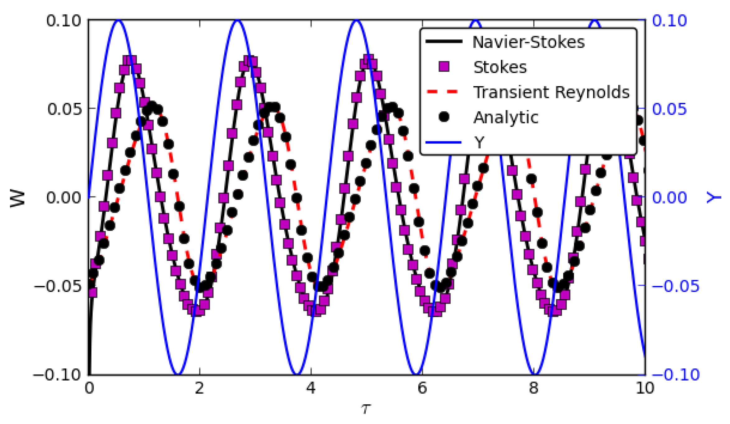
Figure 4.
Dimensionless, transient load generated by an infinitely long linear slider bearing subject to squeeze motion (harmonic), and . Comparison between transient Reynolds equation (solved numerically) and CFD with a moving boundary (Stokes). Dimensionless displacement, Y, is in blue and plotted along the -axis. The remaining curves are dimensionless load and are plotted along the -axis. Taper ratio, .

Table 1.
Dimensionless, dynamic bearing coefficients predicted using transient Reynolds equation, CFD with a moving boundary, and analytic solution of Reynolds equation. Dynamic coefficients are estimated using the frequency domain method.
Table 1.
Dimensionless, dynamic bearing coefficients predicted using transient Reynolds equation, CFD with a moving boundary, and analytic solution of Reynolds equation. Dynamic coefficients are estimated using the frequency domain method.
| Taper Ratio | Analytic | Transient Reynolds | CFD w/Moving Boundary | |||
|---|---|---|---|---|---|---|
| 1.1 | 0.021 | 0.144 | 0.019 | 0.146 | −0.435 | 0.152 |
| 1.5 | 0.053 | 0.087 | 0.053 | 0.088 | −0.331 | 0.101 |
| 2.0 | 0.056 | 0.053 | 0.055 | 0.053 | −0.433 | 0.060 |
| 2.5 | 0.049 | 0.035 | 0.049 | 0.035 | −0.231 | 0.056 |
| 3.0 | 0.042 | 0.025 | 0.042 | 0.025 | −0.214 | 0.051 |
© 2018 by the authors. Licensee MDPI, Basel, Switzerland. This article is an open access article distributed under the terms and conditions of the Creative Commons Attribution (CC BY) license (http://creativecommons.org/licenses/by/4.0/).
Share and Cite
MDPI and ACS Style
Snyder, T.; Braun, M. Comparison of Perturbed Reynolds Equation and CFD Models for the Prediction of Dynamic Coefficients of Sliding Bearings. Lubricants 2018, 6, 5. https://doi.org/10.3390/lubricants6010005
AMA Style
Snyder T, Braun M. Comparison of Perturbed Reynolds Equation and CFD Models for the Prediction of Dynamic Coefficients of Sliding Bearings. Lubricants. 2018; 6(1):5. https://doi.org/10.3390/lubricants6010005
Chicago/Turabian StyleSnyder, Troy, and Minel Braun. 2018. "Comparison of Perturbed Reynolds Equation and CFD Models for the Prediction of Dynamic Coefficients of Sliding Bearings" Lubricants 6, no. 1: 5. https://doi.org/10.3390/lubricants6010005
Note that from the first issue of 2016, this journal uses article numbers instead of page numbers. See further details here.