Importance of Emulsification in Calibrating Infrared Spectroscopes for Analyzing Water Contamination in Used or In-Service Engine Oil

Abstract

Using Fourier transform infrared (FT-IR) spectroscopy we investigated the water content of SAE 15W–40 diesel engine lubricating oil at various levels of contamination to establish instrument calibration standards for measuring water contamination in used or in-service engine oil by the standards of ASTM International. Since some known additives in consumer grade engine oil possess slightly hydrophilic properties, this experiment avoided changing the sample matrix with supplemental additives, such as adding surfactants, to achieve homogeneity of the original sample. The impact of sampling time after contamination on the spectral absorption signature was examined in an attempt to improve the accuracy of water contamination quantification and determine if water-soluble potassium bromide (KBr) windows were suitable for analyzing water in oil emulsions. Analysis of variance (ANOVA) modeling and limit of detection calculations were used to predict the ability to discriminate contamination levels over time. Our results revealed that the amount of water concentration in engine oil could be misinterpreted depending on the timing of the FT-IR measurement of the calibration standard after initial water contamination. Also, KBr windows are not sufficiently etched due to the limited window interaction with water molecules within micelles of emulsions to alter FT-IR spectral signatures.

1. Introduction

Typically, water does not mix readily with oil in any significant quantity due to the polar nature of water and the nonpolar nature of hydrocarbons; the attraction between water and oil molecules is far less than the attraction between two water molecules [1]. However, base engine oils are supplemented with additives. In particular, detergent additives interact and emulsify water. Zinc dialkyldithiophosphates (ZDDP) that are added for their anti-wear properties are also known to increase the saturation point of water in engine oil [2]. Water contamination in conventional engine lubricants can exist in a combination of three different states: free water, dissolved in oil, or as an emulsion [3]. Water can exist in a dissolved state (soluble form) with no visual indication until it reaches its saturation point dependent upon temperature, oil additives, and the age of the oil [3]. The presence of water in a dissolved state is due to engine oil being slightly hygroscopic [4] and is typically not seen as critically harmful to most components [5]. Water/oil emulsions can exist anywhere from 100 to 1000 ppm depending on the additives present, and the water/oil droplets in the emulsion can range from nanoemulsions (sub-100 nm) to microemulsions (10 µm) [6,7]. Free water consists of water droplets not dispersed or mixed with the oil and is second only to emulsions in being harmful to lubricated components, but is more easily separated from the oil than an emulsion [5]. Agitation, heat, and pressure caused by oil circulating through an engine will emulsify the water contaminate over time. While free water may exist at the bottom of an engine oil sump, common sampling procedures intentionally avoid sampling this area [8]. As a result, water in an engine oil sample primarily exists in dissolved or emulsified states, with dissolved water in concentrations as low as 50 ppm until it reaches the engine oil’s saturation point at which time droplet or micelle formation can occur [9].

Various efforts have been made to measure the water contamination of engine oil using different techniques. In 1965, researchers reported the possibility of using an infrared spectrophotometer to determine water contamination in engine oil by relating percent water in oil to absorbance per cm in the 2.9 µm band based on differential infrared analysis [10]. Mid-infrared spectroscopy in the attenuated total reflectance mode was successfully used to relate water band (3100–3700 cm⁻¹) absorption to up to 2.6% water content in marine lubricating oil samples using partial least squares regression [11]. With near-infrared spectroscopy, the water band was readily seen due to the changes in dipole moments under stimulation of light and hydrogen, being the least massive of atoms, experiences the greatest vibrations as seen with the O–H bond [12]. Interval partial least squares regression (iPLS) applied to FT-IR results of water in oil found the interval 3598–3732 cm⁻¹ resulted in the best prediction of water contamination [13]. Photoacoustic spectroscopy at 2.93 µm has been successfully used to detect water in oil with detection limits better than FT-IR [14]. A micro-acoustic sensor was used for water/oil emulsions and found the presence of water in engine oil caused an overall slight decrease in oil viscosity of up to 2% at 20% water concentration [15]. FT-IR analysis has been used to compare the properties of new and used engine oil to determine the feasibility of reconditioning the used oil as a dispersant in coal–water slurry fuel oils [16]. Terahertz time-domain spectroscopy has been used to discriminate among relatively low water concentrations (0%, 1%, 2% v/v) in conventional diesel engine oil with statistically significant differences among the water levels [17]. Also, nuclear magnetic resonance (NMR) spectroscopy has been used for various studies including studying the degradation of engine oil [18] analysis of the water content in chicken eggshells [19], detection of oil contamination in water [20], etc. With the decrease in cost and size, NMR devices have the potential to replace the more common methods of detection.

There are a number of commercially available methods for the testing of water in engine oil. One of these is the crackle test where a sample of oil is heated slightly above 100 °C to watch and listen for the boiling of water [2]. Other commercially available methods include a stoichiometric test by mixing the sample with calcium hydride in a pressurized vessel [9,21,22], the Karl Fischer coulometric titration (ASTM D6304, West Conshohocken, PA, USA) method of measuring the oxidation of sulfur dioxide by iodine and water [9,21,22], relative humidity testers that cannot measure free or emulsified water [9,21], and FT-IR analysis that can measure dissolved, free, and emulsified water and correlates well with the Karl Fischer method [9,22,23]. ASTM International (ASTM) has established FT-IR standards of practice for testing water contamination in used or in-service engine oil [24].

Water/oil emulsification takes time due to the strong cohesiveness of water molecules and the limited intermingling they have with the slightly polar end of some oil additives. This, in turn, affects the detectability of moisture content with FT-IR. Also, a demulsifying process can occur over a very extended period as some encapsulated water molecules are less kinetically stable than others. Analyses of the time it takes emulsifying agents to react at the water/oil interface in oils used by the pharmaceutical, food, and cosmetic industries have been performed to improve emulsifier selection for those industries [25]. Also, a number of studies within the petroleum industry have examined the opposite effect, the stability of water/oil emulsions, and the rate of demulsification [26,27,28,29,30,31,32]. Obtaining a complete emulsion of water in oil may be critical to accurate and repeatable FT-IR measurements of water in oil. ASTM E2412–10 [25] did not include consistent specifics on the mixing of a sample before FT-IR analysis. The main body of the standard indicates that samples be shaken or agitated to ensure a representative sample, while the second annex specifies mixing, sonicating, or mechanical shaking for at least 15 min [25]. Researchers have approached the water/oil emulsion differently. Some researchers have specified mixing samples to obtain emulsion [4,17], while others did not specify. Other researchers have minimized mixing to obtain water/oil emulsions with additional detergent additives [13]. Differences in the emulsion state of water in oil may impact FT-IR results. Attempting to sample free water directly from the bottom or even falling within the oil column does not ensure a strong correlation with actual water concentration in oil. Emulsified water/oil best represents the state of a water-contaminated oil sample removed from an engine. A sufficiently stable, emulsified sample with infrared-absorbing micelles helps reduce the variability of measurements caused by the scattering of infrared light by larger water droplets [33].

No studies have focused on understanding the time lag of freshly contaminated oil to form a complete emulsion in creating calibration samples for accurate FT-IR measurement. We investigated the capability of FT-IR techniques to distinguish eight levels (0%, 0.1%, 0.2%, 0.5%, 1%, 2%, 5%, and 10% v/v) of water contamination of fresh diesel engine oil and to determine if this capability changes over time due to the rate of a water/oil interaction.

2. Material and Methods

2.1. Sample Preparation

A container (946 mL) of a common diesel engine oil (SAE 15W–40, Shell Rotella T) was purchased from a domestic retail market in Carbondale, IL, USA. A pipette was used to place 8-ml samples of this fresh oil into each of 16 clear glass vials (in accordance with ASTM standards [24]) that were approximately 15 mm in diameter and 47 mm in height. The treatments included different water proportions that contaminated the fresh engine oil (0%, 0.1%, 0.2%, 0.5%, 1%, 2%, 5%, and 10% v/v).

The contaminating process was performed by replacing the appropriate volume of oil with the same amount of distilled water using a pipette. For example, 8 µL of oil was removed and 8 µL of water was added for 0.1% water contamination samples. Different volumes of 16 µL, 40 µL, 80 µL, 160 µL, 400 µL, and 800 µL were used for the other water contamination levels of 0.2%, 0.5%, 1%, 2%, 5%, and 10%, respectively. Two samples of each water contamination level and two control samples of 0% contamination were prepared for a total of 16 samples. At week 0 and for each subsequent week’s measurement, each prepared sample, including the noncontaminated sample, was agitated for about two hours (a minimum of 15 min of agitation is recommended by ASTM International standards for in-service oils [24]) with a rotary device and left for about 24 h before performing the FT-IR analysis to allow any air bubbles formed during agitation to disperse and for free water to settle. In creating a calibration standard, the goal is to create the most stable and consistently reliable contaminant concentration, hence the wait time to allow for only the emulsion particles with long-term stability [34] to remain in the oil matrix before FT-IR testing. The aim of agitating the oil samples was to obtain a relatively consistent homogeneity in the samples each time before testing. Each sample was stored in a closed vial and left standing upright in a closed box to prevent photo-degradation apart from when a vial would temporarily be removed for sampling for FT-IR analysis, shaking, or having a photo taken to track any change in color.

2.2. FT-IR Spectral Analysis

The infrared spectra were recorded with a wavenumber range of 400 to 4000 cm⁻¹ with an FT-IR spectrometer (Thermo-Nicolet Nexus 670, Waltham, MA, USA). The system was purged with dry air before each measurement (background or sample) to minimize interference from atmospheric moisture. A background measurement, KBr windows alone, was taken before measuring each sample. A 3 µL portion of the respective sample was pipetted from the vertical and horizontal center of the vial onto a 1-inch diameter KBr window and a similar window was placed atop the first and rotated 90 degrees to ensure the oil was spread evenly over the windows’ faces—aligning the same window faces with one another in the same orientation as noted by marks made on the edge of each window that were also aligned with a notch in the sample holder that was inserted in the FT-IR in the same orientation each time, such that the general crystalline structure’s alignment had reasonable uniformity throughout the tests. The KBr/oil sample was placed in a sample tray with a polytetrafluoroethylene (PTFE) ring sized to ensure the windows were in the same physical orientation and location in the sample holder each time the experiment was performed to reduce the possibility of differences in the refraction of light between each measurement. By gathering the spectra from the same location of the KBr window during the measurement of the background or sample, spatial dependent spectra were minimized. After each sample was prepared in a KBr window, two consecutive spectra measurements were recorded. The KBr windows were cleaned with methylene chloride after each sample was tested.

The ASTM standards note that KBr windows can be used without the necessary fringe corrections that would be required for zinc selenide (ZnSe) windows. However, it cautions that KBr window cells are prone to water damage [24]. For testing the reliability of KBr windows (KBr being widely available, economical, and offering an excellent transmission band across the IR spectrum), an oil sample with the highest concentration of water contamination (10% in the stable emulsion, week 9) was used to run successive spectral acquisitions. After the 3 µL portion (emulsified water-in-oil sample) was pipetted onto the KBr windows as previously described (providing a typical path length of approximately 0.01 mm), the system was purged with dry air prior for about 3 minutes, and then at least two spectra were collected. Afterward, the sample holder (including the KBr windows with sample) was moved from the usual upright position and allowed to rest horizontally in the dry ambient air (inside the FT-IR) for an extended water-in-oil emulsion on KBr windows exposure time of 30 min. Again, after repositioning and purging following the elapsed time, more spectra were acquired from the extended exposure time of KBr windows on the water-in-oil emulsion. The windows were cleaned as previously mentioned and spectra of fresh samples were collected.

The aforementioned procedures were repeated for the extended exposure times of 60 min and 90 min for the two subsequent trials. This entire procedure was also performed once again on the same KBr windows as well as on a different set of KBr windows.

As for testing the emulsification of diesel engine oil over time through mechanical agitation without the addition of supplementary emulsifying agents, thirty-two spectra measurements (2 for each of the 16 samples) were completed weekly for five consecutive weeks starting from week 0 (the day after oil contamination) to week 4. The similar FT-IR analysis was followed at week 6, 9, and 14. The amplitude of water’s O–H stretching band (approximately 3000–3800 cm⁻¹) was used for spectral analysis. The amplitude of the signal peak was determined from a two-point baseline as stated in the ASTM standards [24].

2.3. Data Preprocessing and Analysis

Before analysis, FT-IR spectra were inspected and discarded if the intensities in the region of 2900 cm⁻¹ to 2940 cm⁻¹ were higher than the absorbance threshold of 2.5 a.u. to avoid any saturation effects in the measurement. Prior to statistical analysis of the area of the wavenumber range of the O–H stretching band (from 3150 to 3500 cm⁻¹), the baselines of each whole spectrum were adjusted to minimize effects of baseline shifting between FT-IR measurement. As similarly established with the ASTM standards, the end of the spectral range [24] (3970 to 3995 cm⁻¹) where each spectrum flattens due to the lack of any detectable signals was shifted to zero on the absorbance scale, and the same shift was applied to the entire baseline of each respective spectrum.

Each of the four spectra measurements for each water contamination level for each week were treated as replications [35]. Analysis of variance (ANOVA) was used to determine if there was a significant difference (α = 0.05) in absorbance among the water contamination levels for each week of measurements and Fisher’s least significant difference (LSD) was used to determine significance among contamination levels. Regression analysis was completed using absorbance to predict water contamination using data from each week. The linear models were evaluated on the coefficient of determination (R²).

To determine the smallest concentration of water that can be measured by FT-IR, the amplitude of the entire broad peak water signal around the 3400 cm⁻¹ wavenumber was used for relative comparison over time [36]. The amplitudes of water absorbance were found by Gaussian curve fitting after eliminating the continuum background. The peak amplitude from each of these was plotted over time. The mean of two measurements for each sample was used to find the amplitudes of the water signature for each respective sample with the exception being if a measurement was discarded.

Water absorbance amplitudes versus water concentration were used to quantify the limit of detection (LOD) and limit of quantification (LOQ) [37] for water concentrations in oil by FT-IR spectral analysis. LOD and LOQ were calculated from a linear regression fit, where $\mathrm{LOD}=3.3\frac{S_a}{b}$ and $\mathrm{LOQ}=10\frac{S_a}{b}$. Here, S_a is the standard deviation of the response estimated from y-intercepts of each respective regression line, and b is the slope. The results of the ANOVA and LOD methods were compared.

3. Results

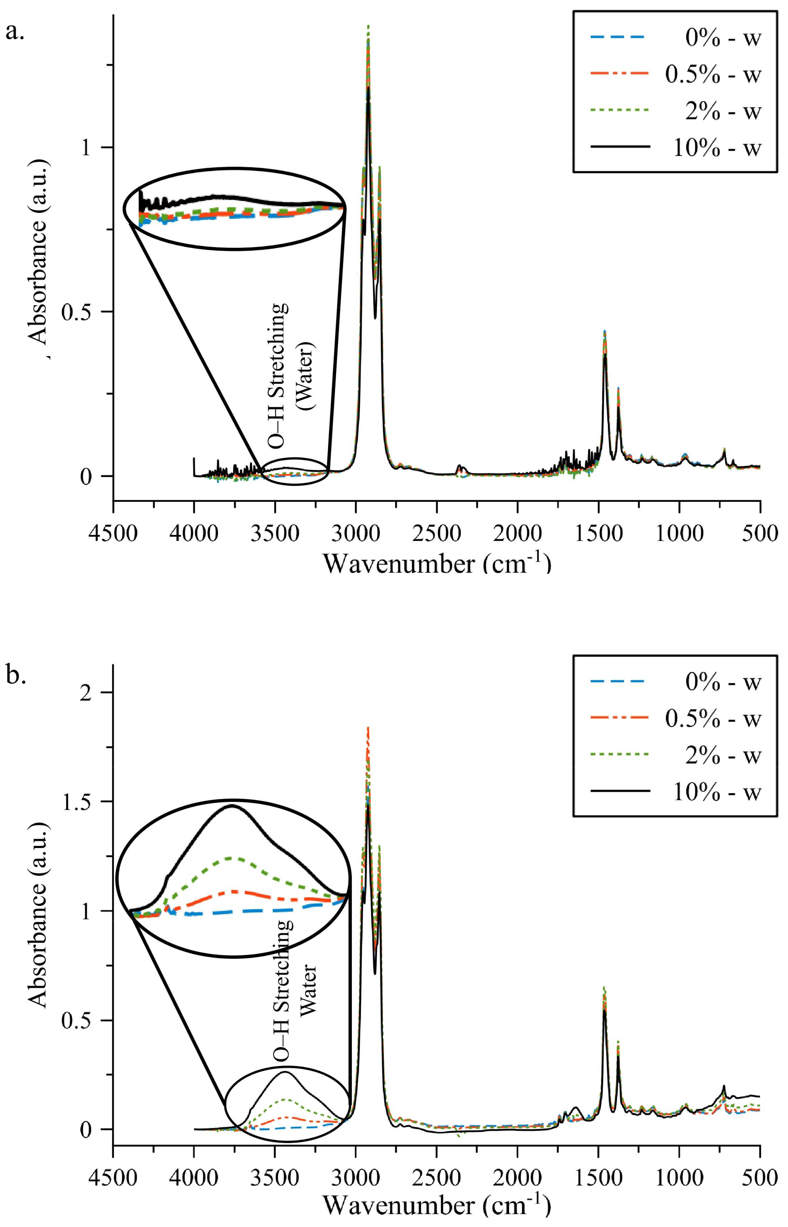
3.1. FT-IR Absorption Spectra

The variability in spectral signatures from water-soluble KBr windows due to even the highest concentration of 10% water in oil emulsion was negligible as seen in Figure 1.

The mean amplitude of the O–H stretching band was plotted versus the exposure time of the KBr windows to the water/oil emulsion. In case one argues that the cleaning process polishes the windows, the plot does not reflect the additive total exposure time, but merely the time an individual sample sat sandwiched between the windows during the purge process, spectral acquisition, and the purposefully extended exposure time. The mean peak amplitudes of the water signature throughout the KBr usability tests were comparable to the week 9 values as will be demonstrated later in Figure 3, yet the windows’ solubility to water was not a critical factor in spectral acquisition even after extended exposure time. In fact, the mean value of the peak water amplitudes taken of the fresh sample after the additional 3 days of exposure had a value of 0.2089 ± 0.03 a.u., which is indeed within the expected range as would be anticipated by examining Figure 1. The spectral signatures seem to be less affected by a water/oil emulsion exposure to water-soluble KBr windows than indeterminate errors such as sampling differences, background gas, and instrument noise that can affect the experimental results.

FT-IR absorbance spectra in the O–H stretching band changed over time, with little difference among water concentrations one day after contamination (week 0) to noticeable differences at week 9 (Figure 2).

The mean of the amplitudes for the peak water absorbance of the samples was plotted for each water contamination level over time to depict the increased interaction and detectability of the water/oil mixture, as seen in Figure 3. The minuscule values for the 0% appeared quite random and showed no correlations (i.e., low R-squared value) over weeks. The 0.1%, while not as random, was still out of the limit of detection for the instrument. However, the higher value of R-squared for the concentration from 0.2% to 10% shows a strong correlation change of water content in oil over weeks as 2nd order polynomials.

The linear representation of absorbance vs. percent water concentration was depicted in Figure 4.

FT-IR analysis of different concentrations of water contamination in diesel engine oil demonstrated an increasing ability to detect low-level concentrations of contamination over time. As the time interval increased on a weekly basis, the water molecules increasingly interacted with the oil and additives and became more dispersed throughout the oil column and more likely to be probed by the pipette for FT-IR analysis. The linear representation of absorbance vs. percent concentration (as depicted in Figure 4) was similar to the fifth figure in the Frassa study [10], but we have multiple weeks represented. The separation between week 4 and week 6 can, in part, be explained by no data collection being taken at week 5. The fact that the remaining free water was dwindling as it entered a stable emulsification led to a plateauing of average absorbance values after week 6 as is seen in Figure 3. This is also evident in Figure 4 by the fact that week 6 through 14 become more minimally spaced.

The 5% and 10% water contaminations had noticeably larger amplitudes than the 0% control at day one. While the 10% concentration was readily detectable as having water on day one, the amplitudes of the water-contaminated samples rose over time and most started to become different from each other starting from week 2, before beginning to plateau around week 9 as the water reached a maximum dispersal as an emulsion. This dispersive effect can be witnessed over time as a milky emulsion. The graph suggests that by week 4 and week 9 the 0.2% and 0.1% concentrations should be discernible respectively; however, with the variability in the amplitudes and the similarity to the control’s amplitude, one cannot safely make that argument as shown with the LOD. After week 9, it is suspected that Ostwald ripening may start to make the emulsion unstable causing a phase separation as some downward trending in water absorbance signatures has already started taking place [38]. As Ostwald ripening occurs and the droplet size increases this can increase the scattering of incident light which in turn decreases the extinction coefficient for the test sample. This is in accordance with Mie theory for droplet sizes from 1 to 100 µm where the index of refraction has a larger contribution than does the particle size [39,40]. This in part may explain the variability that is especially seen in the higher concentration of 10% contamination as the initially large water droplet is dispersed into a varied distribution of particle sizes, some potentially much larger than others, yet fewer in number [41]. A sampling size of 3 µL may be too small to guarantee a true representative sample of this size distribution yielding in some cases greater numbers of larger droplets that scatter light, reducing the extinction coefficient and in turn reducing the absorbance signatures. More replications and larger sample sizes may reduce this variation. A larger sample size and an increased path length could also yield a better LOD.

3.2. ANOVA Modeling

Differences between the area of the FT-IR absorbance measurement of each contaminated oil sample and the area of the mean of noncontaminated samples in the 3150–3500 wavenumber range were summarized in

Table 1. Summary of differences from 0.0% contamination of the mean absorbance of water contamination levels of the area of the 3150-3500 wavenumber range for each week.

Water Contamination (%)	Week 0		Week 1		Week 2		Week 3		Week 4		Week 6		Week 9		Week 14
	N	Mean *	N	Mean *	N	Mean *	N	Mean *	N	Mean *	N	Mean *	N	Mean *	N	Mean *
0.1	4	−0.105 c	3	−1.022 e	4	1.862 e	3	1.080e	4	3.097 e	4	−0.989 e	4	2.893 d	4	−0.327 f
0.2	4	0.064 bc	2	1.204 de	4	2.241 e	4	0.703 e	4	4.629 e	4	1.424 e	4	7.836 d	4	3.635 ef
0.5	4	1.603 bc	4	1.380 d	4	6.721 d	4	4.711 d	4	6.491 d	2	9.020 cd	4	7.646 d	4	8.005 e
1.0	4	3.194ab	4	4.021 c	2	9.708 c	4	7.688 c	4	10.050 cd	3	15.499 c	4	17.119 c	4	21.587 d
2.0	2	3.187abc	2	5.324 c	4	11.430 bc	4	9.063 c	4	12.476 c	4	30.321 b	4	33.977 b	4	32.068 c
5.0	4	1.724 bc	4	8.638 b	4	12.442 b	4	11.589 b	4	18.973 b	3	32.941 b	4	40.638 b	4	39.968 b
10.0	4	6.273a	3	15.323a	4	22.977a	4	30.822a	4	29.497a	4	63.018a	4	58.597a	4	54.629a

* Means in each column with the same letter are not significantly differen.

, indicating the number of significant differences among the contamination levels. At week 0 (1 day after contamination and mixing), the only significant difference was that 10% was higher than the lower concentration levels (0.5–0.1%). At week 1, 10% and 5% were significantly different from each other and from all other levels, and although there was no difference in 1% and 2%, they were significantly different from all other levels. At week 2, 0.5% was also distinguishable from all other levels. The significant differences among the contamination levels were similar for weeks 2 through 14. Week 14 had the most significant differences among contamination levels, with 10%, 5%, 2%, and 1% different from each other and all other levels. The lowest two contamination levels of 0.1% and 0.2% were not distinguishable at any week.

Generally, the mean absorbance for a given contamination level increased over time with some plateauing about week 9.

Table 2. Summary of mean absorbance of water contamination levels of the area of the 3150-3500 wavenumber range for each week using ANOVA analysis.

Week	0.5%		1.0%		2.0%
	N	Mean *	N	Mean *	N	Mean *
14	3	8.005a	4	21.587a	4	32.068a
9	4	7.646a	4	17.119 b	4	33.977a
6	2	9.019a	3	15.49 b	4	30.321a
4	4	6.491a	4	10.050 c	4	12.476 b
3	4	4.711ab	4	7.688 cd	4	9.063 bc
2	4	6.721a	2	9.708 c	4	11.429 b
1	4	1.380 b	4	4.021 de	2	5.324 bc
0	4	1.603 b	4	3.194 e	2	3.187 c

* Means in each column with the same letter are not significantly different.

summarizes the changes in absorbance by week for contamination rates of 0.5%, 1%, and 2%. For 0.5%, absorbance for week 0 and 1 was significantly lower than all other weeks except week 3. For 1%, week 14 had the significantly highest absorbance, with weeks 6 and 9 significantly different from the other weeks. For the 2% rate, absorbance at weeks 6, 9, and 14 were significantly higher than the other weeks.

The difference in the absorbance values between each contamination level and the noncontaminated sample changed each week, indicating an increase in detectable water in the samples over time, as also evidenced by a change in color from the typical amber color of new engine oil to a milky color. This change was most likely a change in the amount of water in complete emulsion with the oil.

3.3. Predicting Water Contamination Level from FT-IR Absorption Spectra Analysis

The LOD and LOQ were calculated over time after the initial contamination using the data in Figure 4 and clearly showed that FT-IR analysis failed to discriminate many harmful levels of water contamination in the middle of the oil sample, 24 h after the initial contamination. As shown in Figure 5, one day after initial contamination the concentration of water had to be over 3% to be detectable. By week 4 a concentration slightly over 1% should be detectable. The concentration samples yield over 10 times the testing detectability by week 9 as opposed to week 0. The limit of the FT-IR demonstrates that by week 9 a water contamination level of slightly over 0.4% should be detectable. The LOD curve appears to follow a logarithmic curve such that $L_D=-0.591\ln T+1.92$, where L_D is the limit of detection and T is the time in days. As the water reacts with the oil, the “half-life” of the remaining water yet to react can be described by $L_Q=-1.79\ln T+5.83$, where L_Q is the limit of quantification and T is the time in days. The LOQ for the first day after contamination has to be well above a 10% water concentration. By week 4 one should be able to reliably quantify a sample as having a 3.2% level of water contamination. A concentration of 1.3% should be discernible and quantifiable by week 9. It may be worth noting that others, such as Gaunt, Street, and Wolley have recognized that an average evolution for decaying individual components can yield a logarithmic decay [42]. As the available free water is taken up into the oil matrix to become an emulsion, a “decay” of the rate of increase in spectral signature occurs. But as the increase in the spectral signal of water plateaus, the LOD’s rate of decrease “decays” over time as well, which leads to a diminishing return on the better (smaller) values that can be reliably discerned.

3.4. Comparing the Modeling Techniques

The ANOVA modeling in Section 3.2 looked for significant differences among data. It revealed any significant differences among the various contamination levels. Through this statistical analysis method, the actual differences in the area were analyzed.

The relatively standard calculation method for the LOD in Section 3.3 is a technique that typically has good predictability with concentrations below the linear range of device response than with higher concentrations because the sensitivity was defined as the slope of the calibration curve. The LOD depends upon the calibration curve for a range of low concentration values from the limit of blank (LOB), the highest value for a false positive, to around 4 times the LOB to determine the lowest detectable limit of finding an analyte with 95% probability [37,43]. This methodology magnifies the ratio of the standard deviation of the intercept to the slope by 3.3 and compensates for possible discrepancies in the equipment and testing techniques due to the lack of replications and lack of concentration in the linear range of device response. The LOD of 1.3% concentration at week 9 correlates well with the ANOVA results of being able to discern a 1% contamination from the lower concentrations at the same week.

4. Conclusions

FT-IR analysis has been employed in the detection of water contamination in engine oil as it can detect dissolved water, free water, and water/oil emulsions. However, as this study suggests, a sample needs to be fully emulsified when creating a calibration standard. With this rotary mixing method, the timing of sampling (after contamination) can play a critical role in reliable detectability due to the hydrophobicity of engine oil; however, a relatively stable emulsion can still be generated for a calibration standard without needlessly changing the sample matrix with additional detergents or surfactants. A stable emulsion by its very nature provides a reliably consistent homogenous sample for quantification purposes with FT-IR analysis, yet, as demonstrated in this study, full emulsification of all free water within a sample can take time. At very high concentrations of water, a water signature can be seen in the IR spectra a day after mixing, but it is not well correlated with the actual concentration of water. Free water contaminants being denser than oil quickly sink to the bottom after mixing, evading the sampling probes. Over time this free water can interact with the oil and the typical detergent additives in modern engine oil with both polar and nonpolar ends to form a stable emulsion. The mixing of this emulsion causes water migration within the oil column and is now not only less likely to escape sampling but provides a more accurate representation of water concentration. Reaching this emulsified state with a calibration standard should be more representative of the actual in-service oil samples that a laboratory would typically receive for testing. A stable emulsion reduces scattering, is a dependable predictor of concentration within the water/oil emulsion, and the small micelles being surrounded by oil do not show significant interference with the water-soluble KBr windows that provide excellent IR transmission.

Based on ANOVA and linear regression results, week 14 after contamination yields the best results in terms of ability to discriminate among contamination levels. The limit of quantification of water contamination improves as a logarithmic scale over time after initial contamination and yields an order of magnitude improvement from the first day to week 9. This information may lead to better FT-IR analysis protocols to determine the level of water contamination in engine oil with greater reliability and accuracy. Further studies are recommended to investigate the mixing methods employed to induce emulsification before testing as the ASTM International standards may not adequately address this.

References

1. Chandler, D. Two faces of water. Nature 2002, 417, 491. [Google Scholar] [CrossRef] [PubMed]
2. Eachus, A.C. The trouble with water. Tribol. Lubr. Technol. 2005, 61, 32–38. [Google Scholar]
3. Dittes, N.J. Condition Monitoring of Water Contamination in Lubricating Grease for Tribological Contacts. Ph.D. Thesis, Lulea University of Technology, Lulea, Sweden, 2016. [Google Scholar]
4. Hamawand, I.; Yusaf, T.; Rafat, S. Recycling of waste engine oils using a new washing agent. Energies 2013, 6, 1023–1049. [Google Scholar] [CrossRef] [Green Version]
5. Rahimi, B.; Semnani, A.; Nezamzadeh-Ejhieh, A.; Shakoori Langeroodi, H.; Hakim Davood, M. Monitoring of the physical and chemical properties of a gasoline engine oil during its usage. J. Anal. Methods Chem. 2012, 1, 8. [Google Scholar] [CrossRef] [PubMed]
6. Abdel-Aziz, M.H. Oil-in-water Emulsion Breaking by Electrocoagulation in a Modified Electrochemical Cell. Int. J. Electrochem. Sci. 2016, 11, 9634–9643. [Google Scholar] [CrossRef]
7. Hensel, J.K.; Carpenter, A.P.; Ciszewski, R.K.; Schabes, B.K.; Kittredge, C.T.; Moore, F.G.; Richmond, G.L. Molecular characterization of water and surfactant AOT at nanoemulsion surfaces. Proc. Natl. Acad. Sci. USA 2017. [Google Scholar] [CrossRef] [PubMed]
8. Holloway, M. The Oil Analysis Handbook: A Comprehensive Guide to Using and Understanding Oil Analysis; NCH Corporation: Irving, TX, USA, 2007. [Google Scholar]
9. Zhao, Y. Oil Analysis Handbook for Predictive Equipment Maintenance, 3rd ed.; Spectro Scientific: Chelmsford, MA, USA, 2016. [Google Scholar]
10. Frassa, K.A.; Siegfriedt, R.K.; Houston, C.A. Modern Analytical Techniques to Establish Realistic Crankcase Drains. SAE Trans. 1966, 74, 591–604. [Google Scholar]
11. Blanco, M.; Coello, J.; Iturriaga, H.; Maspoch, S.; Gonzalez, R. Determination of water in lubricating oils by mid- and near-infrared spectroscopy. Mikrochim. Acta 1998, 128, 235–239. [Google Scholar] [CrossRef]
12. Blanco, M.; Villarroya, I. NIR spectroscopy: A rapid-response analytical tool. TrAC. Trends Anal. Chem. 2002, 21, 240–250. [Google Scholar] [CrossRef]
13. Borin, A.; Poppi, R.J. Application of mid infrared spectroscopy and iPLS for the quantification of contaminants in lubricating oil. Vib. Spectrosc. 2005, 37, 27–32. [Google Scholar] [CrossRef]
14. Foster, N.S.; Amonette, J.E.; Autrey, T.; Ho, J.T. Detection of trace levels of water in oil by photoacoustic spectroscopy. Sens. Actuators B 2001, 77, 620–624. [Google Scholar] [CrossRef]
15. Jakoby, B.; Vellekoop, M.J. Physical sensors for water-in-oil emulsions. Sens. Actuators A 2004, 110, 28–32. [Google Scholar] [CrossRef]
16. Zhang, K.; Jin, L.; Cao, Q. Evaluation of modified used engine oil acting as a dispersant for concentrated coal-water slurry. Fuel 2016, 175, 202–209. [Google Scholar] [CrossRef]
17. Abdul-Munaim, A.M.; Reuter, M.; Abdulmunem, O.M.; Balzer, J.C.; Koch, M.; Watson, D.G. Using Terahertz Time-Domain Spectroscopy to Discriminate among Water Contamination Levels in Diesel Engine Oil. Trans. ASABE 2016, 59, 795–801. [Google Scholar]
18. Ballari, M.; Bonetto, F.; Anoardo, E. NMR relaxometry analysis of lubricant oils degradation. J. Phys. D Appl. Phys. 2005, 38, 3746–3750. [Google Scholar] [CrossRef]
19. Szeleszczuk, Ł.; Pisklak, D.M.; Wawer, I. Analysis of water in the chicken eggshell using the 1H magic angle spinning nuclear magnetic resonance spectroscopy. Rev. Bras. Cienc. Avic. 2016. [Google Scholar] [CrossRef]
20. Johns, M.L; Lisabeth, K.W. Quantitative produced water analysis using mobile 1H NMR. Meas. Sci. Technol. 2016, 27, 105501. [Google Scholar]
21. Margolis, S.A.; Vaishnav, K.; Sieber, J.R. Measurement of water by oven evaporation ufsing a novel oven design. 2. Water in motor oils and motor oil additives. Anal. Bioanal. Chem. 2004, 380, 843–852. [Google Scholar] [CrossRef] [PubMed]
22. Hamilton, A.; Quail, F. Detailed State of the Art Review for the Different On-Line/In-Line Oil Analysis Techniques in Context of Wind Turbine Gearboxes. J. Tribol. 2011, 133, 044001. [Google Scholar] [CrossRef] [Green Version]
23. Johnson, M.; Spurlock, M. Strategic oil analysis: Developing the test slates. Tribol. Lubr. Technol. 2009, 65, 28–33. [Google Scholar]
24. Standard Practice for Condition Monitoring of Used Lubricants by Trend Analysis Using Fourier Transform Infrared (FT-IR) Spectrometry; ASTM: West Conshohocken, PA, USA, 2010; ASTM E2412-10.
25. Sadecka, E.; Szela̧g, H. One-step synthesis of W/O and O/W emulsifiers in the presence of surface active agents. J. Surfactants Deterg. 2013, 16, 305–315. [Google Scholar] [CrossRef] [PubMed]
26. Yetilmezsoy, K.; Fingas, M.; Fieldhouse, B. Modeling Water-in-Oil Emulsion Formation Using Fuzzy Logic. J. Mult. Log. Soft Comput. 2012, 18, 329–353. [Google Scholar]
27. Zhang, D.; Lin, Y.; Li, A.; Tarasov, V.V. Emulsification for castor biomass oil. Front. Chem. Eng. China 2011, 5, 96–101. [Google Scholar] [CrossRef]
28. Tirmizi, N.P.; Raghuraman, B.; Wiencek, J. Demulsification of Water/Oil/Solid Emulsions by Hollow-Fiber Membranes. AIChE J. 1996, 42, 1263–1276. [Google Scholar] [CrossRef]
29. Hajivand, P.; Vaziri, A. Optimization of demulsifier formulation for separation of water from crude oil emulsions. Braz. J. Chem. Eng. 2015, 32, 107–118. [Google Scholar] [CrossRef]
30. Nour, A.H.; Abu Hassan, M.A.; Yunus, R.M. Characterization and demulsification of water-in-crude oil emulsions. J. Appl. Sci. 2007, 7, 1437–1441. [Google Scholar]
31. Ferreira, B.M.S.; Ramalho, J.B.V.S.; Lucas, E.F. Demulsification of Water-in-Crude Oil Emulsions by Microwave Radiation: Effect of Aging, Demulsifier Addition, and Selective Heating. Energy Fuels 2012, 27, 615–621. [Google Scholar] [CrossRef]
32. Schramm, L.L. Petroleum Emulsions. In Advances in Chemistry; ACS: Washington, DC, USA, 2014; Chapter 1; pp. 1–49. [Google Scholar]
33. Higgins, F.; Seelenbinder, J. On-Site, Low Level Quantitative FTIR Analysis of Water in Oil Using a Novel Water Stabilization Technique. 2013. Available online: https://www.petro-online.com/article/analytical-instrumentation/11/a2-technologies/on-site-low-level-quantitative-ftir-analysis-of-water-in-oil-using-a-novel-water-stabilization-technique/365 (accessed on 4 April 2018).
34. Al-Sabagh, a.M.; Emara, M.M.; Noor El-Din, M.R.; Aly, W.R. Formation of water-in-diesel oil nano-emulsions using high energy method and studying some of their surface active properties. Egypt. J. Pet. 2011, 20, 17–23. [Google Scholar] [CrossRef]
35. Hurlbert, S.H. Pseudoreplication and the Design of Ecological Field Experiments. Ecol. Monogr. 1984, 54, 187–211. [Google Scholar] [CrossRef]
36. Ramasesha, K.; De Marco, L.; Mandal, A.; Tokmakoff, A. Water vibrations have strongly mixed intra- and intermolecular character. Nat. Chem. 2013, 5, 935–940. [Google Scholar] [CrossRef] [PubMed]
37. Tholen, D.W.; Linnet, K.; Kondratovich, M.; Armbruster, D.A.; Garrett, P.E. Protocols for Determination of Limits of Detection and Limits of Quantitation. Available online: http://www.forskningsdatabasen.dk/en/catalog/2389308881 (accessed on 5 April 2018).
38. Jiao, J.; Burgess, D.J. Ostwald ripening of water-in-hydrocarbon emulsions. J. Colloid Interface Sci. 2003, 264, 509–516. [Google Scholar] [CrossRef]
39. Araujo, A.M.; Santos, L.M.; Fortuny, M.; Melo, R.L.F.V; Coutinho, R.C.C.; Santos, A.F. Evaluation of water content and average droplet size in water-in-crude oil emulsions by means of near-infrared spectroscopy. Energy Fuels 2008, 22, 3450–3458. [Google Scholar] [CrossRef]
40. Borges, G.R.; Farias, G.B.; Braz, T.M.; Santos, L.M.; Amaral, M.J.; Fortuny, M.; Franceschi, E.; Dariva, C.; Santos, A.F. Use of near infrared for evaluation of droplet size distribution and water content in water-in-crude oil emulsions in pressurized pipeline. Fuel 2015, 147, 43–52. [Google Scholar] [CrossRef]
41. Souza, W.J.; Santos, K.M.C.; Cruz, A.A.; Franceschi, E.; Dariva, C.; Santos, A.F.; Santana, C.C. Effect of water content, temperature and average droplet size on the settling velocity of water-in-oil emulsions. Braz. J. Chem. Eng. 2015, 32, 455–464. [Google Scholar] [CrossRef]
42. Klik, I.; Chang, C. Time range of logarithmic decay. Phys. Rev. B 1993, 47, 9091–9094. [Google Scholar] [CrossRef]
43. Armbruster, D.A.; Pry, T. Limit of blank, limit of detection and limit of quantitation. Clin. Biochem. Rev. 2008, 29, S49–S52. [Google Scholar] [PubMed]
Figure 1. Peak amplitude of absorbance due to an emulsified sample of 10% water contamination vs. minutes of KBr window exposure time to the sample. Red triangles represent freshly applied samples where KBr windows are first exposed to emulsified samples then cleaned and used again for fresh samples (measured after normal purging procedures). Blue circles represent the measurement on same samples after extended exposure times of KBr windows with emulsified samples. Error bars represent the standard deviation of successive repetitions of the experiment.
Lubricants 06 00035 g001
Figure 2. Comparison of FT-IR absorbance spectra of water-contaminated oil for one day after contamination (a) and week 9 after contamination (b). The O–H stretching is approximately centered on 3400 cm−1.
Lubricants 06 00035 g002
Figure 3. Peak amplitude of absorbance due to water contamination vs. week of measurement shown with standard deviation error bars for each concentration level. The dashed lines represent the curve fitting using 2nd polynomial function. The R2 values for concentrations from 0% to 10% are as follows: 0.3381, 0.7683, 0.9446, 0.9691, 0.9489, 0.9456, 0.965, and 0.9471, respectively.
Lubricants 06 00035 g003
Figure 4. Peak amplitude of absorbance due to water contamination vs. percent concentration shown with standard deviation error bars for each week. For clarity, contamination levels of 2% and less are shown. The dashed lines represent a linear fit.
Lubricants 06 00035 g004
Figure 5. Limit of detection (LOD) over time is shown with a standard deviation of error bars using the water contamination levels of 2% and less. The dashed lines represent logarithmic fitting.
Lubricants 06 00035 g005