Simple Prediction Method for Rubber Adhesive Friction by the Combining Friction Test and FE Analysis


1
Division of Systems Research, Faculty of Engineering, Yokohama National University, Yokohama 240-8501, Japan
2
Department of Electrical and Mechanical Engineering, Nagoya Institute of Technology, Aichi 466-8555, Japan
*
Author to whom correspondence should be addressed.
Lubricants 2018, 6(2), 38; https://doi.org/10.3390/lubricants6020038
Submission received: 7 March 2018
/
Revised: 16 April 2018
/
Accepted: 17 April 2018
/
Published: 18 April 2018
(This article belongs to the Special Issue Computer Simulation in Tribology and Friction)
Abstract
:In the design and development of rubber products, it is important to evaluate the contact load dependency of the friction coefficient. In particular, since the pressure distribution varies depending on the dimensions of sliding bodies and the pattern of the contact surface, a simplified and accurate evaluation method that can take these influences into account is desired. In this study, we proposed a prediction method for the adhesive friction between rubber specimens of arbitrary shapes with arbitrary roughness and a smooth hard surface, by combining the: (1) friction theory considering the influence of roughness; (2) basic friction test; and (3) finite element analysis. Further, we verified the effectiveness of the proposed method by comparing the predicted results with the measurement results of friction between a hemispherical PDMS specimen and a PMMA flat plate and between a PDMS block specimen with a grooved surface and a flat prism. Results show that the prediction accuracy of the contact load dependency of the friction coefficient is reasonably good.
1. Introduction
In general, friction F between solids is described as the sum of a hysteresis term and an adhesive term , except for the effects of ploughing and lubrication [1], i.e.,
Here, is due to the energy dissipation during the deformation of solids [2]. For instance, in the case of contact between a rubber specimen and a rough hard surface, such as contact between tire and asphalt, the hysteresis term becomes dominant [3,4].
Meanwhile, originates from the intermolecular forces between solids [5]. Roberts and Thomas [5] and Persson and Volokitin [6] reported that the adhesive friction becomes dominant when rough rubber slides on a smooth rigid plane. In this study, we focused on adhesive friction only. Thus, the following equation holds.
Adhesive friction can be evaluated by the real contact area and the shear strength as follows:
In the case of friction between metals, in general, the real contact area is proportional to the contact load W. That is, holds. The relation of , which is widely known as the multi-asperity contact theory (Greenwood-Williamson theory), generally holds regardless of the asperity shape on the surface, contact form, etc. [7,8,9]. Therefore, when the hysteresis term can be neglected, the following friction law of Amonton–Coulomb holds.
where is the friction coefficient.
However, in the case of a soft material such as rubber/elastomer, since the fraction of the real contact area to the apparent contact area becomes relatively large when it is subjected to a high contact load, the proportional relationship of is no longer maintained in that regime [10,11,12,13,14]. As the contact load increases, the distance between the real contact points decreases, and the rate of increase of the real contact area is reduced by the mutual interference between the contact points, so holds [13,14]. Therefore, as can be inferred from Equation (3), the friction force becomes constant, and the friction coefficient defined by Equation (4) decreases as the contact load (pressure) increases.
Several studies have been conducted on the transition process from a multi-asperity contact state in a low contact load regime to a full contact state in a high contact load regime [10,11,12,13,14,15]. In particular, one of the authors conducted a friction test between a hemispherical rubber specimen with several levels of surface roughness and a smooth acrylic plate to examine the contact load dependency of the real contact area [15]. In addition, the real contact area was visualized using a reflecting optical system, and the relationship between contact pressure and the real contact area was investigated. Furthermore, Maegawa et al. [15] focused on the fact that the contact pressure dependencies of the real contact area and the friction coefficient can be expressed using Persson’s contact theory [4,14] and proposed a method to estimate and the shear strength using only the results of friction test without visualization of the contact area. Therefore, if we can evaluate and under the prescribed contact load (strictly speaking, contact stress distribution at the contact area), the contact load dependency of the friction coefficient can be rationally evaluated at the same time. Note that the shear strength depends only on the combination of materials and is not affected by the contact load or surface roughness.
However, the simplified estimation method proposed by Maegawa et al. [15] is limited to the contact between a hemispherical rubber specimen and a flat hard plate. To utilize this method for the general design and development of rubber products, it is desirable to modify it to reflect the dependence of the contact pressure distribution variation on the dimensions of the sliding part and the geometric pattern of the surface.
In this study, we propose a method to predict the adhesive friction during perfect sliding between a rubber specimen with arbitrary surface roughness and surface pattern (geometric shape) by combining finite element (FE) analysis with the method proposed in [15] in which the result of the basic friction test and Persson’s contact theory were utilized. We verified the validity of the proposed method through comparison with two types of experimental results, i.e., between a hemispherical rubber specimen and a flat plate and between a rubber block specimen with grooved surface and a flat plate.
2. Prediction Method for Rubber Adhesive Friction
The method for predicting the rubber adhesive friction by combing the basic friction test and FE analysis proposed in this study is based on the Persson’s contact theory [4,14]. Details of the methodology are described below.
2.1. Parameter Determination by Basic Friction Test
First, the friction test between a hemispherical rubber specimen with roughness and a smooth hard flat plate was carried out as reported by Maegawa et al. [15]. In this phase, the test specimens must be a combination of the materials to be predicted. In addition, the friction test must be conducted under several contact load conditions.
Based on the Persson’s contact theory, the value of the real contact area in a microscopic apparent contact area in the transition from a multi-asperity contact state where the load is sufficiently small to a full surface contact state can be expressed as the following equation using the contact pressure applied to ,
where erf( ) is the error function. Further, K is the characteristic value dominating the contact pressure dependence of the real contact area and is given by:
where E is the Young’s modulus and is the Poisson’s ratio. denotes the roughness feature (the rms slope) derived from the surface power spectrum [16]. It is understood from Equation (6) that K is determined only by the material property (E, ) and the roughness feature . Hence, if the pressure distribution is found for the target contact part, we can evaluate the real contact area from Equation (5). Then, we can also evaluate the friction coefficient from the following equation:
Therefore, if the friction coefficients under several contact load conditions can be measured using the basic friction test with a combination of prescribed materials, the unknowns and can be identified, and the pressure dependence of the real contact area and friction coefficient can be evaluated.
2.2. Prediction of Friction Using the Results of the FE Analysis
The basic friction test apparatus used in the previous study [15] is equipped with devices for visualizing the contact surface. Therefore, it is possible to measure the spatial distribution of the real contact area formed in the apparent contact region. In addition, the researchers focused on the contact between the hemispherical rubber specimen and flat plate specimen and investigated the relationship between the distribution of the real contact area and the pressure distribution using Hertz’s contact theory. Further, by comparing the results from the visualization and the contact theory, they showed that there is a one-to-one correlation between the real contact area per microscopic apparent area and the contact pressure. Based on this finding, the friction force at various microscopic contact regions in the apparent contact area is calculated using the following equation taking the scale of the real contact area per microscopic apparent area (note that it has sufficient area to satisfy Equation (5)) into consideration:
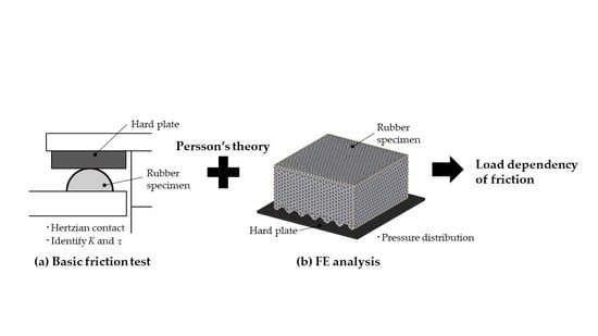
Based on the above, the procedure for predicting the friction force using FE analysis is as follows. Here, the basic friction test deals with the contact between the hemispherical rubber specimen and flat plate, where the contact form can be described by Hertz’s contact theory. Figure 1 shows a schematic of the proposed methodology for predicting rubber adhesive friction.
- (1)
- The basic friction test is carried out under several contact load conditions using the target rubber and hard plate specimens (Figure 1a).
- (2)
- The friction coefficient between the hemispherical rubber specimen and hard plate is given by:Here, it is confirmed that although the contact pressure distribution between the hemisphere and flat plate during sliding does not necessarily follow the pressure distribution of Hertz’s theory, the influence on the parameter determination due to the difference is small enough in the range of the examined conditions [15].
- (3)
- To identify parameters K and , the results of the friction test and Equation (9) are compared under several contact load conditions.
- (4)
- The frictional contact boundary value problem, which is the target phenomenon to predict the adhesive friction, is analyzed by the FE method. Although the target materials and the roughness of the rubber surface are the same as those of (1), any condition, such as the load condition and the contact form (for instance, the geometric pattern of the rubber surface), can be used (Figure 1b).
- (5)
- Acquire the pressure distribution at the microscopic apparent contact area evaluated with the element size or node distance as the representative length (Figure 1c).
- (6)
- Substitute the parameters K and already identified in (3) and the pressure distribution data obtained in (5) into Equation (8). Then, by integrating over the apparent contact area, the friction force can be evaluated taking the contact load dependency into account. Here, the pressure distribution is the sliding time at which the frictional force is desired to be evaluated. Further, if the time history data are available, the time series variation of the frictional force (or friction coefficient) can be predicted.
3. Results and Discussion
To verify the proposed method, we predicted the friction coefficient for the contact between a hemispherical PDMS (poly-dimethyl siloxane) specimen and a PMMA (polymethyl methacrylate) flat plate, and for the contact between a PDMS block specimen with a grooved surface and a prism flat plate. For details of the molding process of PDMS, refer to Maegawa et al. [15].
In this study, a commercial software package, MSC Marc, was used for FE analysis. We adopted a linear elastic body for the constitutive model of PDMS, while we assumed that the PMMA and prism are rigid bodies. The updated Lagrangian method was used for the treatment of geometric nonlinearity. Further, we adopted Amonton–Coulomb’s law based on the surface-to-surface contact discretization method.
3.1. Friction between Hemispherical Rubber and the Flat Plate
3.1.1. Basic Friction Test
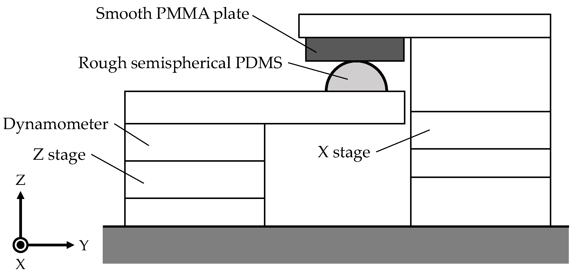
First, assume that the friction test [15] between the hemispherical PDMS rubber specimen with roughness and the smooth PMMA plate is targeted at predicting the friction coefficient. Figure 2 shows the schematic view of the friction test for a hemispherical PDMS rubber specimen and PMMA plate contact, where the radius of the hemispherical PDMS is 9.5 mm. The friction test was conducted under constant sliding velocity and constant normal load.
In the friction test, one of the authors prepared three types of hemispherical rubber specimens with the same compounding ratio, then different rough surfaces were created using different emery papers for each PDMS specimen. The surface roughness of the specimens were Specimen I (), Specimen II () and Specimen III (). The Young’s modulus was determined through the JKR contact test [17,18] as E = 1.2 MPa, whereas the Poisson’s ratio was set to [19]. In the friction test shown in Figure 2, Hertz contact can be assumed; thus, we identified the parameters K and using Equation (9). Table 1 presents the fitting results. Here, we assume that the shear strength depends only on the combination of materials. Therefore, we identified the constant value regardless of the surface roughness, whereas we identified three different values of K for each specimen.
3.1.2. FE Analysis and Prediction of Adhesive Friction
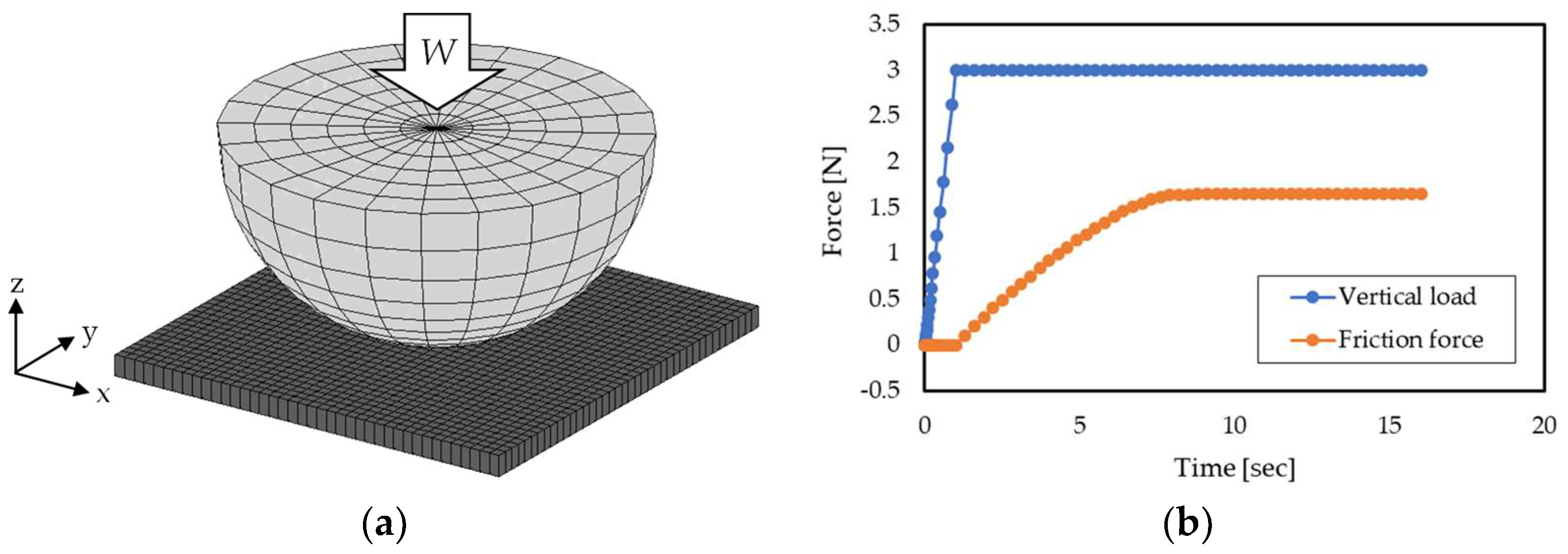
This section focuses on the same problem as considered in the basic friction test, for the prediction of adhesive friction. Figure 3 shows the FE analysis model and typical result of the contact forces. We adopted the eight-node solid element. To obtain a smooth contact pressure distribution, the contact part was discretized using fine elements. In the FE analysis, after applying a prescribed vertical load for the rigid shell element attached to the upper surface of the hemispherical PDMS, the rigid PMMA was allowed to move with a velocity of 0.1 mm/s in the x-direction and slid for 15 s.
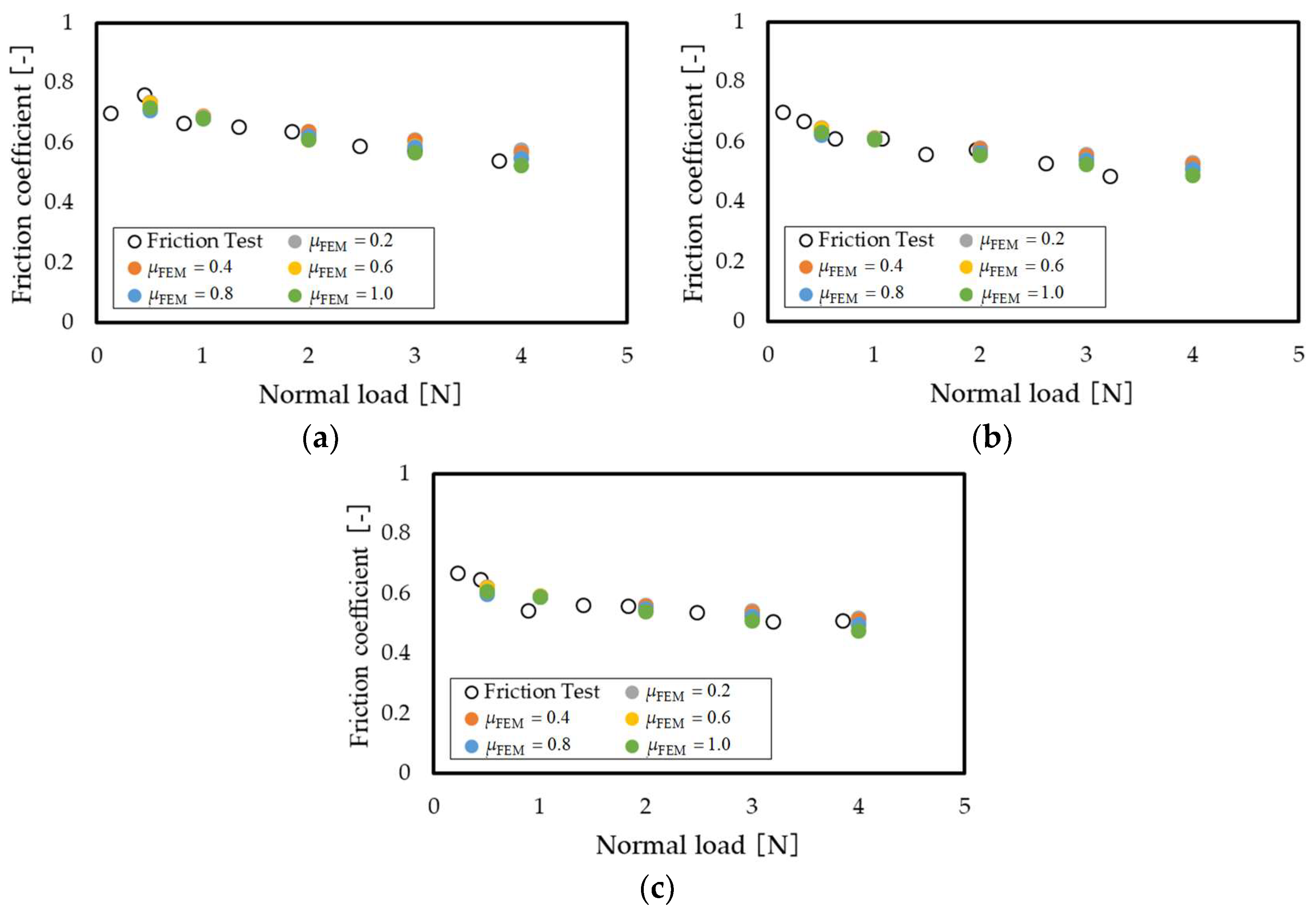
The friction coefficient itself is an input value in the FEM. However, it is considered that it does not exert a large influence on the pressure distribution if the magnitude of friction is within a certain range. To examine this point, we also carried out an analysis when the input value of the friction coefficient in FEM was set to 0.2, 0.4, 0.6, 0.8 and 1.0 for this prediction.
Figure 4 shows the contact load dependency of the friction coefficient predicted from the pressure distribution obtained by FE analysis and the already obtained K and . As can be observed in the figure, the predicted results and the test results are in good agreement. That is, it is possible to express the decrease of the friction coefficient as the load increases. In addition, we can predict the effect of the surface roughness on the contact load dependency of the friction coefficient. Furthermore, it can be confirmed that almost the same friction coefficient can be predicted regardless of the input value of the friction coefficient in the FEM. The effect of the friction coefficient on the contact pressure distribution obtained by FE analysis is small. Hence, it is considered that adhesive friction can be, to a certain extent, predicted by the proposed method in FE analysis by setting a practical value of .
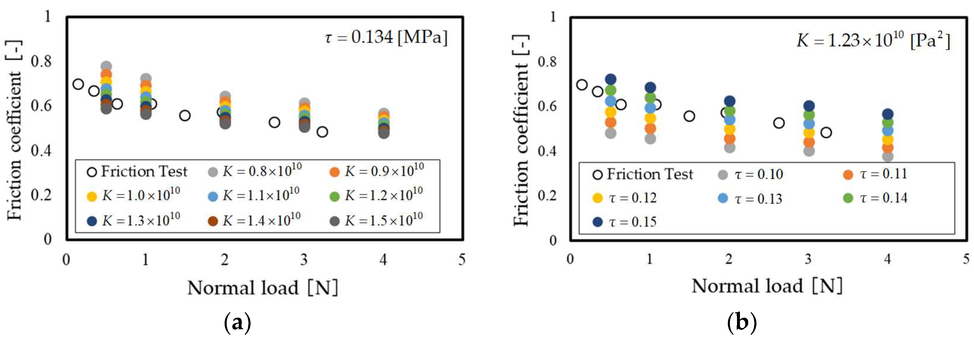
To examine the quality and the influence of fitting parameters K and , we conducted the sensitivity analysis, as shown in Figure 5. In the analysis, we set eight values of K and six values of referring to the fitting results shown in Table 1. The shear strength affects the magnitude of friction force, while the parameter K affects the gradient with respect to the load dependency of the friction force. From the results in Figure 4 and Figure 5, it is thought that the present fitting method and significant figures are reasonable. However, note that further investigation is necessary for the validity of K and its identification method.
3.2. Friction between the Rubber Block with a Grooved Surface and the Flat Plate
3.2.1. Basic Friction Test
Next, for the case with geometric patterns on the contact surface, we attempted to predict the adhesive friction between the rubber block specimen with a grooved surface and the flat plate. The materials for the rubber block specimen and the flat plate are PDMS and prism, respectively.
To identify the parameters K and , we molded the hemispherical PDMS, which has the same compounding ratio as the PDMS block, and then, each surface roughness was controlled at the same value using the emery paper. Then, we conducted the basic friction test using the apparatus shown in Figure 2, while the radius of the hemispherical PDMS specimen was 18 mm. Similarly, as presented in Section 3.1, we determined the Young’s modulus based on the JKR contact test [17,18] as E = 1.2 MPa, while the Poisson’s ratio was set to [19]. By comparing the results of the basic friction test between the hemispherical PDMS and prism plate for five levels of contact loads (0.45–6.69 N) with Equation (9), the parameters K and were identified as follows:
3.2.2. FE Analysis and Prediction of Adhesive Friction
Figure 6 shows the dimension of the PDMS blocks with a grooved surface, which are the targets for the prediction of adhesive friction. We prepared two types of specimens with a constant groove depth, but different pitch. Note that the surface roughness and compounding ratio were the same as those of the hemispherical PDMS specimen described in the basic friction test of Section 3.2.1.
Figure 7a shows the measurement system of the friction between the PDMS block with a grooved surface and the prism plate. The surface of the prism is smooth enough compared to the PDMS block. In the measurement of adhesive friction, the prism plate was pushed from a lower side against the PDMS block fixed to the upper jig, and the prism plate was then driven horizontally while keeping a constant pressing displacement. The normal and tangential forces during sliding were measured using a dynamometer. We measured the friction coefficient between the PDMS block with a grooved surface and the prism plate for five levels of pressing displacement.
Figure 7b shows the FE model corresponding to the contact between the PDMS block with a grooved surface and the prism plate. Here, we adopted the eight-node solid element. To obtain a smooth contact pressure distribution, the contact part was discretized using fine elements. In the FE analysis, the boundary condition corresponding to the measurement method was set. That is, after applying the prescribed vertical displacement to the rigid shell elements attached to the upper surface of the PDMS block with a grooved surface, the rigid prism was allowed to move with a horizontal sliding velocity of 1.0 mm/s in the x-direction. The sliding period was set to 10 s. In addition, the friction coefficient in the FE analysis was set to .
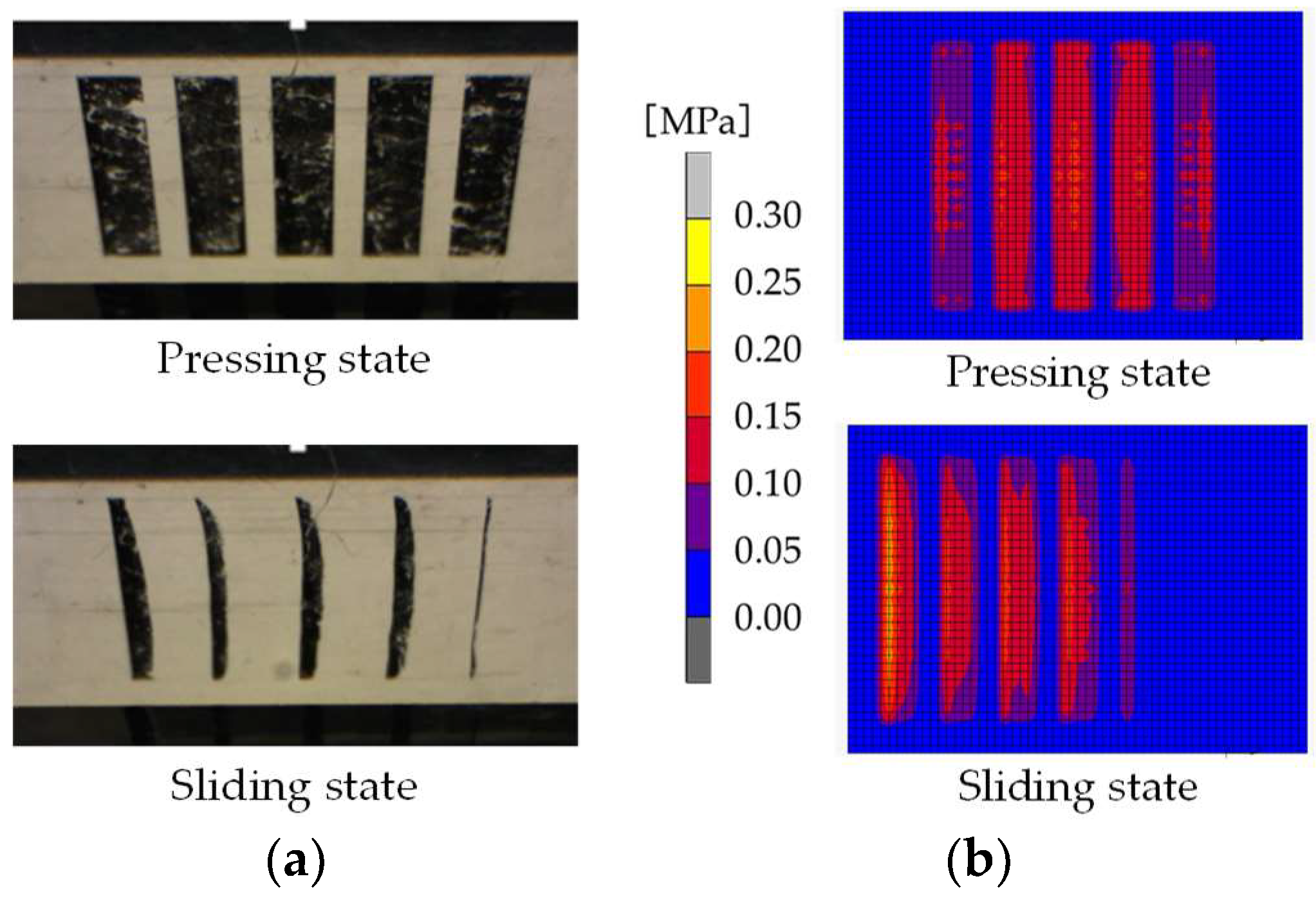
For the prediction of the friction coefficient, we adopted the distribution of the steady state value of the contact pressure. Figure 8a shows an example of the visualized distributions of the real contact in the experiment. Here, the dark region corresponds to the dense part of the real contact area. Further, Figure 8b shows an example of the contact pressure distributions obtained by FEM. These results were obtained using Specimen B at 0.8 mm of vertical displacement. It can be observed from the figure that there is a corresponding relationship between the real contact area obtained by experiment and the contact pressure distribution obtained by FE analysis.
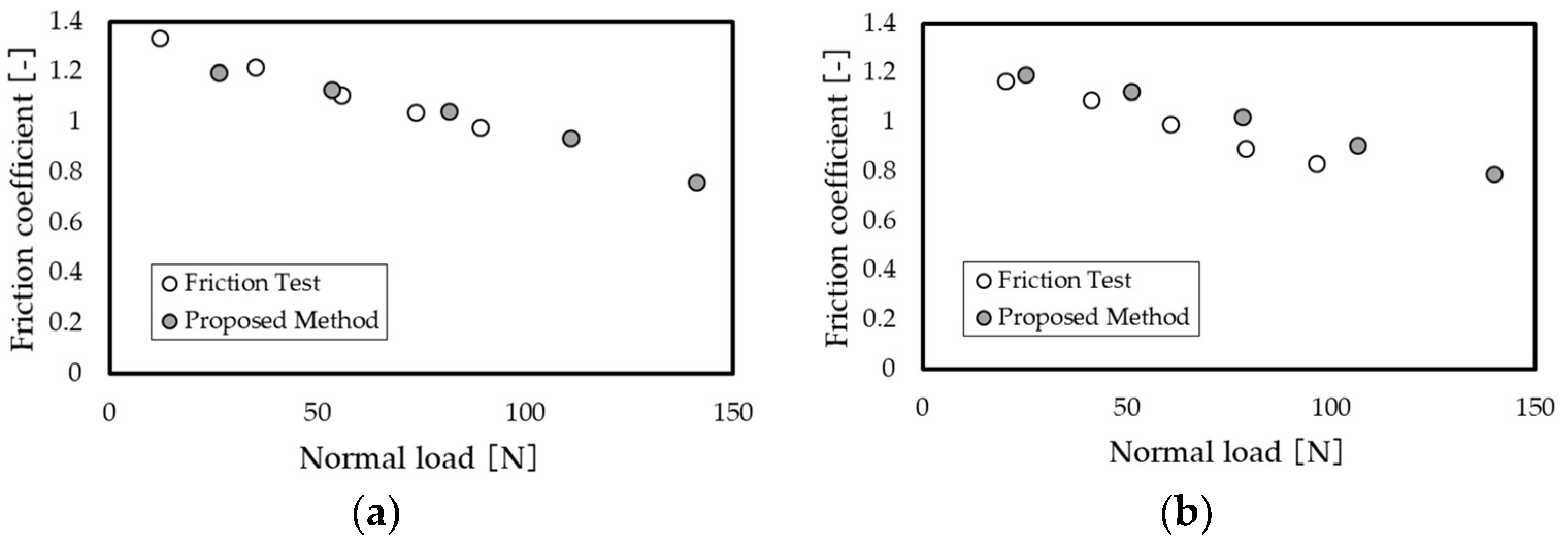
Figure 9 shows the contact load dependency of the friction coefficient predicted from the pressure distribution obtained by FE analysis and the K and values identified using Equation (10). The figure also includes the experimental results. As can be observed from the figure, the prediction results and the experimental results are in good agreement, and it is possible to express the decrease of the friction coefficient as the contact load increases. Furthermore, when the surface pattern of the rubber block is changed, the change in the friction can be predicted, if the target rubber specimens have the same material property and surface roughness. However, there was no perfect agreement with the experimental results, and the accuracy of the prediction result deteriorated especially for Specimen B. This is because when the contact surface has a complicated pattern, it is necessary to obtain an accurate pressure distribution. Thus, in such cases, the contact surface should be discretized more precisely using finer meshes. In addition, for the constitutive model, we adopted a linear elastic body, which cannot adequately describe the rubber deformation; this is another reason for the reduced prediction accuracy of the proposed method.
4. Conclusions
In this study, we proposed a method to predict rubber adhesive friction for an arbitrary contact type by combining the basic friction test, Persson’s contact theory and FE analysis. We prepared two types of specimens and measured the friction. Thereafter, the friction coefficient obtained by the proposed method was quantitatively compared with experimental result. It was confirmed that the prediction accuracy of the contact load dependency of the friction coefficient using the proposed method is reasonably good. Note that it is necessary to set the friction coefficient to a practical value to a certain extent. In particular, further investigation is required when the rubber significantly deforms due to friction. Besides, to identify the unknown parameters K and in the proposed method, we can directly use the profile of the contact pressure distribution obtained using FE analysis instead of Equation (9) when the contact type of the basic friction test does not obey the Hertz contact.
Moreover, the prediction accuracy of the proposed method could be improved by adopting a sophisticated discretization of the contact surface and an advanced constitutive model such as the hyper-elastic body for rubber, in the FE analysis. Note that since we focused on the fully sliding stage of the contact surface, the proposed method cannot deal with problems such as the Mindlin slip, in which the sticking and slipping regions coexist.
Acknowledgments
We would like to thank Editage (www.editage.jp) for English language editing.
Author Contributions
Keishi Mieda and Takeru Matsuura performed the FEA and evaluation of friction coefficient. Satoru Maegawa conducted the experiments and provided the associated detailed data. Shingo Ozaki proposed the method and wrote the paper.
Conflicts of Interest
The authors declare no conflicts of interest.
References
- Tabor, D. Hysteresis losses in the friction of lubricated rubber. Rubber Chem. Technol. 1960, 33, 142–150. [Google Scholar] [CrossRef]
- Roberts, A.D. A guide to estimating the friction of rubber. Rubber Chem. Technol. 1992, 65, 673–686. [Google Scholar] [CrossRef]
- Fuller, K.N.G.; Tabor, D. The effect of surface roughness on the adhesion of elastic solids. Proc. R. Soc. Lond. A 1975, 345, 327–342. [Google Scholar] [CrossRef]
- Persson, B.N.J. Theory of rubber friction and contact mechanics. J. Chem. Phys. 2001, 115, 3840–3861. [Google Scholar] [CrossRef]
- Roberts, A.D.; Thomas, A.G. The adhesion and friction of smooth surfaces. Wear 1975, 33, 45–64. [Google Scholar] [CrossRef]
- Persson, B.N.J.; Volokitin, A.I. Rubber friction on smooth surfaces. Eur. Phys. J. E 2006, 21, 69–80. [Google Scholar] [CrossRef] [PubMed]
- Greenwood, J.A.; Williamson, J.B.P. Contact of nominally flat surfaces. Proc. R. Soc. Lond. A 1966, 295, 300–319. [Google Scholar] [CrossRef]
- Johnson, K.L. Contact Mechanics; Cambridge University Press: Cambridge, UK, 2003; ISBN 978-0521347969. [Google Scholar]
- Yang, C.; Tartaglino, U.; Persson, B.N.J. A multiscale molecular dynamics approach to contact mechanics. Eur. Phys. J. E 2006, 19, 47–58. [Google Scholar] [CrossRef] [PubMed]
- Johnson, K.L.; Greenwood, J.A.; Higginson, J.G. The contact of elastic regular wavy surfaces. Int. J. Mech. Sci. 1985, 27, 383–396. [Google Scholar] [CrossRef]
- Manners, W. Pressure required to flatten an elastic random rough profile. Int. J. Mech. Sci. 2000, 42, 2321–2336. [Google Scholar] [CrossRef]
- Hyun, S.; Pei, L.; Molinari, J.-F.; Robbins, M.O. Finite-element analysis of contact between elastic self-affine surfaces. Phys. Rev. E 2004, 70, 026117. [Google Scholar] [CrossRef] [PubMed]
- Persson, B.N.J.; Bucher, F.; Chiaia, B. Elastic contact between randomly rough surfaces: Comparison of theory with numerical results. Phys. Rev. B 2002, 65, 184106. [Google Scholar] [CrossRef]
- Yang, C.; Persson, B.N.J. Contact mechanics: Contact area and interfacial separation from small contact to full contact. J. Phys. Condens. Matter 2008, 20, 215214. [Google Scholar] [CrossRef]
- Maegawa, S.; Itoigawa, F.; Nakamura, T. Effect of normal load on friction coefficient for sliding contact between rough rubber surface and rigid smooth plane. Tribol. Int. 2015, 92, 335–343. [Google Scholar] [CrossRef]
- Persson, B.N.J. On the fractal dimension of rough surfaces. Tribol. Lett. 2014, 54, 99–106. [Google Scholar] [CrossRef]
- Johnson, K.L.; Kendall, K.; Roberts, A.D. Surface energy and the contact of elastic solids. Proc. R. Soc. Lond. A 1971, 324, 301–313. [Google Scholar] [CrossRef]
- Maegawa, S.; Nakano, K. Dynamic behavior of contact surfaces in the sliding friction of a soft material. J. Adv. Mech. Des. Syst. 2007, 1, 553–561. [Google Scholar] [CrossRef]
- Mark, J.E. (Ed.) Polymer Data Handbook; Oxford University Press: Oxford, UK, 1999; ISBN 978-0195181012. [Google Scholar]
Figure 1.
Proposed methodology for predicting rubber adhesive friction: (a) basic friction test; (b) an example of the FE analysis model for arbitrary target problems; (c) an example of the pressure distribution obtained by FE analysis.
Figure 1.
Proposed methodology for predicting rubber adhesive friction: (a) basic friction test; (b) an example of the FE analysis model for arbitrary target problems; (c) an example of the pressure distribution obtained by FE analysis.
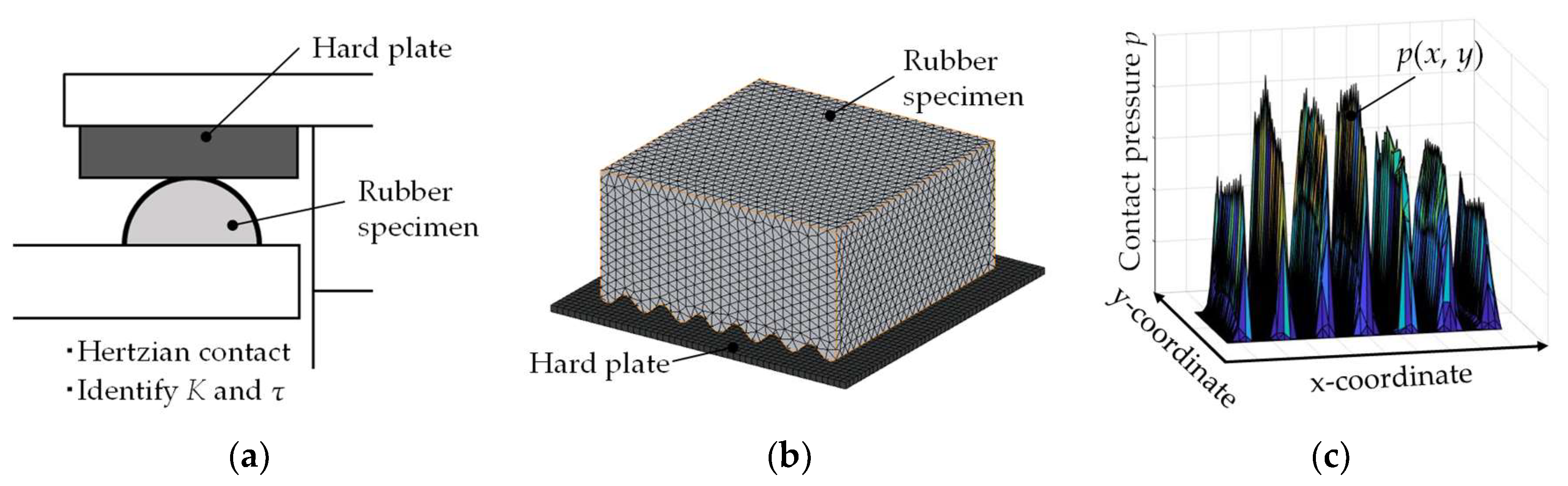
Figure 2.
Schematic view of the basic friction test between a hemispherical PDMS specimen and PDMS plate. The friction test was conducted under constant sliding velocity and constant normal load. The radius of the hemispherical PDMS specimen is 9.5 mm.
Figure 2.
Schematic view of the basic friction test between a hemispherical PDMS specimen and PDMS plate. The friction test was conducted under constant sliding velocity and constant normal load. The radius of the hemispherical PDMS specimen is 9.5 mm.

Figure 3.
FE analysis: (a) FE model of the hemispherical PDMS specimen and PMMA plate contact for obtaining the contact pressure distribution during sliding. The boundary condition was prescribed referring to the friction test, i.e., the same constant sliding velocity and constant normal load were set. (b) Result of contact forces under the condition of normal load of 3 N and friction coefficient .

Figure 4.
Variation of the friction coefficient with contact load obtained using the friction test and the proposed method: (a) Specimen I; (b) Specimen II; and (c) Specimen III. Although the results of the proposed method were obtained for various levels of , the effect of is minimal.
Figure 4.
Variation of the friction coefficient with contact load obtained using the friction test and the proposed method: (a) Specimen I; (b) Specimen II; and (c) Specimen III. Although the results of the proposed method were obtained for various levels of , the effect of is minimal.

Figure 5.
Example of the sensitivity of fitting parameters K and in the case of Specimen II: (a) effect of K; (b) effect of .
Figure 5.
Example of the sensitivity of fitting parameters K and in the case of Specimen II: (a) effect of K; (b) effect of .

Figure 6.
Dimensions of PDMS block specimens with a grooved surface (unit: mm): (a) Specimen A; (b) Specimen B.
Figure 6.
Dimensions of PDMS block specimens with a grooved surface (unit: mm): (a) Specimen A; (b) Specimen B.
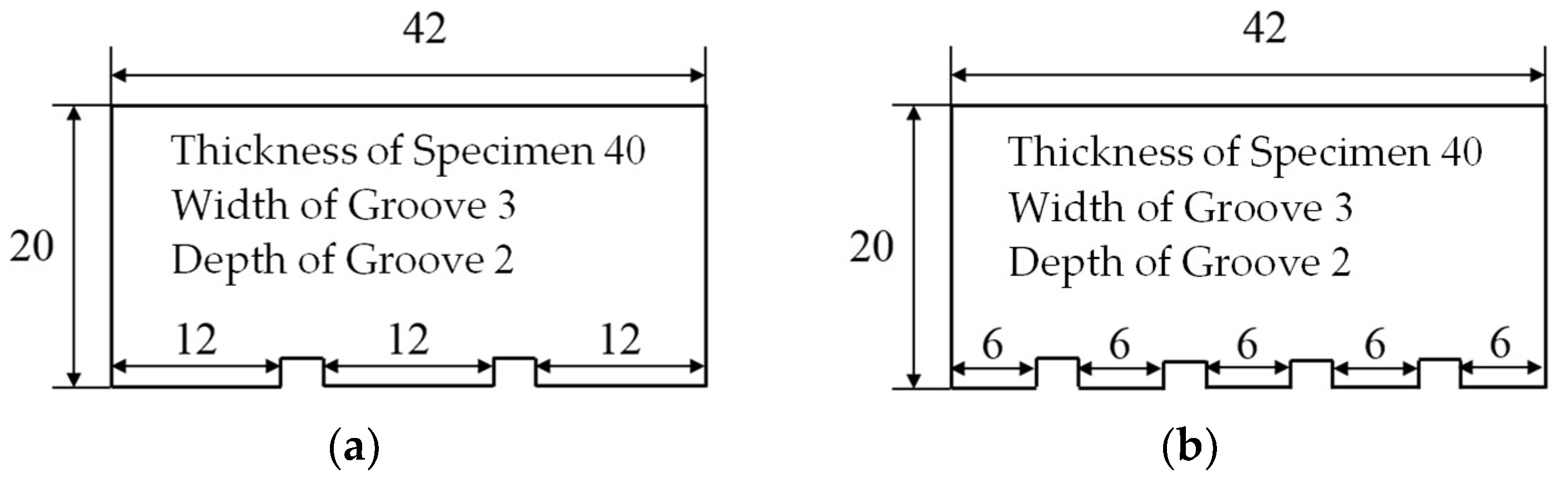
Figure 7.
Contact between the PDMS block specimen with a grooved surface and the prism plate: (a) measurement system and specimen; (b) FE model for Specimen A.
Figure 7.
Contact between the PDMS block specimen with a grooved surface and the prism plate: (a) measurement system and specimen; (b) FE model for Specimen A.
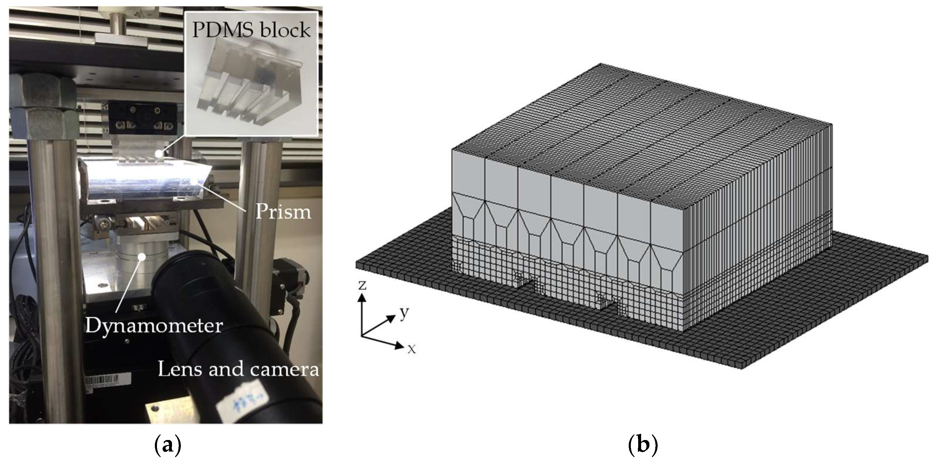
Figure 8.
Correlation between the results obtained by experiment and FE analysis: (a) visualized distribution of real contact area in the experiment; (b) pressure distribution obtained by FE analysis. These results were obtained using Specimen B with a pressing displacement of 0.8 mm.
Figure 8.
Correlation between the results obtained by experiment and FE analysis: (a) visualized distribution of real contact area in the experiment; (b) pressure distribution obtained by FE analysis. These results were obtained using Specimen B with a pressing displacement of 0.8 mm.

Figure 9.
Variation of the friction coefficient with the contact load obtained by the experiment and proposed method: (a) Specimen A; (b) Specimen B. The larger contact load corresponds to a larger pressing displacement. The results of the proposed method were obtained considering .
Figure 9.
Variation of the friction coefficient with the contact load obtained by the experiment and proposed method: (a) Specimen A; (b) Specimen B. The larger contact load corresponds to a larger pressing displacement. The results of the proposed method were obtained considering .

Table 1.
Fitting results of the characteristic value K for each surface roughness and shear strength .
Table 1.
Fitting results of the characteristic value K for each surface roughness and shear strength .
| Specimen I | Specimen II | Specimen III |
|---|---|---|
© 2018 by the authors. Licensee MDPI, Basel, Switzerland. This article is an open access article distributed under the terms and conditions of the Creative Commons Attribution (CC BY) license (http://creativecommons.org/licenses/by/4.0/).
Share and Cite
MDPI and ACS Style
Ozaki, S.; Mieda, K.; Matsuura, T.; Maegawa, S. Simple Prediction Method for Rubber Adhesive Friction by the Combining Friction Test and FE Analysis. Lubricants 2018, 6, 38. https://doi.org/10.3390/lubricants6020038
AMA Style
Ozaki S, Mieda K, Matsuura T, Maegawa S. Simple Prediction Method for Rubber Adhesive Friction by the Combining Friction Test and FE Analysis. Lubricants. 2018; 6(2):38. https://doi.org/10.3390/lubricants6020038
Chicago/Turabian StyleOzaki, Shingo, Keishi Mieda, Takeru Matsuura, and Satoru Maegawa. 2018. "Simple Prediction Method for Rubber Adhesive Friction by the Combining Friction Test and FE Analysis" Lubricants 6, no. 2: 38. https://doi.org/10.3390/lubricants6020038
Note that from the first issue of 2016, this journal uses article numbers instead of page numbers. See further details here.