Dynamical Simulations of a Flexible Rotor in Cylindrical Uncavitated and Cavitated Lubricated Journal Bearings


1
Department of Industrial Engineering, University of Salerno, 84084 Salerno, Italy
2
Department of Mechanical Engineering, Chemical and Industrial Design, Universidad Politécnica de Madrid (UPM), 28012 Madrid, Spain
3
Mechanical Engineering Faculty in Slavonski Brod, J. J. Strossmayer University of Osijek, HR-35000 Slavonski Brod, Croatia
*
Author to whom correspondence should be addressed.
Lubricants 2018, 6(2), 40; https://doi.org/10.3390/lubricants6020040
Submission received: 5 February 2018
/
Revised: 16 April 2018
/
Accepted: 20 April 2018
/
Published: 25 April 2018
(This article belongs to the Special Issue Tribology of Machine Elements--Smart Lubricants)
Abstract
:Due to requirements of their operating conditions, such as high speed, high flexibility and high efficiency, rotating machines are designed to obtain larger operating ranges. These operating conditions can increase the risk of fluid-induced instability. In fact, the presence of non-linear fluid forces when the threshold speed is overcome by the rotational speed, can generate rotor lateral self-excited vibrations known as “oil whirl” or “oil whip”. These instabilities derive from the interaction between the rotor and the sliding bearing and they are typically sub-synchronous and they contribute to eventual rubbing between rotor and stator with consequent damage to the rotating machines. For these reasons, the aim of this paper is to numerically investigate the differences in the dynamic behaviour of a flexible rotor supported by cylindrical lubricated journal bearings. The study considers two different cases, uncavitated and cavitated lubricated films, in order to develop an original Matlab-Simulink algorithm for the numerical solution of the differential non-linear equations of motion of the unbalanced flexible rotor supported on hydrodynamic journal bearings. The bearings were modelled as uncavitated and cavitated (π-Film) short bearings derived from classical Reynolds’ theory. Dynamic simulation allowed prediction of the shape and size of the orbit performed by the system and evaluation of the vibrating phenomena exerted by the rotor during the motion. The results show that cavitation completely modifies the behaviour of the system in every aspect. The analysis of the diagrams obtained showed that the proposed algorithm provides consistent results and represents a valuable instrument for dynamic analysis of rotating systems.
1. Introduction
Hydrodynamic journal bearings are extensively used to support rotors in turbomachinery. They can ensure low wear rate and high load-carrying capacity in a wide range of applications [1]. The coupled analysis of the rotor and journal bearing is of fundamental importance in the case of a flexible rotor in order to guarantee reliable operation of these dynamic systems. From a dynamical point of view, it is well known that a special type of self-excited vibrations may occur in the rotors mounted on journal bearings due to fluid dynamic phenomena in the oil film [2]. Instability phenomena due to the interaction between the rotating system and the oil film of the journal bearing are known as oil whirl and oil whip. They are characterized by sub-synchronous precessional motions [3,4]. In the presence of the oil whirl phenomenon, the whirl frequency increases with rotational speed, and it is typically around half the rotational speed. The residual unbalance give rise to a synchronous motion to which the whirl frequency is superimposed. Instability due to oil whip phenomena occurs when the sub-synchronous whirl frequency reaches the natural frequency of the elastic rotor system [5]. Oil whip instability is typically characterized by high vibration amplitudes. For this reason, this instability requires careful analysis in order to prevent excessive wear or even failure of the dynamical system. Typically, these instabilities are due to the forces of the oil film [6] and can be analysed in terms of stiffness and damping coefficients of the rotating system. In the last few years, research has demonstrated that the oil whirl occurs when the journal bearing operates with micropolar lubricant [6,7,8,9,10]. For this reason, the effect of the contamination of the lubricants [11] and of non-linear behaviour of film-oil journal bearings in rotating machines have been studied by many authors [12]. Harika et al. investigated the effect of water contamination of lubricants on hydrodynamic lubrication and the results show that the viscosity of the lubricant is modified by the presence of water in the lubricating oil. The same occurs for the thermal properties of the lubricant. In fact, the viscosity increase leads to an increase in the film thickness that can generate instability of the bearing under these operating conditions [13]. In addition, the bearing performance, in order to avoid instability phenomena, has been analysed, studied and simulated by considering factors such as misalignment [10], elasticity of the bearing liner [14], dynamic conditions and surface roughness [15,16]. Pennacchi et al. presented a study on the nonlinear effects caused by coupling misalignment in rotors equipped with journal bearings. The results of their simulations showed the presence of nonlinear effects in the system response [17]. Lund and Sternlicht [18] mathematically described a flexible rotor on fluid film bearing by coupling the dynamic characteristics of the bearing with the elastic characteristics of the rotor. They introduced the linearization of bearing forces predicted by the Reynolds equation, around its static equilibrium condition. This method has mostly been used for stability calculations. Subsequently, thanks to more powerful calculation systems and more precise simulation algorithms, it became possible to analyse different phenomena [19,20], such as: cavitation effects [21], thermal effects, shaft tilting effects and fluid inertia effects [22,23]. The behaviour of a dynamic system is mainly mathematically analysed by the representation in the state space and the formalism of the frequency domain. Van der Pol et al. verified empirically that the response of a system depends on the frequency of the driving force and that the same system can reveal different sub-harmonic motions depending on the initial conditions imposed [24]. This phenomenon is an important feature of non-linear systems. They also observed that if two dynamic systems have very similar initial conditions, the initial transient can also apparently be the same, but the final motion is completely different. Obviously, if the initial conditions of the two systems are the same, then the deterministic nature of equations ensures that the motion is identical for all of the time. However, uncertainty on the initial conditions is inevitable due to the physical nature of the systems; therefore, divergence of the motions cannot be avoided in the chaotic regime. This phenomenon is evident in the phase diagram.
The studies conducted by Van der Pol led to the conclusion that a combination of random events is very common in non-linear dynamics. Lorenz continued these studies and with the introduction of the concept of chaotic attractors, he built the first example of chaotic dynamics. In fact, the analysis of the power spectrum is an excellent instrument for identifying the attractors in the phase space. If the spectrum is continuous, then there is a chaotic attractor; if it is discrete, it denotes the absence of chaos [25]. The aim of this paper is to numerically investigate the differences in the dynamic behaviour of a flexible rotor supported by cylindrical lubricated journal bearings. The simulation was carried out by developing a new Matlab-Simulink algorithm for the numerical solution of the differential non-linear equations of motions of the unbalanced flexible rotor supported on hydrodynamic journal bearings. The bearings were modelled by using the Reynolds’ theory and adopting the models of Uncavitated and Cavitated (π-Film) Short Bearings. For the simulation, five real dynamic cases for the rotor bearing system were used.
2. Materials and Methods
2.1. The System
The analysed system consists of a hard disk spliced in the centreline of a flexible shaft. The disc has mass 2 m (Figure 1). The shaft is a thin bar of circular cross section and it has negligible mass compared to that of the disc. With these assumptions, the mass and the inertia contribution are exclusively from the disc. The flexibility originates exclusively from the shaft.
The disc is stiff and thin. It also remains perpendicular to the axis of rotation during the motion, thus the gyroscopic effect is negligible. The disc is also provided with a static imbalance, whereby the geometric centre does not coincide with the centre of mass.
The bearings are represented by cylindrical elements placed at the ends of the shaft and have the same characteristics.
Finally, it is possible to affirm that:
- the system is completely symmetrical with respect to the disc
- the motion of the disk is plane.
2.2. Journal Bearings
Under classical hypotheses of fluid-dynamic isoviscous lubrication, the Reynold’s equation, for the lubricated dynamical system under investigation, can be written in cylindrical coordinates [26] (Figure 2):
It is well known that under the hypothesis of a short bearing, it is possible to obtain a simplification of Reynold’s equation, for approaching simple analytical fluid film force expressions, which are useful in many rotor dynamic design problems.
In order to analyse and simulate the real behaviour of a flexible rotating dynamic system, the effects due to the cavitation (π-Film) of the lubricating fluid film must be taken into account [26].
The effects due to the cavitation of the fluid film add up to the force exerted on the journal by the bearing. The latter is calculated by integrating the pressure over the entire surface. The supply pressure and the eccentricity determine the extent of cavitation.
For this reason, in this paper two different configurations of the rotating system will be analysed, the uncavitated short bearing and the cavitated (π-Film) short bearing.
The two components of the fluid film force derive from a solution of the integrals, by setting the appropriate values of θ1 and θ2 according to the uncavitated and cavitated models:
Under this hypothesis the two force component for both cases are [26]:
Uncavitated Short Bearing
Cavitated (π-Film) Short Bearing
The expression in polar coordinates (ε, ψ) is very compact, but it is convenient, in order to define the equation of motion in a Cartesian system as shown in Figure 2, in which the centre of the coordinates is the centre of the bearing.
The coordinate transformation is given by [26]:
where the x and y represent the coordinates of the centre of the journal. The fluid film force will be not linearized because the analysis is desired for large motion.
2.3. Equations of Motion
The scalar equations of motion of the rotor-bearing system can be written as follows [26]:
in which Equations (10) and (11) have been obtained by imposing the dynamic balance of the centre of the disc C. Equations (12) and (13) have been derived from the dynamic balance of the centre of the Journal J.
The forces acting on the centre of the disc are:
- force of inertia
- spring force (k is the flexural stiffness of the shaft)
- centrifugal force of inertia
- static load (due to the rotor weight).
The forces acting on the centre of the journal are:
- nonlinear fluid film force
- spring force.
Since the shaft is massless, no inertia force acts on the centre of the journal. The system consists of four equations and four unknowns,. The unknowns are the coordinates of the journal centre and of the disc centre.
2.4. Numerical Integration of the Equations of Motion
With the aim of obtaining a numerical solution for the dynamic system of Equations (10)–(13), in this study an original algorithm was developed in the Matlab®-Simulink environment. Figure 3 shows as example the global Simulink scheme in the case of an uncavitated bearing.
Each part of the scheme corresponds to an equation from the system of Equations (10)–(13). In Figure 4, it is possible to observe the top of Figure 3 corresponding to Equation (10) in detail.
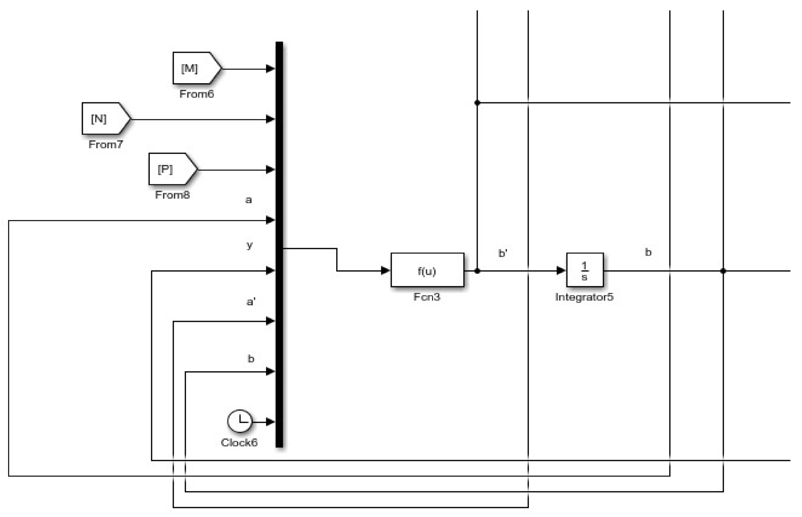
In Figure 5, it is possible to observe the bottom of Figure 3 corresponding to Equation (13) in detail.
The “auxiliary variables” were built in order to simplify the non-linear equations. These auxiliary variables are time-varying functions. In fact, they contain the coordinates of the centre of the journal. In the case of the uncavitated short bearing, the auxiliary variables that appear in Figure 3 and Figure 5, are:
The Simulink scheme for the Cavitated (π-Film) Short Bearing model is similar, but it was necessary to implement more auxiliary variables because of the greater mathematical complexity of this model. In this case the auxiliary variables, shown below, are:
For the simulation, five real dynamic cases for the rotor bearing system were used. Table 1 shows the values of the parameters related to the Uncavitated Short Bearing and Cavitated (π-Film) Short Bearing.
The simulations results were analysed by a displacements diagram; orbits in the x–y plane; the power spectrum; and phase diagrams.
3. Results and Discussions
3.1. Simulation 1
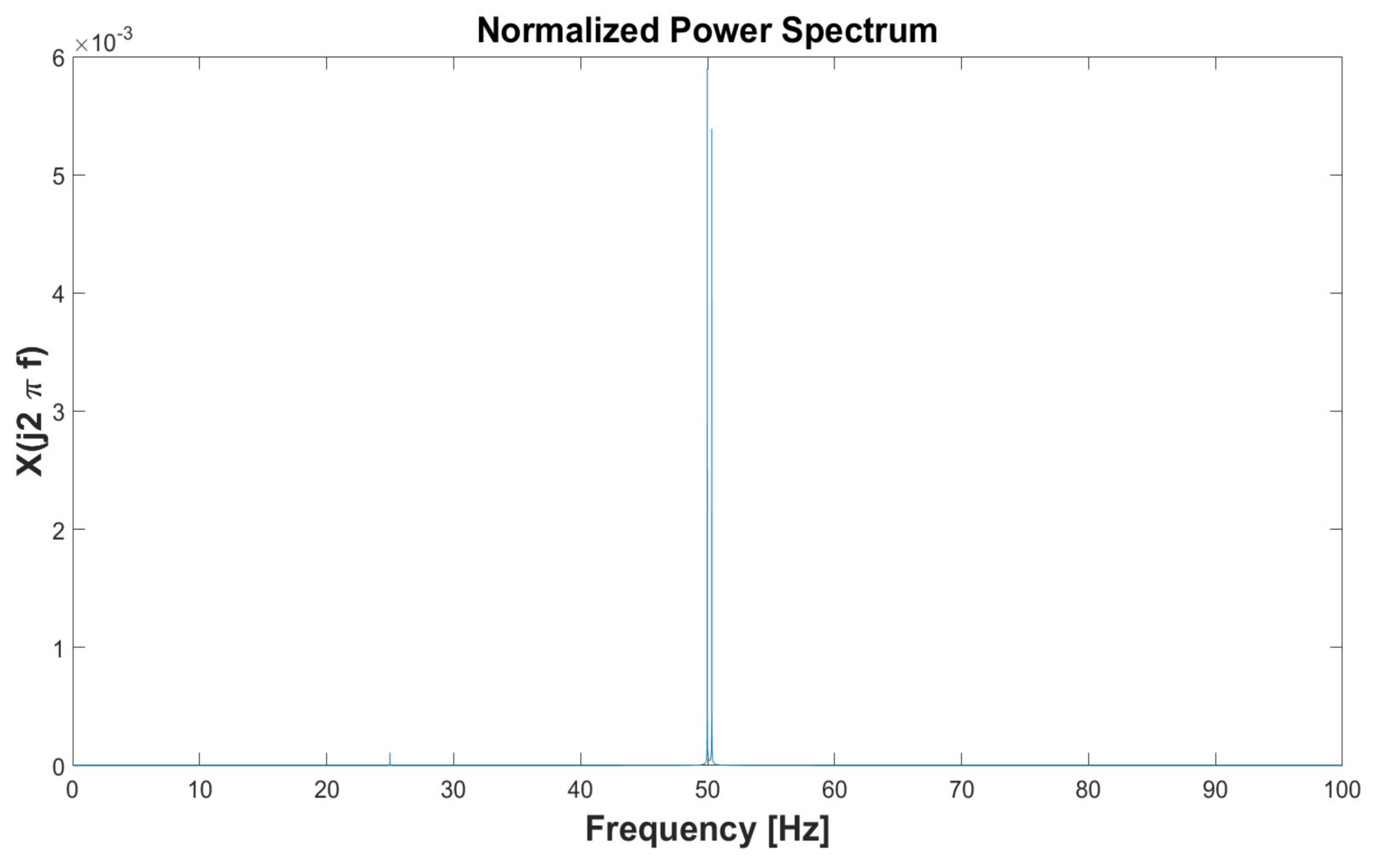
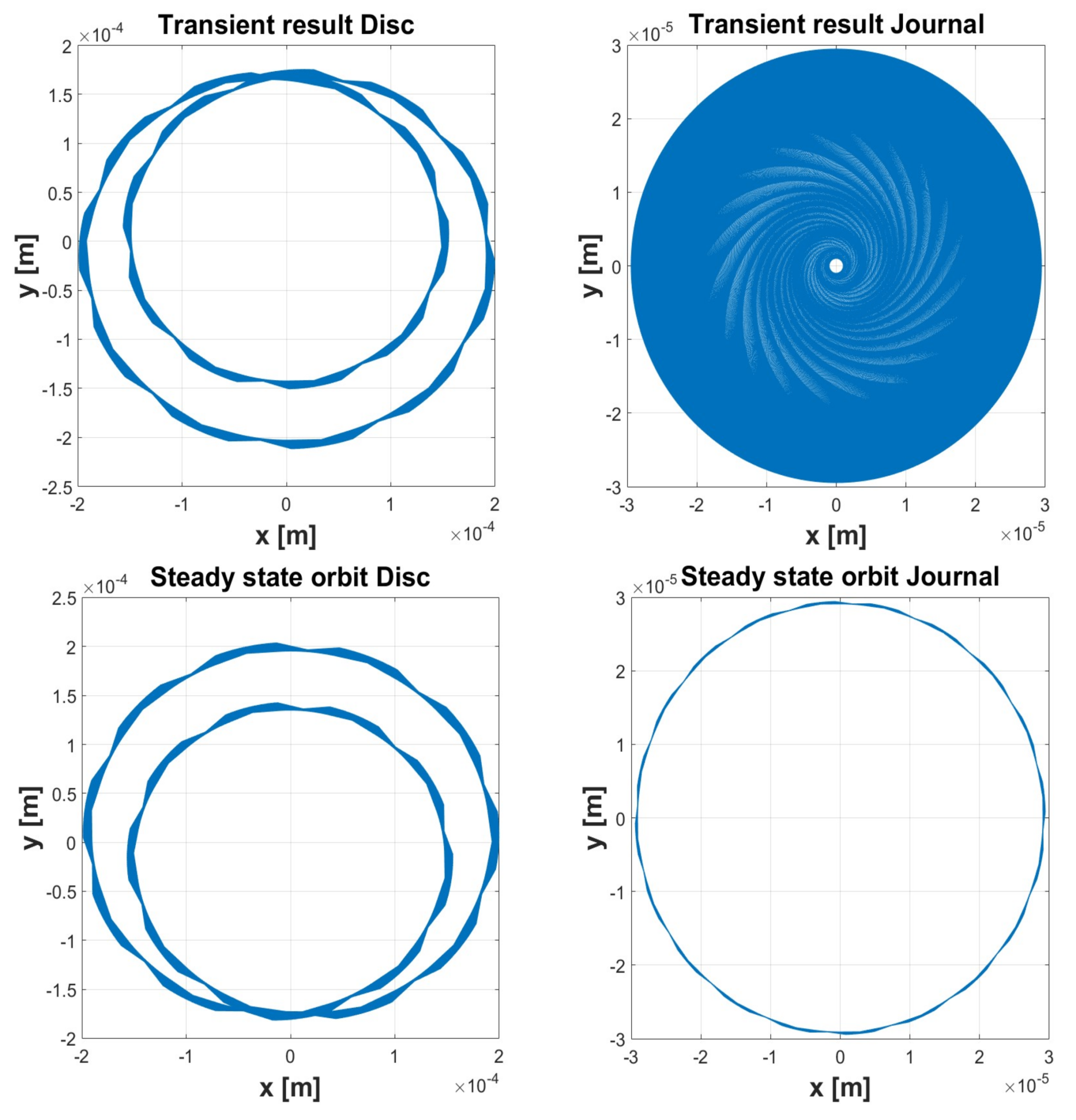
This simulation is characterized by flexural resonance because the angular speed of the rotor coincides with the natural frequency of the rotor-bearing system. In this case, it is possible to understand the dynamics of the rotor system by analysing the orbits in space. In the case of the uncavitated short bearing, the orbit of the disc centre increases steadily generating a concentric spiral until it reaches a stable condition. The steady orbit has a radius of 3 m. This is obviously not acceptable because the system will fault before reaching this condition. The steady orbit of the journal centre is a circle with a radius value very close to the radial clearance (Figure 6). The discrete power spectrum (Figure 7) indicates the absence of chaos and that the only significant vibration is at 50 Hz (frequency of the rotor).
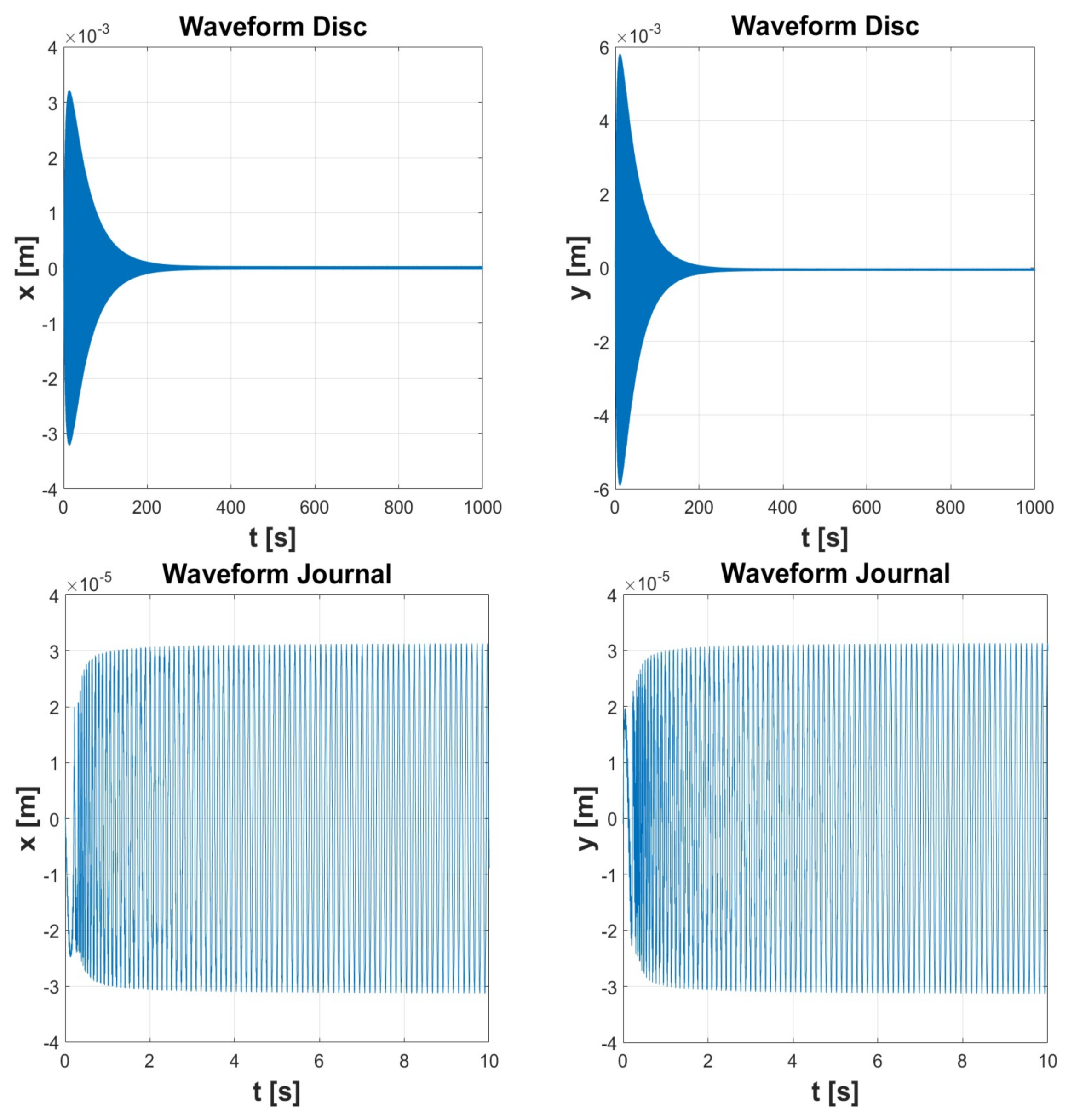
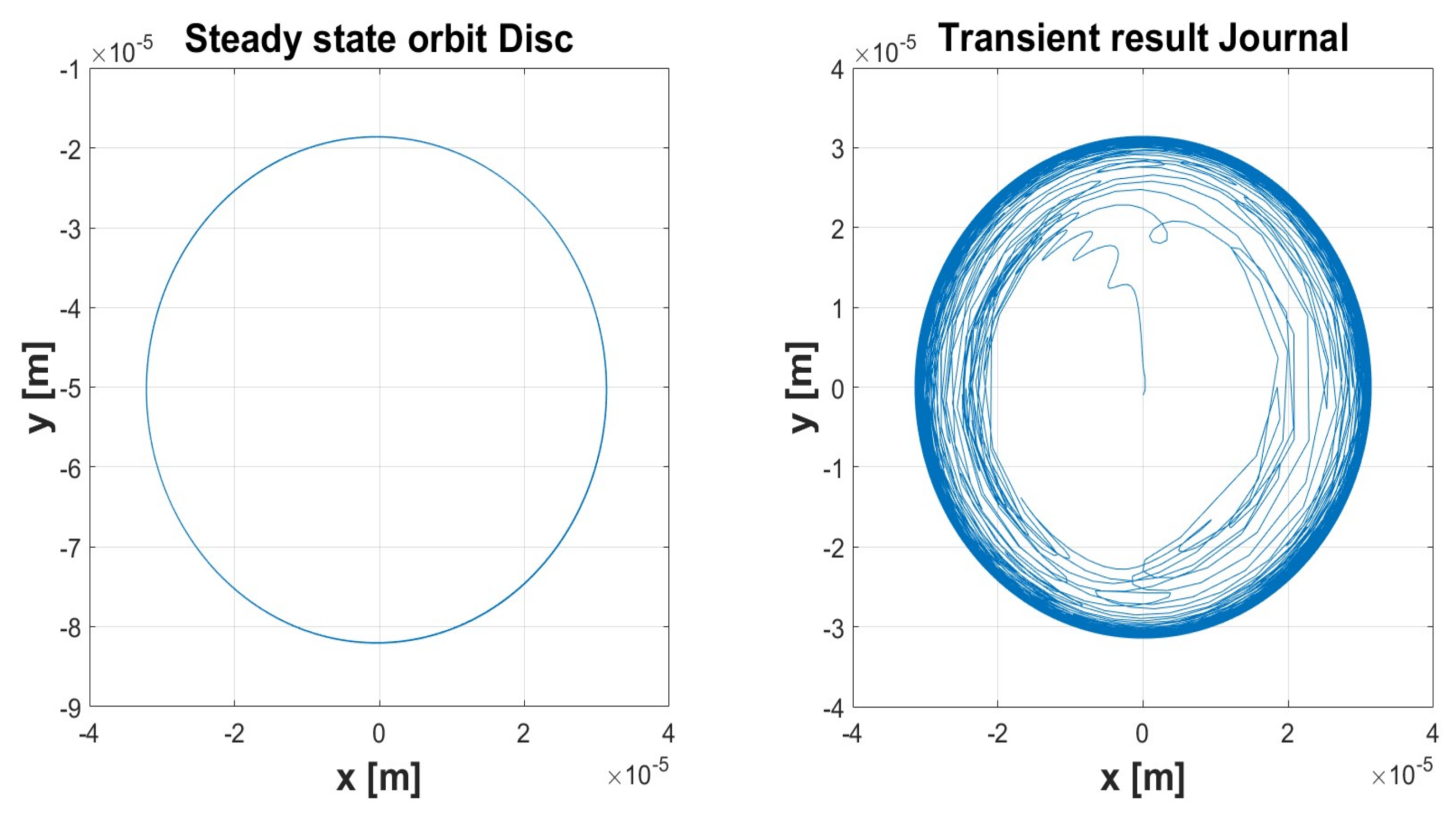
In the case of the cavitated short bearing, the model also returns a periodic manner for the disc centre. The maximum amplitude of this orbit is smaller than the uncavitated bearing. The transient of the journal centre is different but the steady orbit is the same (Figure 8). The power spectrum is almost the same (Figure 9).
3.2. Simulation 2
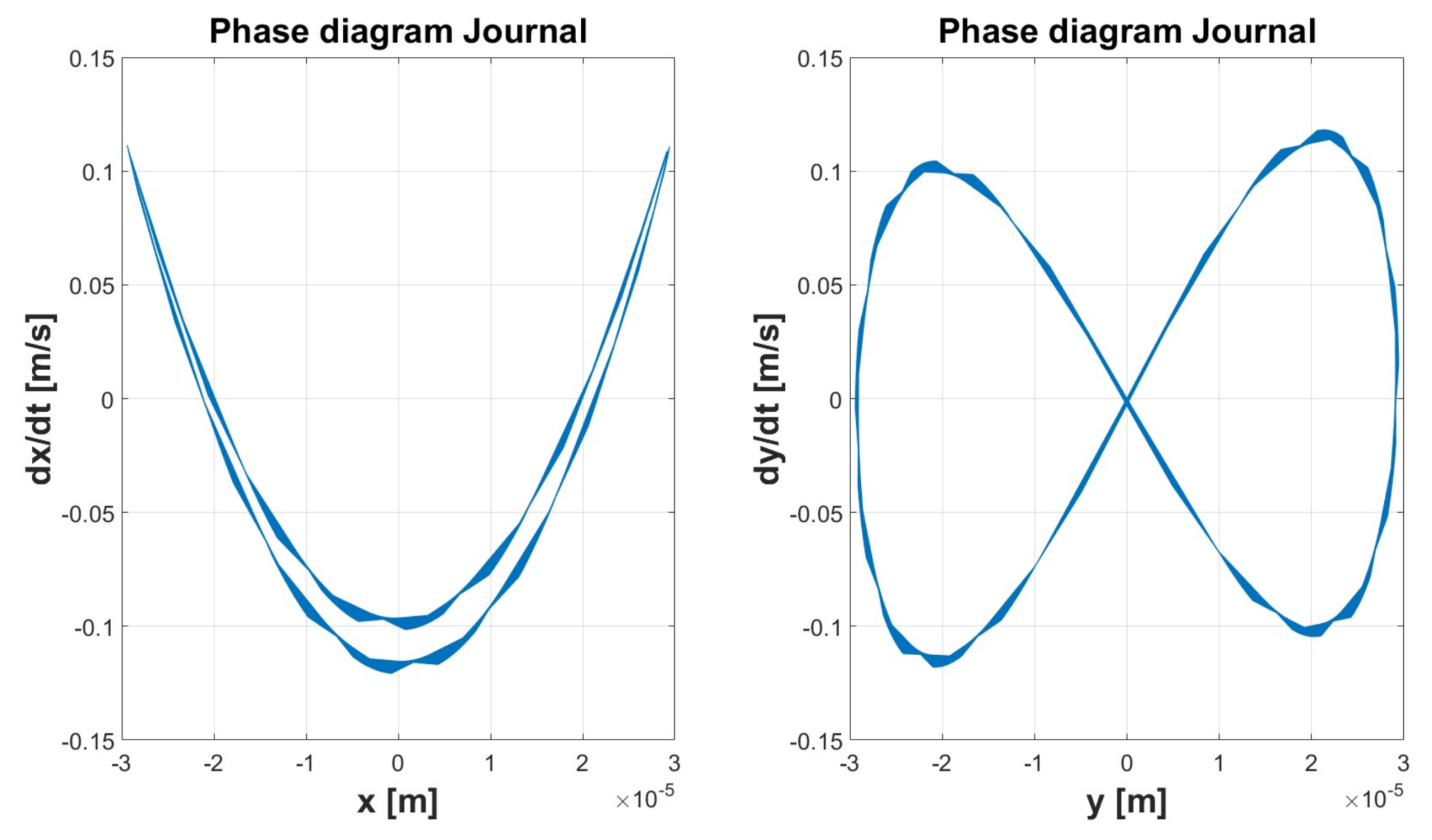
In this section are presented the results for the simulation 2 (Table 1) for the uncavitated short bearing (Figure 10, Figure 11 and Figure 12) and cavitated short bearing (Figure 13, Figure 14 and Figure 15). In this simulation the orbit assumes a particular shape during both the transition phase and during the steady phase reaching a stable operating condition. This can be observed in the phase diagrams, which show well-defined limit cycles (Figure 11 and Figure 14).
In the case of the uncavitated short bearing, the orbit of the centre of the disc increases during the initial transient but subsequently decreases, maintaining a shape with extra-loops. The steady orbit of the journal centre is a circle with a radius value very close to the radial clearance (Figure 10). The power spectrum (Figure 12) shows how the most relevant frequency is approximately 260 Hz. It is possible that this is asynchronous whirling because the natural frequency of the system is 259.9 Hz.
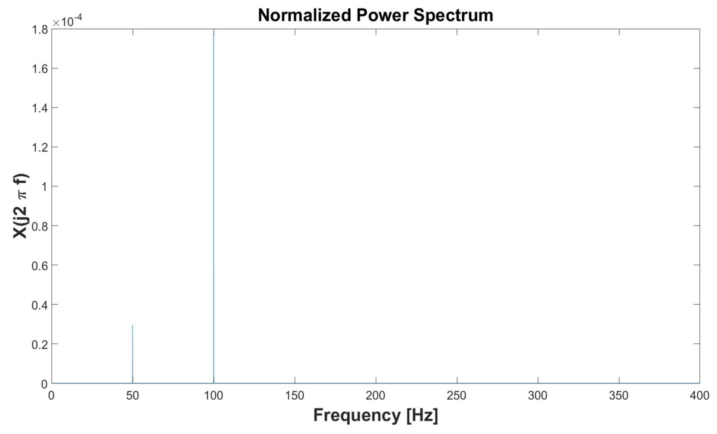
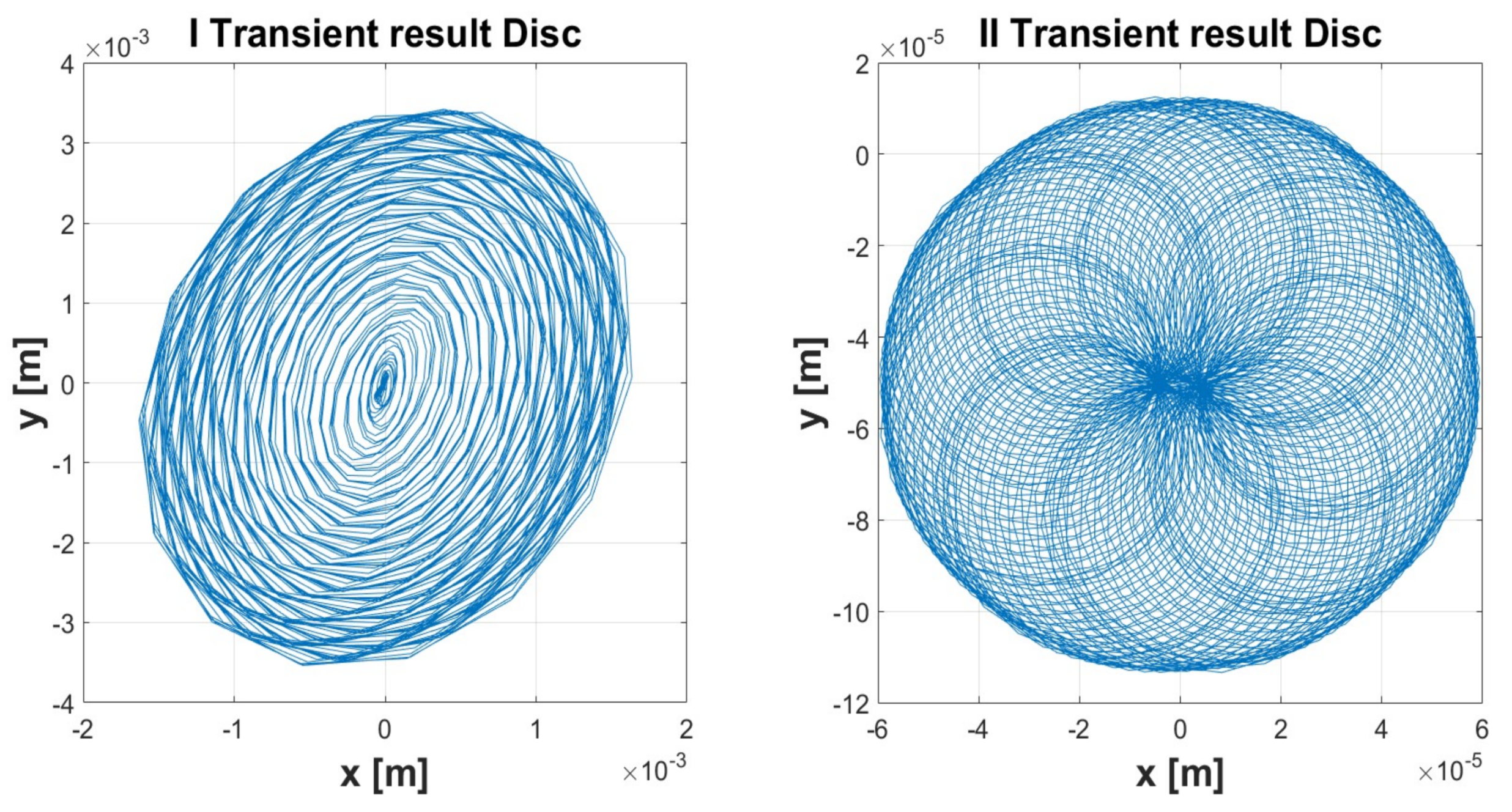
In the case of the cavitated short bearing the quality of the plots of the orbit is lower due to lower approximation in numerical integration (Figure 13). However, the orbit of the disc centre retains the extra-loop. The steady orbit of the journal centre is always circular but the radius is slightly less than the uncavitated one. The phase diagrams of the disc centre are similar, while the plots of the journal centre are completely different (Figure 14). The power spectrum (Figure 15) shows vibratory phenomena at 50 Hz and 100 Hz, therefore the system is characterized by synchronous and sub-synchronous vibrations. This power spectrum is completely different from the uncavitated one.
3.3. Simulation 3
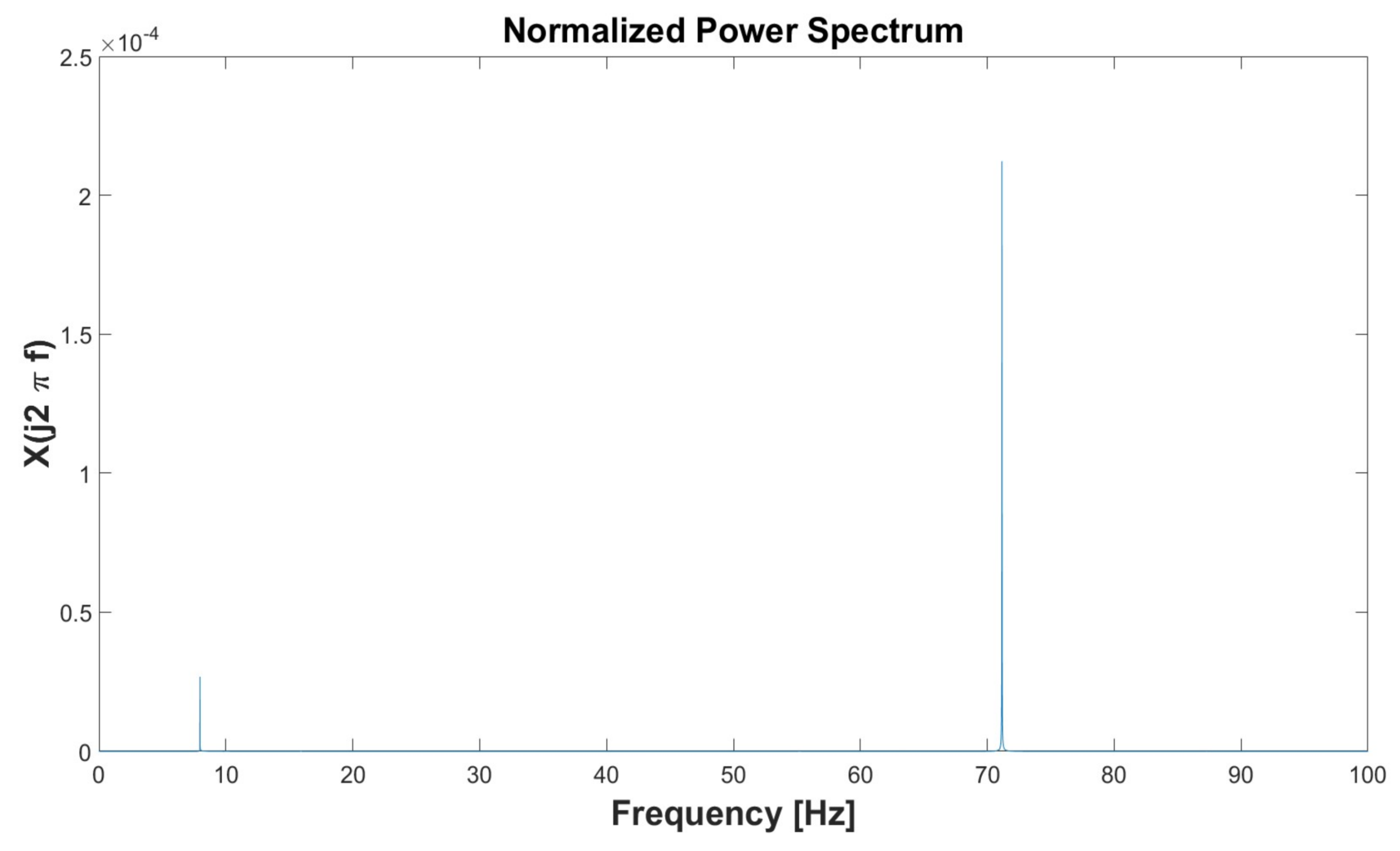
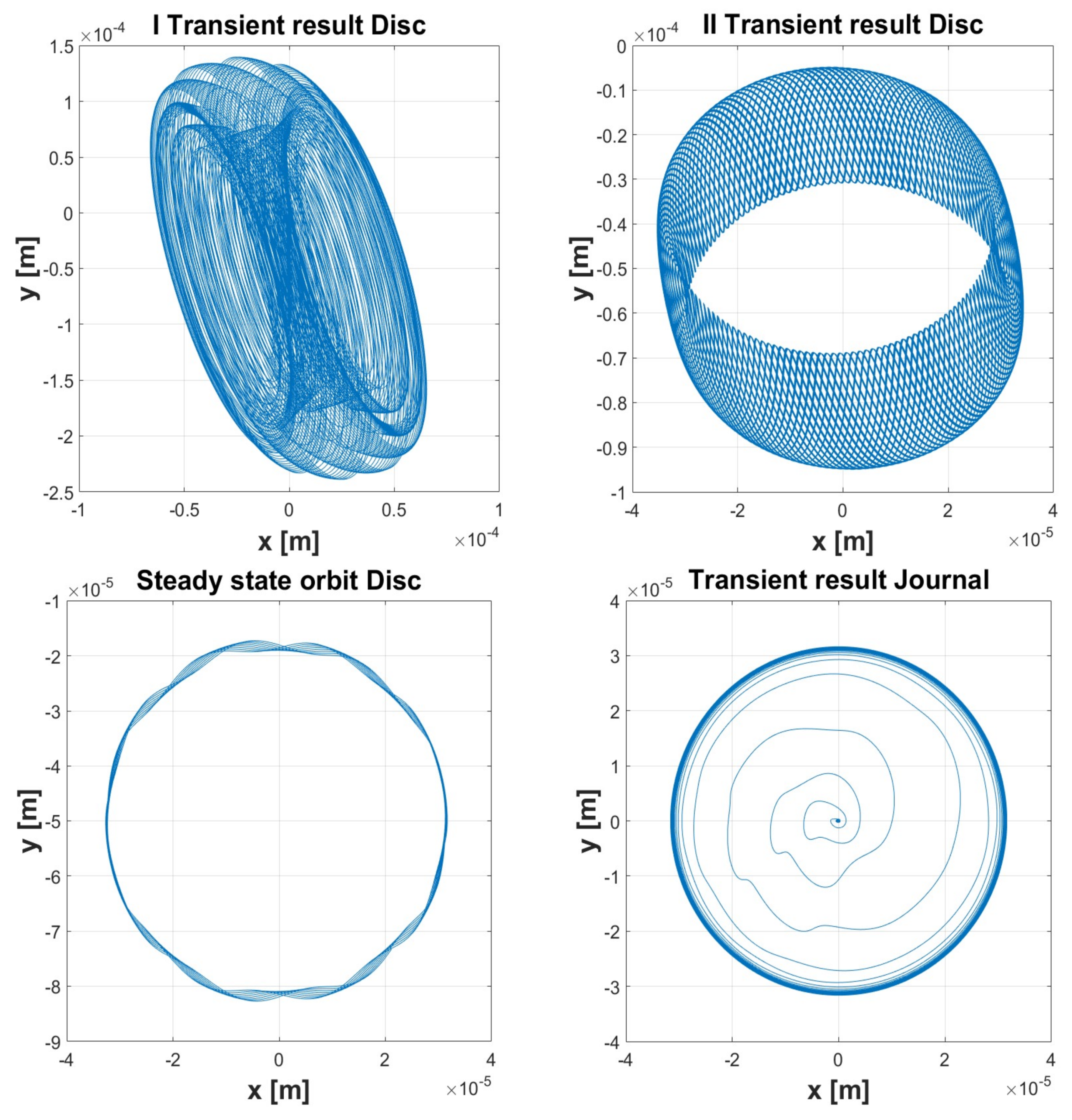
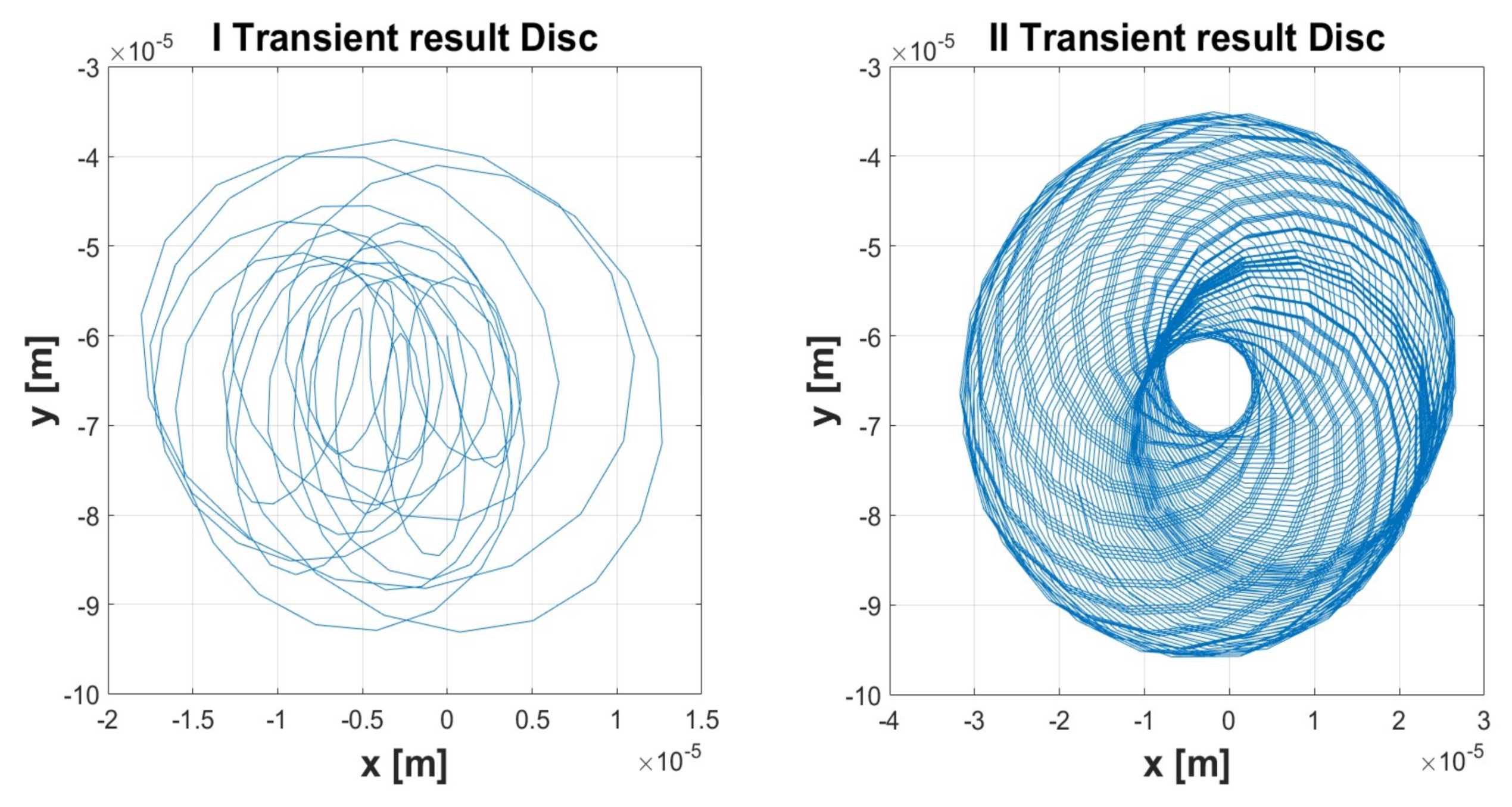
In the case of the uncavitated short bearing, the disc centre reaches the steady state in a very short time (Figure 16). The steady orbit is circular and its centre is located below the axis of the bearings (Figure 17). The dynamics of the journal centre are similar to the other cases. The discrete power spectrum (Figure 18) confirms the absence of chaos and indicates the presence of considerable vibrations at frequencies of 8 and 72 Hz.
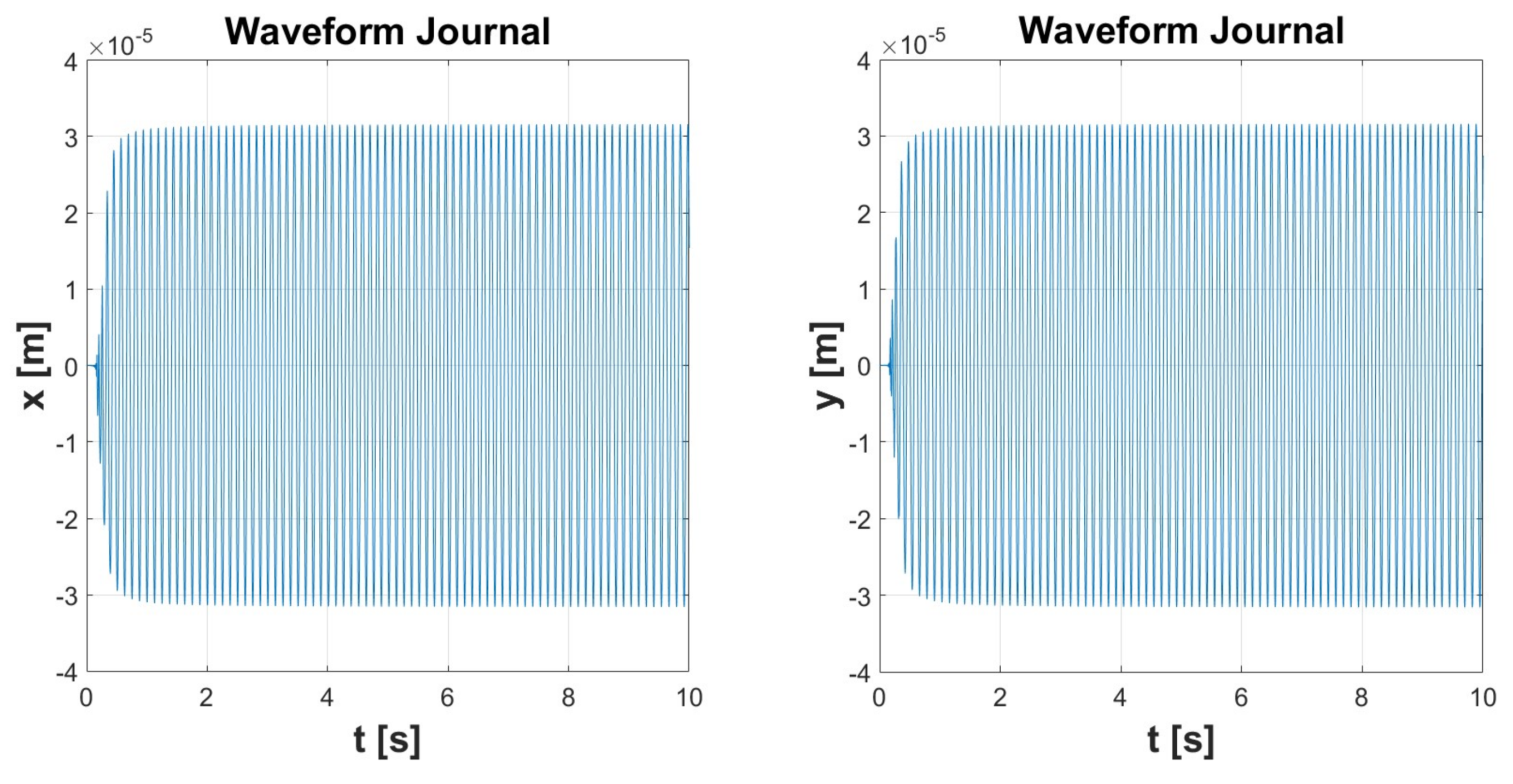
The trends for the cavitated short bearing waveforms are similar to like the uncavitated case shown in Figure 19. The disc centre does not reach a steady-state condition but the amplitude of the motion is lower (Figure 20). The journal centre always performs a circular orbit in a steady-state condition. The power spectrum (Figure 21) shows the same vibratory phenomena. However, in this case the most relevant vibration is at 8 Hz.
3.4. Simulation 4
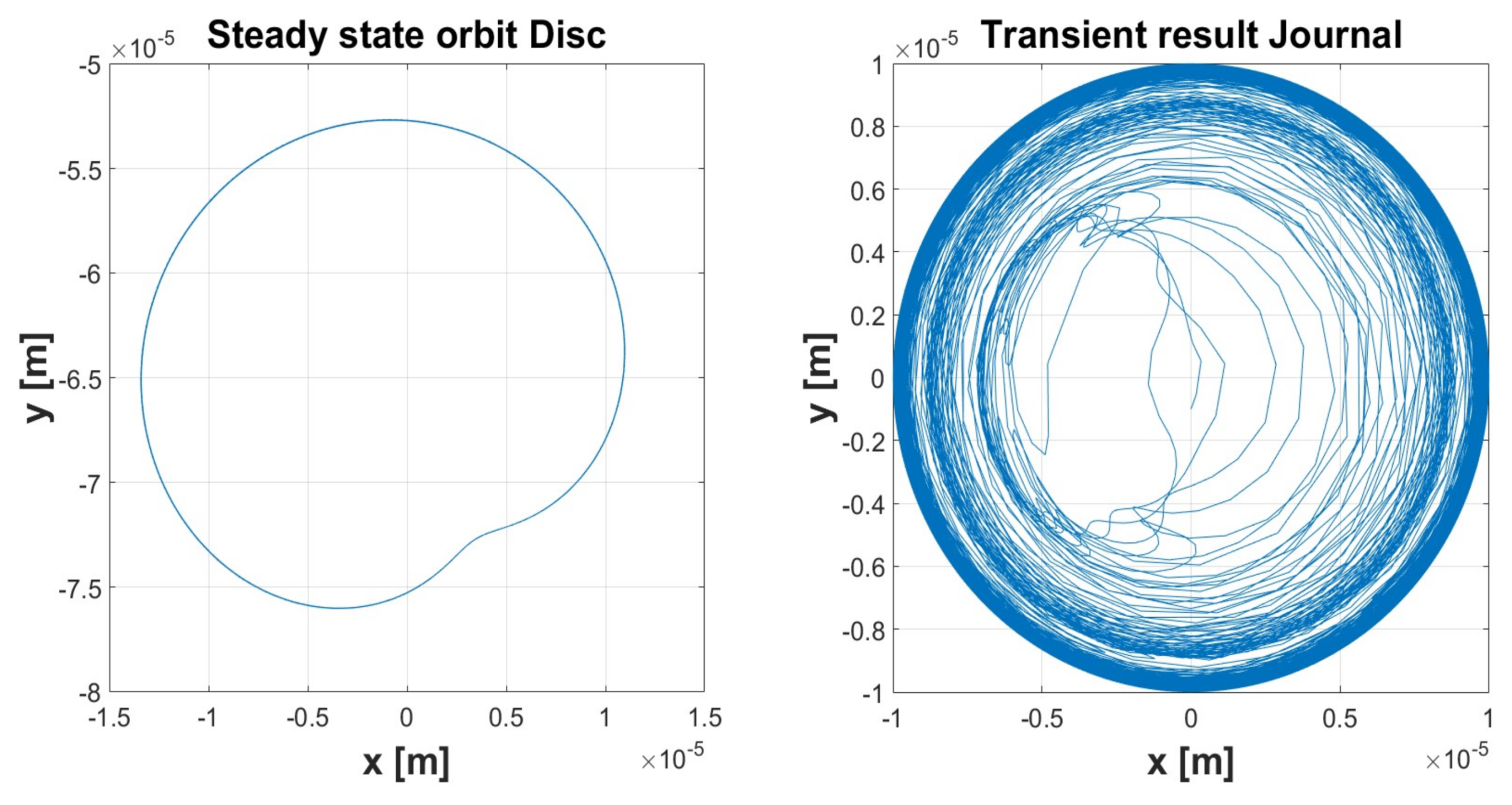
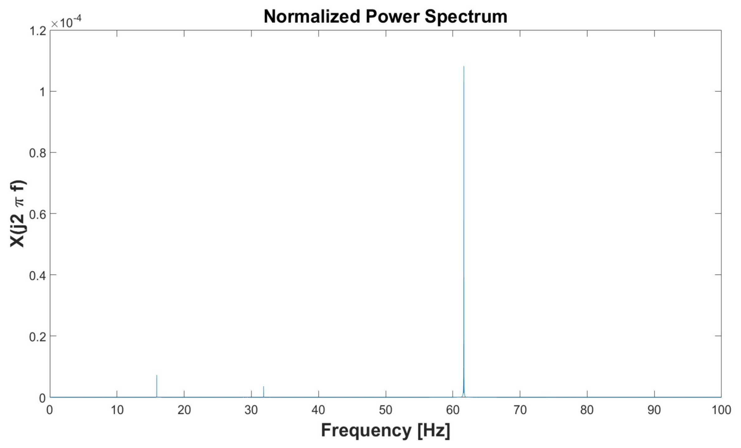
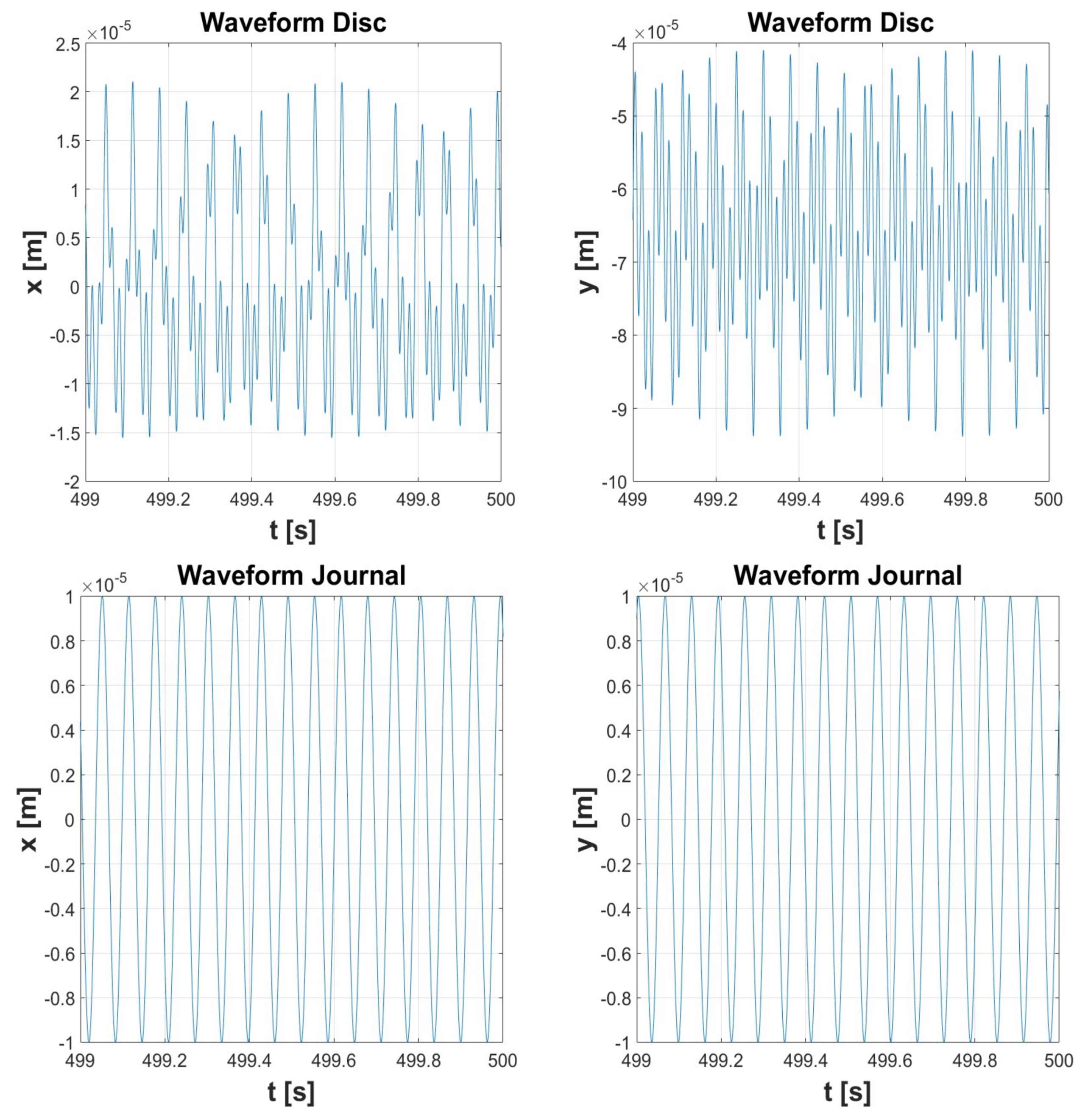
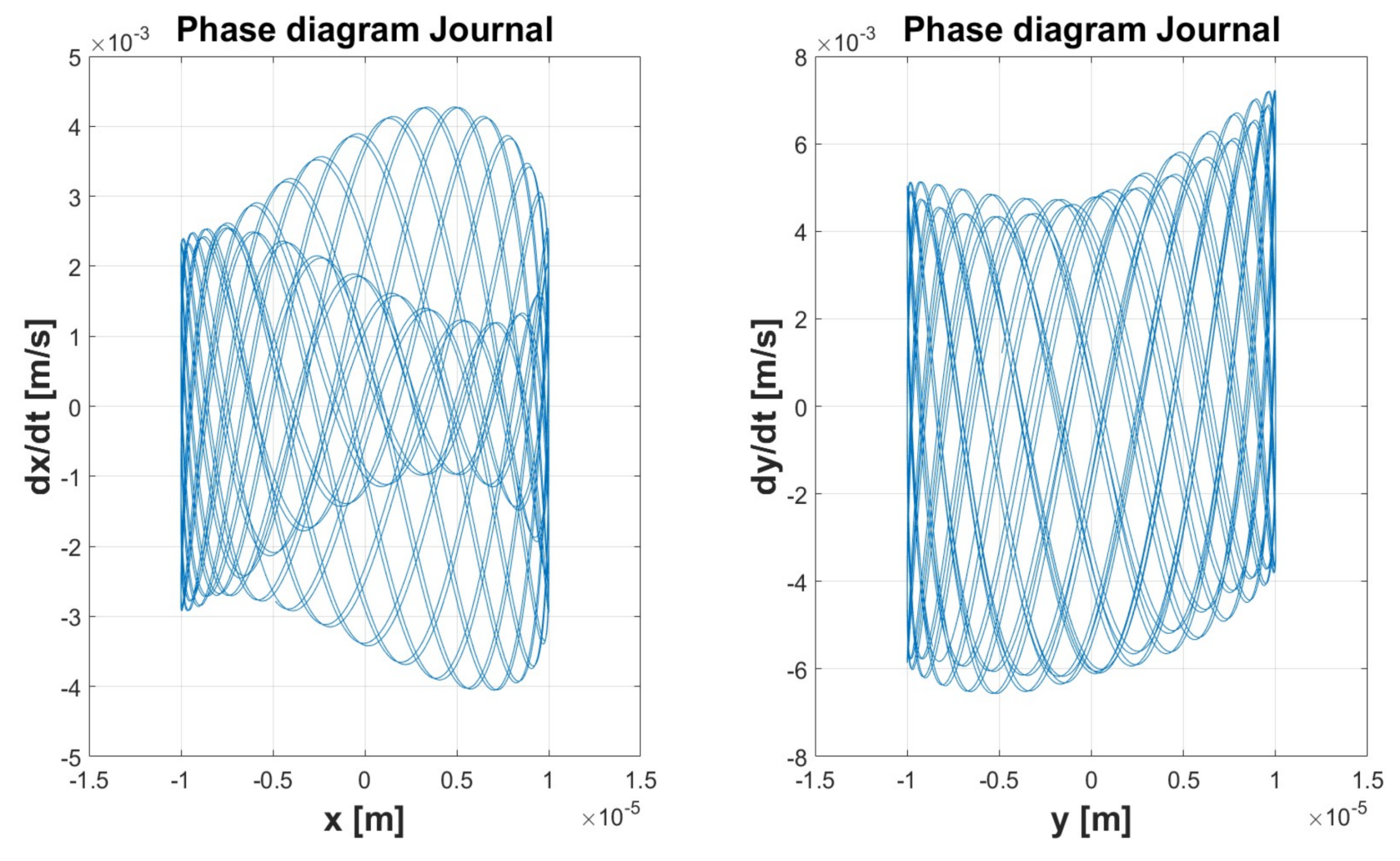
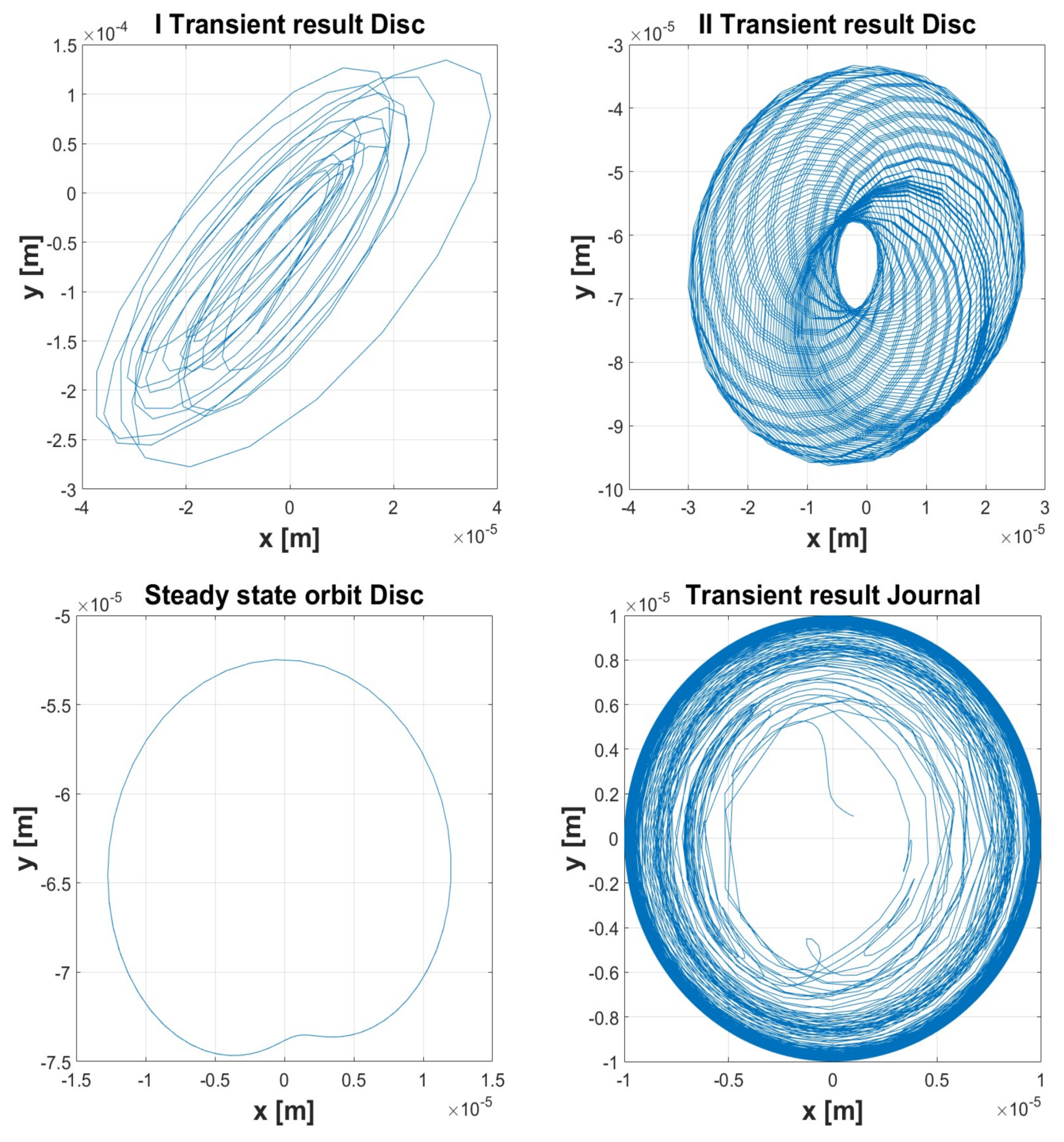
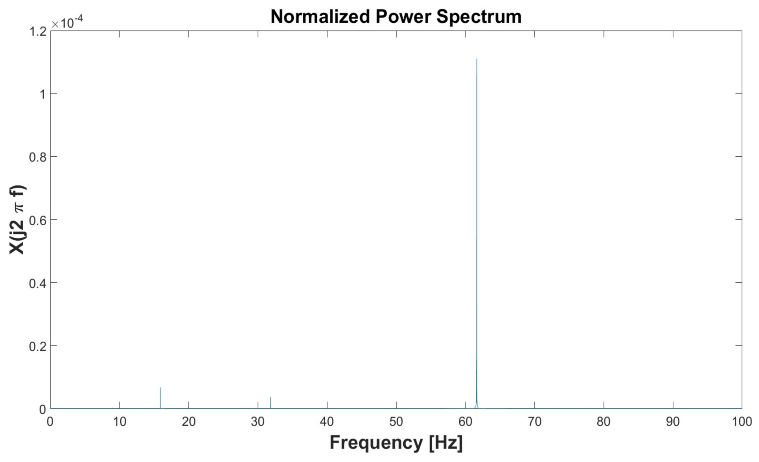
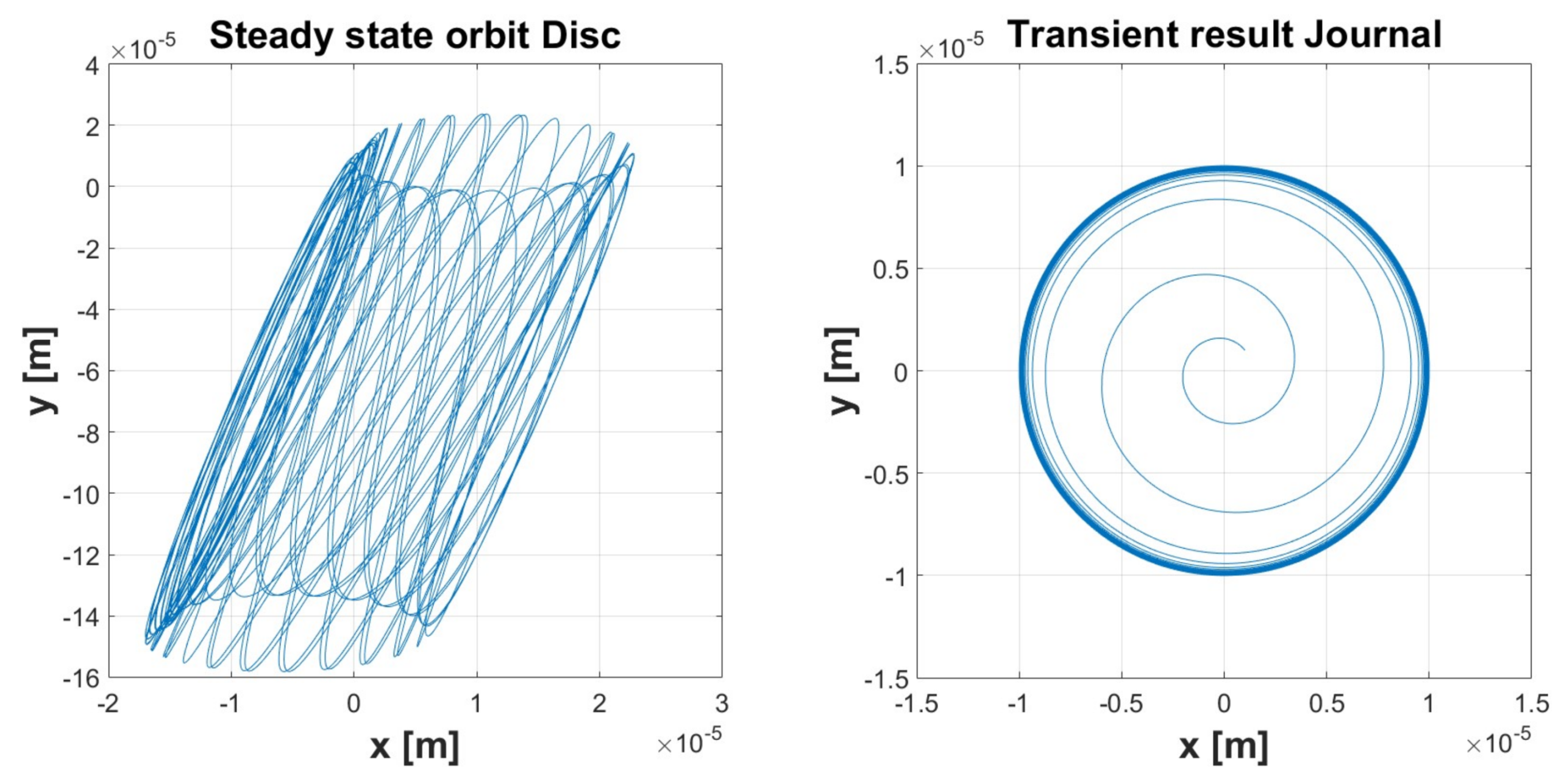
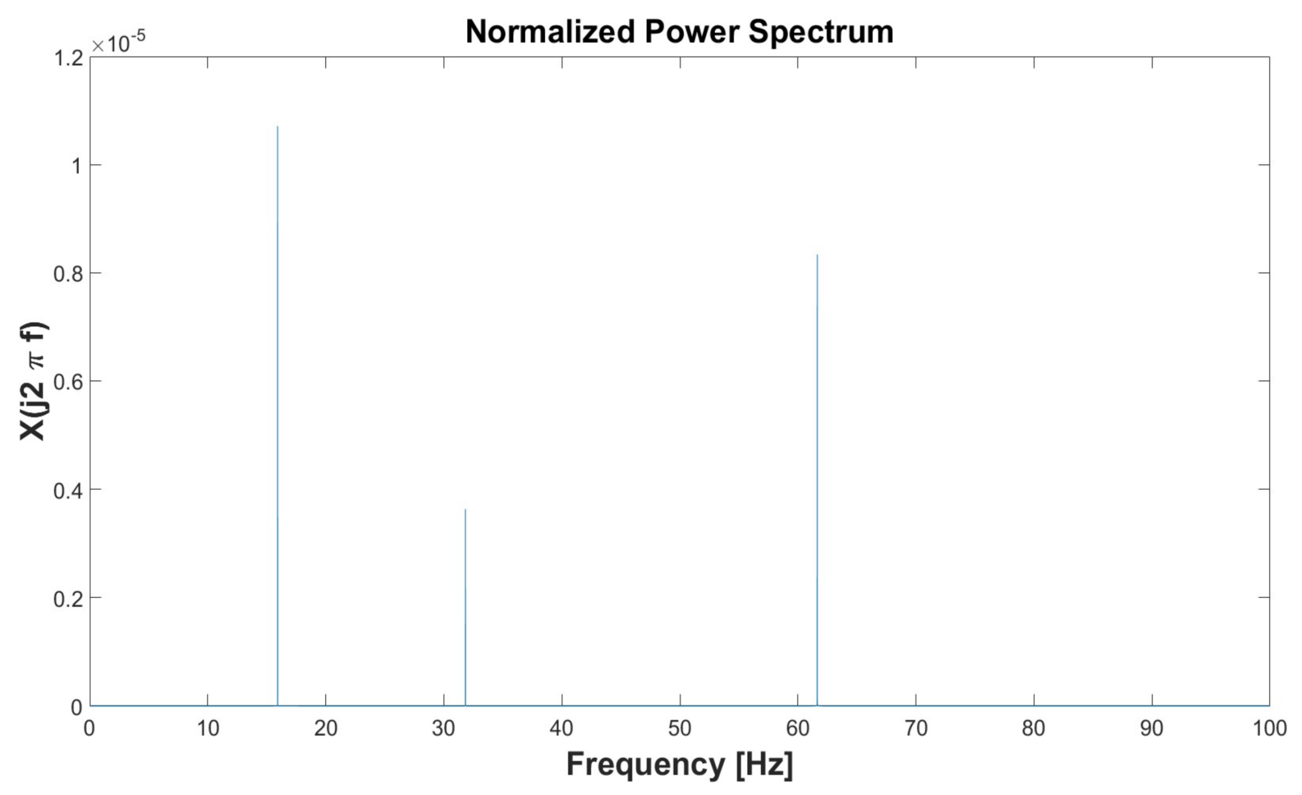
In the case of the uncavitated short bearing, it was possible to extend the simulation time. This allowed observation of a certain periodicity in the displacement diagrams (Figure 20). The Figure 22 shows the waveform of the journal. The oscillation of the centre of the disc increased every 1500 s. It reached a maximum amplitude that decreased over time, so it is possible to predict that this phenomenon is extinguished in time. Regarding the motion of the journal centre, the oscillation undergoes changes at instances in time in which there are variations of oscillation of the disc centre. This indicates that the perturbation involves the whole system. The orbit of the centre of the disc (Figure 23) is not circular. This phenomenon can be explained by analysing the power spectrum (Figure 24). The power spectrum reveals significant vibrations at frequencies near 15, 30 and 60 Hz, i.e., corresponding to ω/2, ω and 2ω. This means that the system is affected by the sub-synchronous vibrations and vibrations two per revolution. From these observations, it seems that the orbit of the disc centre has a particular form. The phase diagrams denote stability since they show well-defined closed curves (Figure 25).
In the case of the cavitated short bearing, the motion of the disc centre is not characterized by periodic phenomena as in the uncavitated short bearing. As can be observed from the detail of the waveform, the oscillation is strongly non-linear (Figure 26). The orbits of the disc centre are completely different (Figure 27). The transient of the journal centre is different, but the steady orbit is almost the same. Even the phase diagrams are completely different (Figure 28). The power spectrum shows some common vibratory phenomena (Figure 29).
3.5. Simulation 5
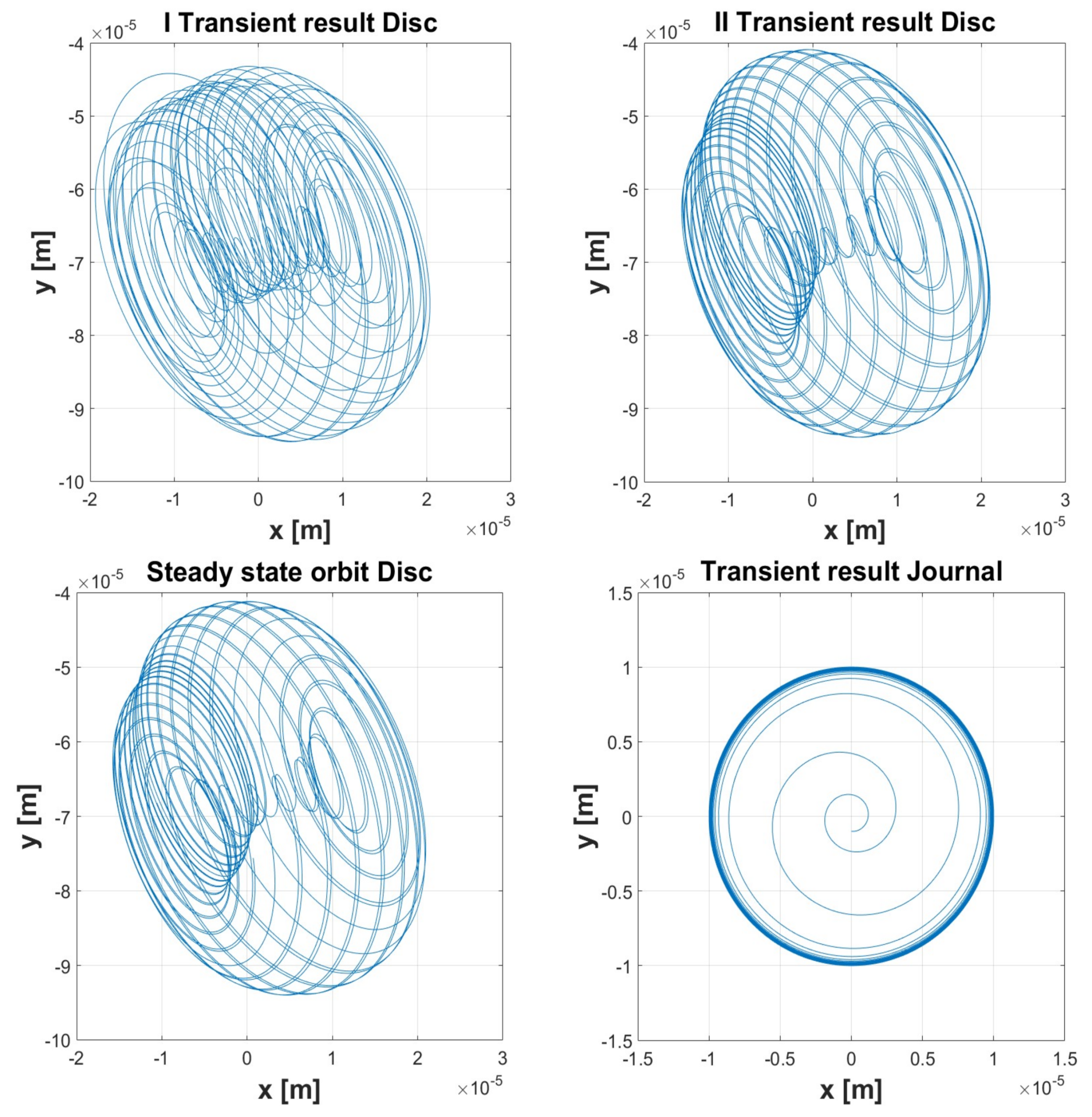
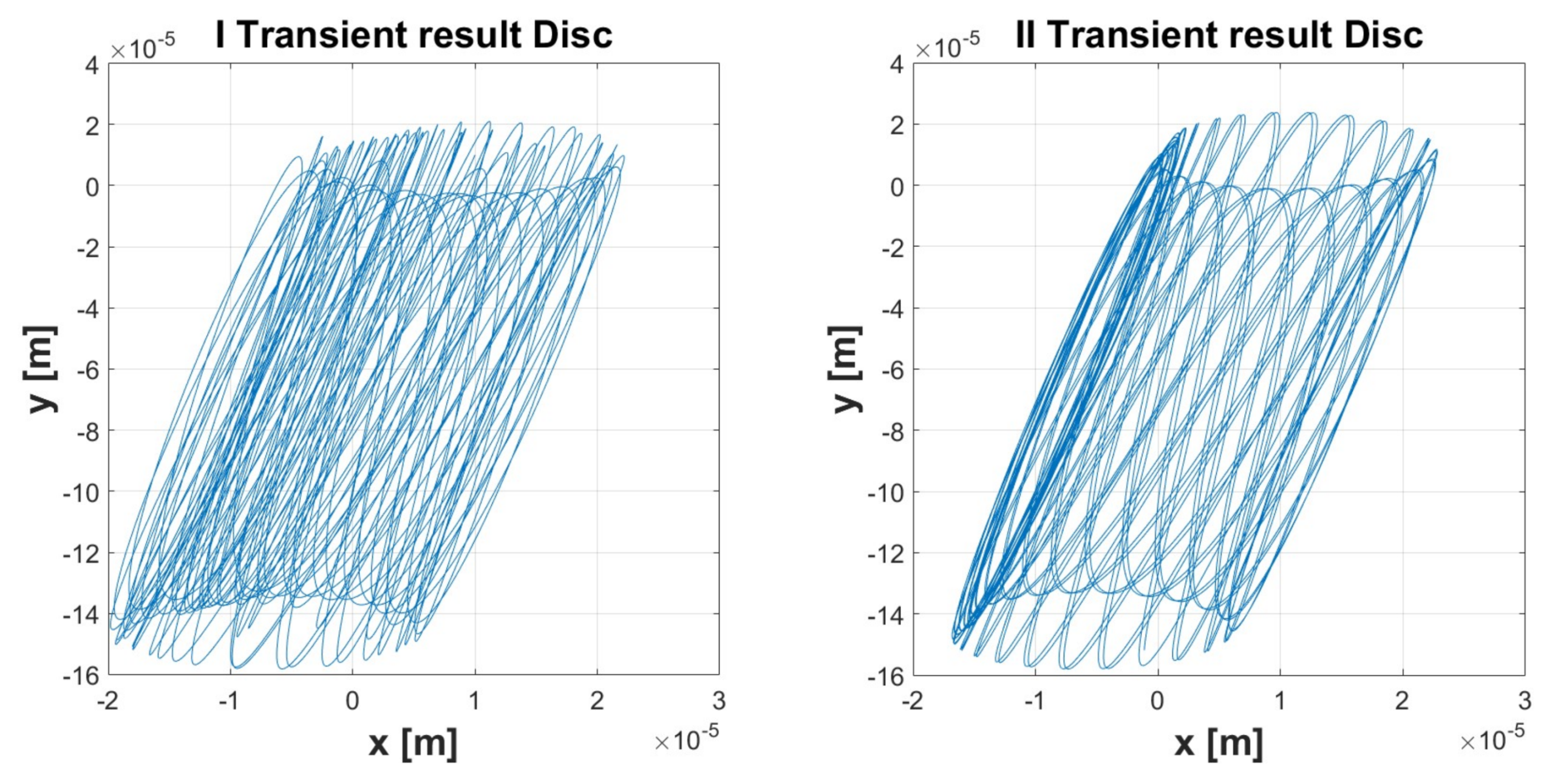
This simulation was conducted by assigning the same values from Simulation 4 to the parameters, except for the initial conditions. This was done in order to highlight the characteristics of dynamical systems, where two identical systems with similar initial conditions show different resulting motions. This feature can be observed in the plot of the orbits and in the phase diagrams (Figure 30, Figure 31, Figure 32, Figure 33, Figure 34 and Figure 35).
4. Conclusions
In this paper, the dynamic behaviour of a thin disk splined in the middle of a flexible rotor supported by hydrodynamic bearings was analysed. To make mathematical expressions easier, the fluid film forces, exerted by the bearings on the journal in hydrodynamic lubrication conditions, have been previously defined under the hypothesis of short bearings.
The equations of motion have been written considering the dynamic balance of the rotor system consisting of a shaft and a disc. As the equations of motion are characterized by a strong non-linearity, it is necessary to use a computer code for the numerical integration. For this purpose, the Matlab-Simulink environment allowed calculation of the numerical results. The study of the rotor-bearing system, both in the presence and absence of cavitation enabled us to compare these two journal bearings models to understand how the cavitation phenomenon can influence the system dynamics.
The results show that cavitation significantly influences the dynamic behaviour of the rotor system. The waveform changes considerably, especially for the centre of the disc, and leads to completely different orbits in the two cases studied. However, the order of magnitude of the orbits remains almost the same, at least in the simulations performed, so cavitation should not cause problems with bulkheads.
The most significant effect is found by analysing the power spectra as the effect of cavitation changes the frequencies and intensity of the vibrating phenomena.
The Cavitated (π-Film) Short Bearing model responds quite well and can be used as a predictive tool for the dynamic behaviour of a rotor system such as the one treated, especially to avoid critical events such as flexural resonance.
Author Contributions
Alessandro Ruggiero, Roberto D’Amato and Drazan Kozak wrote this article. Alessandro Ruggiero and Emanuele Magliano developed the simulation tools and conducted the simulations. Roberto D’Amato and Drazan Kozak supervised the simulation results. The academic background was provided by Alessandro Ruggiero. Alessandro Ruggiero, Roberto D’Amato, Emanuele Magliano and Drazan Kozak have analysed the results and wrote the conclusions.
Conflicts of Interest
The authors declare no conflict of interest.
Nomenclature
| 2m | disc mass |
| Ks | shaft bending stiffness |
| 2W | static load |
| O | bearing centre |
| J | journal centre |
| C | disc geometric centre |
| M | disc centre of gravity |
| u | disc static imbalance |
| R | journal radius |
| r | disc radius |
| L | bearing length |
| c | radial bearing clearance |
| e | eccentricity |
| eccentricity ratio | |
| δ | shaft deflection |
| ω | disc angular velocity |
| μ | lubricant viscosity |
| ω | angular velocity of the journal (constant) |
| attitude angle | |
| k | flexural stiffness of the shaft |
| angular velocity of the line of centres (journal whirling) | |
| (xc,yc) | disc centre coordinates |
| (xj,yj) | journal centre coordinates |
References
- Friswell, M.I.; Penny, J.E.T.; Garvey, S.D.; Lees, A.W. Dynamics of Rotating Machines; Cambridge University Press: Cambridge, UK, 2010; ISBN 9780511780509. [Google Scholar]
- Lund, J.W. Review of the Concept of Dynamic Coefficients for Fluid Film Journal Bearings. J. Tribol. 1987, 109, 37. [Google Scholar] [CrossRef]
- Muszynska, A. Stability of whirl and whip in rotor/bearing systems. J. Sound Vib. 1988, 127, 49–64. [Google Scholar] [CrossRef]
- D’Agostino, V.; Guida, D.; Ruggiero, A.; Senatore, A. An analytical study of the fluid film force in finite-length journal bearings. Part I. Lubr. Sci. 2001, 13, 329–340. [Google Scholar] [CrossRef]
- Poritsky, H. Contribution to the theory of oil whip. Trans. ASME 1953, 75, 1153–1161. [Google Scholar]
- Huang, T.-W.; Weng, C.-T. Dynamic characteristics of finite-width journal bearings with micropolar fluids. Wear 1990, 141, 23–33. [Google Scholar] [CrossRef]
- Bansal, P.; Chattopadhayay, A.K.; Agrawal, V.P. Linear Stability Analysis of Hydrodynamic Journal Bearings with a Flexible Liner and Micropolar Lubrication. Tribol. Trans. 2015, 58, 316–326. [Google Scholar] [CrossRef]
- Naduvinamani, N.B.; Hiremath, P.S.; Gurubasavaraj, G. Static and dynamic behaviour of squeeze-film lubrication of narrow porous journal bearings with coupled stress fluid. Proc. Inst. Mech. Eng. Part J J. Eng. Tribol. 2001, 215, 45–62. [Google Scholar] [CrossRef]
- Naduvinamani, N.B.; Marali, G.B. Dynamic Reynolds equation for micropolar fluids and the analysis of plane inclined slider bearings with squeezing effect. Proc. Inst. Mech. Eng. Part J J. Eng. Tribol. 2007, 221, 823–829. [Google Scholar] [CrossRef]
- Das, S.; Guha, S.K.; Chattopadhyay, A.K. Linear stability analysis of hydrodynamic journal bearings under micropolar lubrication. Tribol. Int. 2005, 38, 500–507. [Google Scholar] [CrossRef]
- Harika, E.; Bouyer, J.; Fillon, M.; Hélène, M. Measurements of lubrication characteristics of a tilting pad thrust bearing disturbed by a water-contaminated lubricant. Proc. Inst. Mech. Eng. Part J J. Eng. Tribol. 2013, 227, 16–25. [Google Scholar] [CrossRef]
- Vania, A.; Pennacchi, P.; Chatterton, S. Dynamic Effects Caused by the Non-Linear Behavior of Oil-Film Journal Bearings in Rotating Machines. In Proceedings of the ASME Turbo Expo 2012: Turbine Technical Conference and Exposition (Volume 7: Structures and Dynamics, Parts A and B), Copenhagen, Denmark, 11–15 June 2012; ASME: New York, NY, USA, 2012; p. 657. [Google Scholar]
- Harika, E.; Bouyer, J.; Fillon, M.; Hélène, M. Effects of Water Contamination of Lubricants on Hydrodynamic Lubrication: Rheological and Thermal Modeling. J. Tribol. 2013, 135, 41707. [Google Scholar] [CrossRef]
- Sukumaran Nair, V.P.; Prabhakaran Nair, K. Finite element analysis of elastohydrodynamic circular journal bearing with micropolar lubricants. Finite Elem. Anal. Des. 2004, 41, 75–89. [Google Scholar] [CrossRef]
- Lin, T.-R. Hydrodynamic lubrication of journal bearings including micropolar lubricants and three-dimensional irregularities. Wear 1996, 192, 21–28. [Google Scholar] [CrossRef]
- Prabhakaran Nair, K.; Sukumaran Nair, V.P.; Jayadas, N.H. Static and dynamic analysis of elastohydrodynamic elliptical journal bearing with micropolar lubricant. Tribol. Int. 2007, 40, 297–305. [Google Scholar] [CrossRef]
- Pennacchi, P.; Vania, A.; Chatterton, S. Nonlinear effects caused by coupling misalignment in rotors equipped with journal bearings. Mech. Syst. Signal Process. 2012, 30, 306–322. [Google Scholar] [CrossRef] [Green Version]
- Lund, J.W.; Sternlicht, B. Rotor-Bearing Dynamics with Emphasis on Attenuation. J. Basic Eng. 1962, 84, 491. [Google Scholar] [CrossRef]
- Pinkus, O. The Reynolds Centennial: A Brief History of the Theory of Hydrodynamic Lubrication. J. Tribol. 1987, 109, 2. [Google Scholar] [CrossRef]
- Szeri, A.Z. Some Extensions of the Lubrication Theory of Osborne. J. Tribol. 1987, 109, 21–36. [Google Scholar] [CrossRef]
- Nitzschke, S.; Woschke, E.; Daniel, C.; Strackeljan, J. Einfluss der masseerhaltenden Kavitation auf gleitgelagerte Rotoren unter instationärer Belastung. In Proceedings of the SIRM 2013-10, Internationale Tagung Schwingungen in Rotierenden Maschinen, Berlin, Germany, 25–27 February 2013; p. ID-210. [Google Scholar]
- Ruggiero, A.; Gómez, E.; D’Amato, R. Approximate closed-form solution of the synovial fluid film force in the human ankle joint with non-Newtonian lubricant. Tribol. Int. 2013, 57, 156–161. [Google Scholar] [CrossRef]
- Ruggiero, A.; Hloch, S.; Kozak, D.; Valasek, P. Analytical fluid film force calculation in the case of short bearing with a fully developed turbulent flow. Proc. Inst. Mech. Eng. Part J J. Eng. Tribol. 2016, 230, 395–401. [Google Scholar] [CrossRef]
- Van der Pol, B.; Van der Mark, J. The heartbeat considered as a relaxation oscillation, and an electrical model of the heart. Lond. Edinb. Dublin Philos. Mag. J. Sci. 1928, 6, 763–775. [Google Scholar] [CrossRef]
- Thompson, J.M.T.; Stewart, H.B. Nonlinear Dynamics and Chaos; Wiley: Hoboken, NJ, USA, 2002; ISBN 0471876453. [Google Scholar]
- Vance, J.M. Rotordynamics of Turbomachinery; Wiley: Hoboken, NJ, USA, 1988; ISBN 0471802581. [Google Scholar]
Figure 1.
Scheme of rotor bearing system.
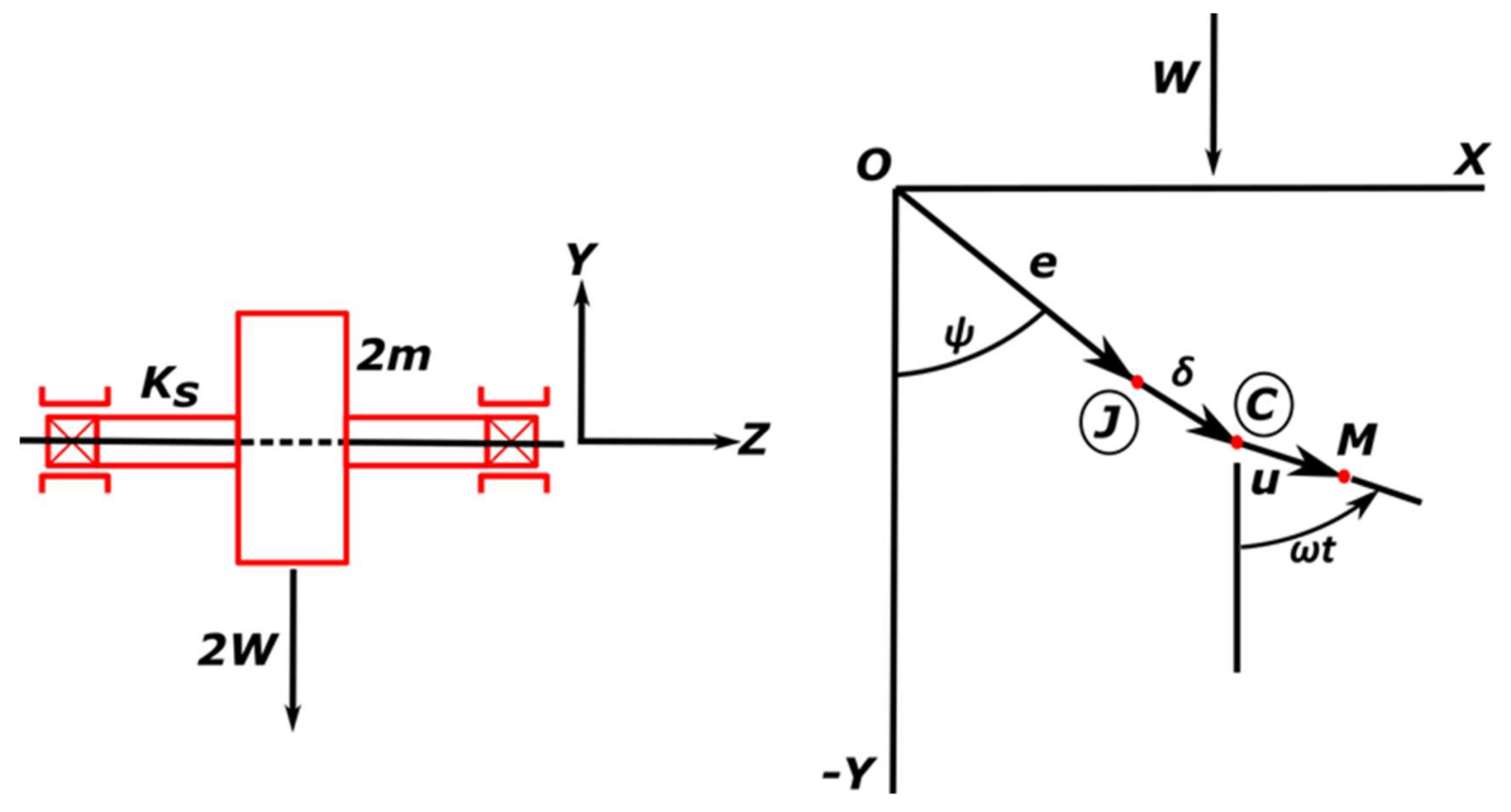
Figure 2.
Journal bearing geometry.
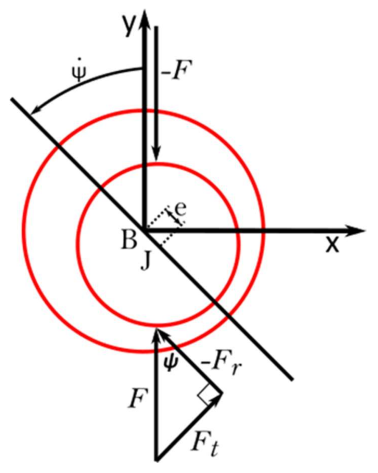
Figure 3.
Simulink algorithm scheme for the uncavitated short bearing.
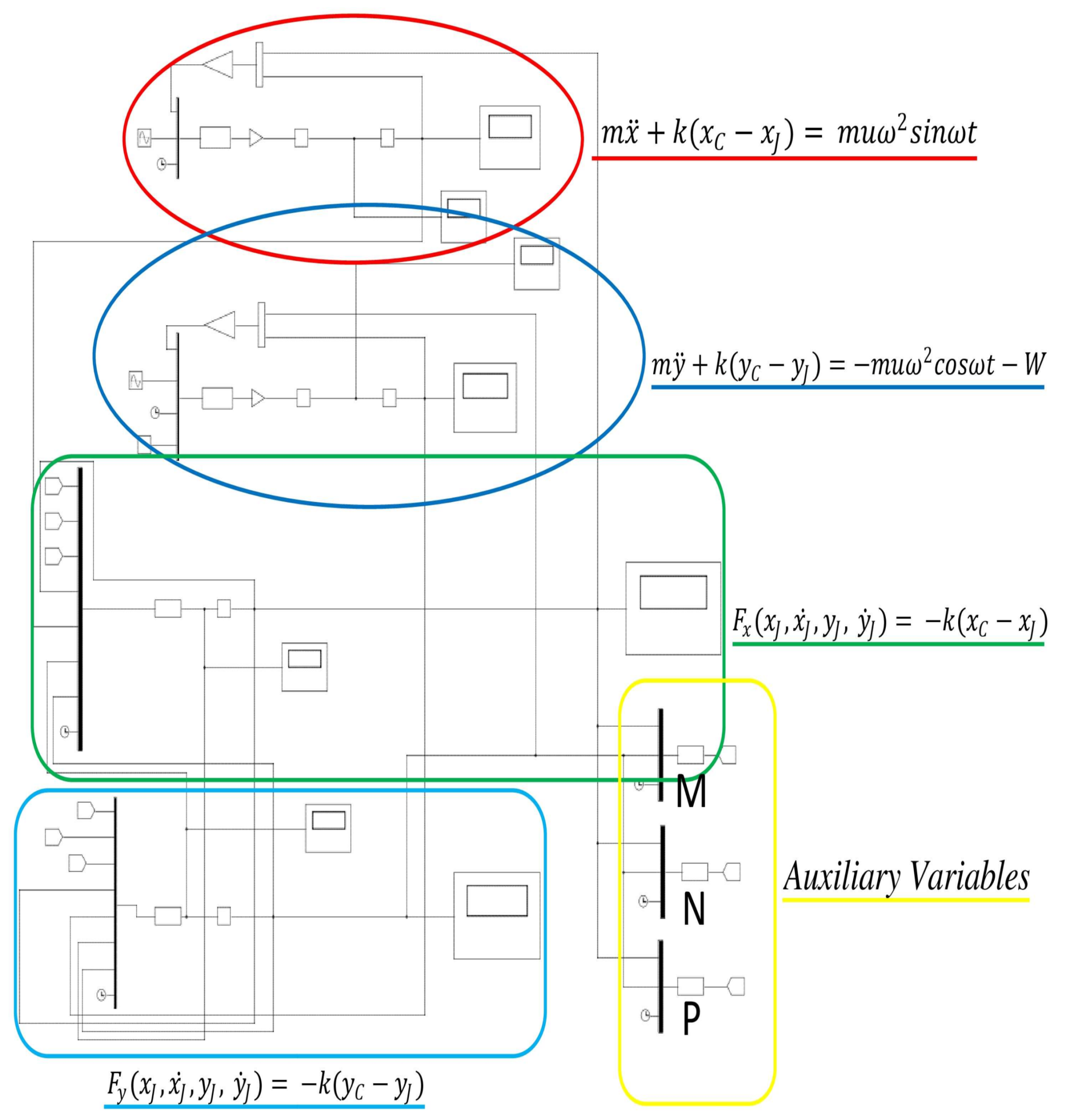
Figure 4.
Simulink algorithm scheme—detail of Equation (10).

Figure 5.
Simulink algorithm scheme—detail of Equation (13). The variables (a,b) represent the coordinates of the centre of the journal (xj,yj).
Figure 5.
Simulink algorithm scheme—detail of Equation (13). The variables (a,b) represent the coordinates of the centre of the journal (xj,yj).

Figure 6.
Simulation 1: Uncavitated—Orbits.
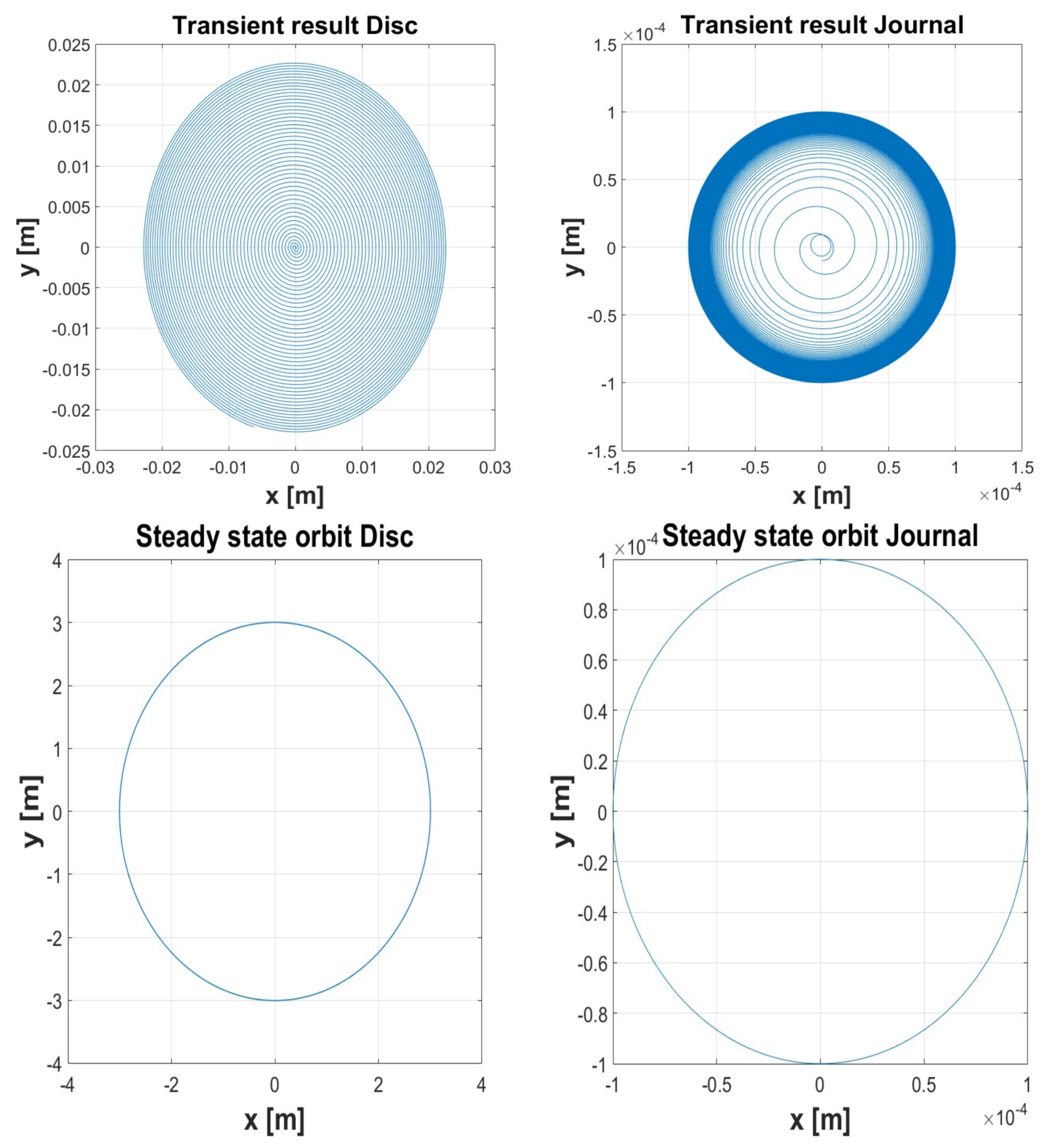
Figure 7.
Simulation 1: Uncavitated—Normalized Power Spectrum.
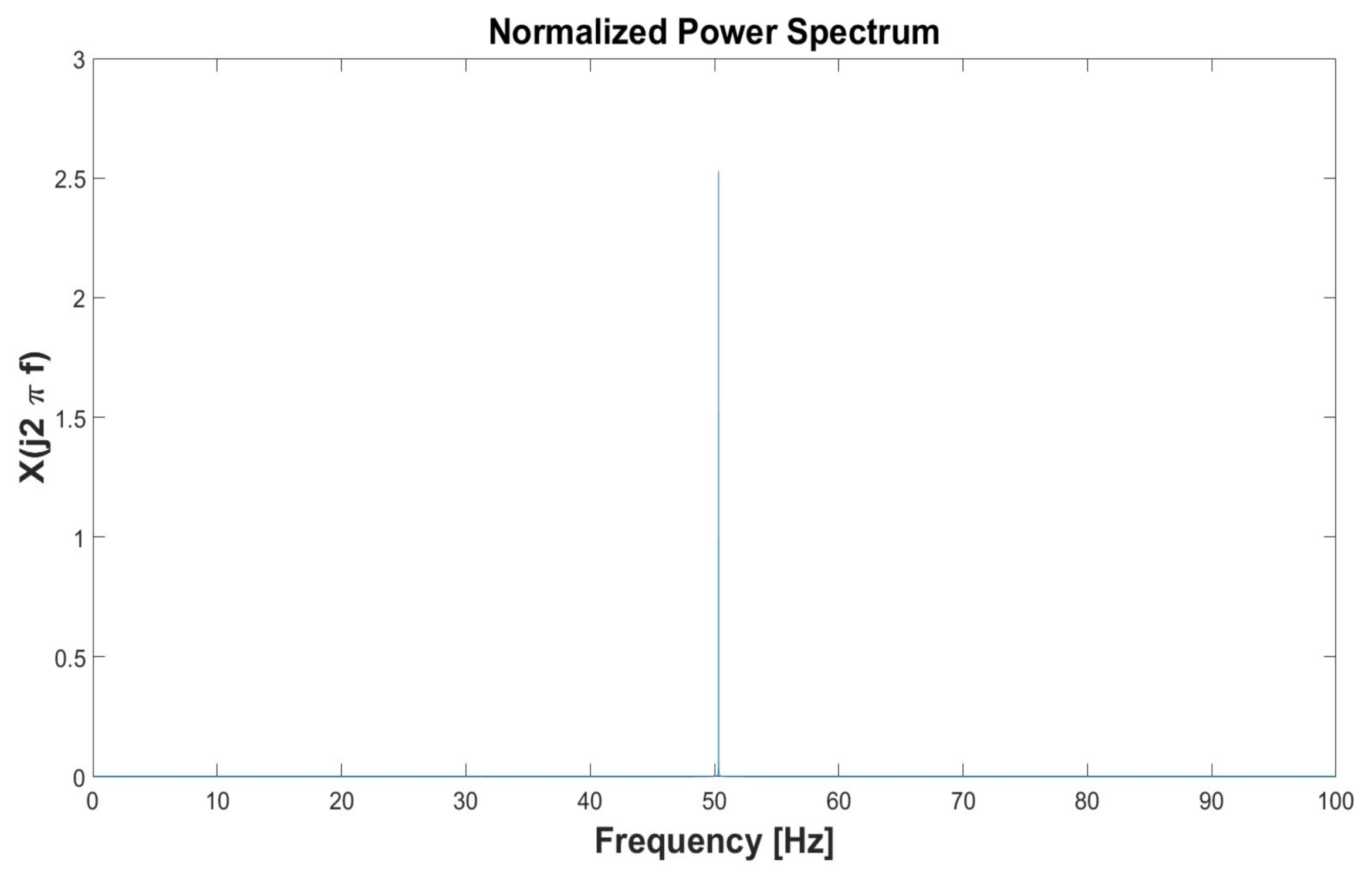
Figure 8.
Simulation 1: Cavitated—Orbits.

Figure 9.
Simulation 1: Cavitated—Normalized Power Spectrum.

Figure 10.
Simulation 2: Uncavitated—Orbits.
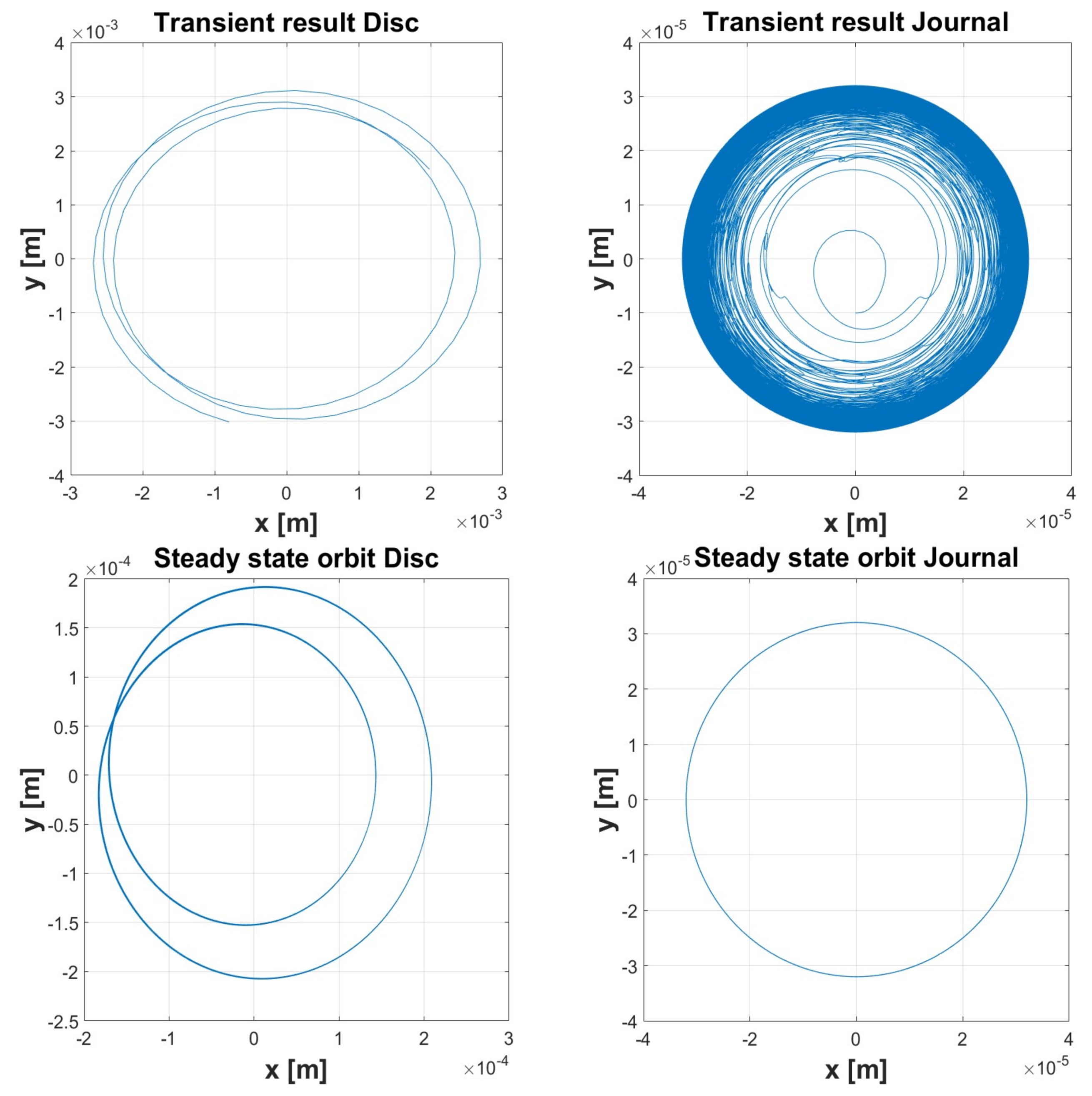
Figure 11.
Simulation 2: Uncavitated—Phase Diagrams.
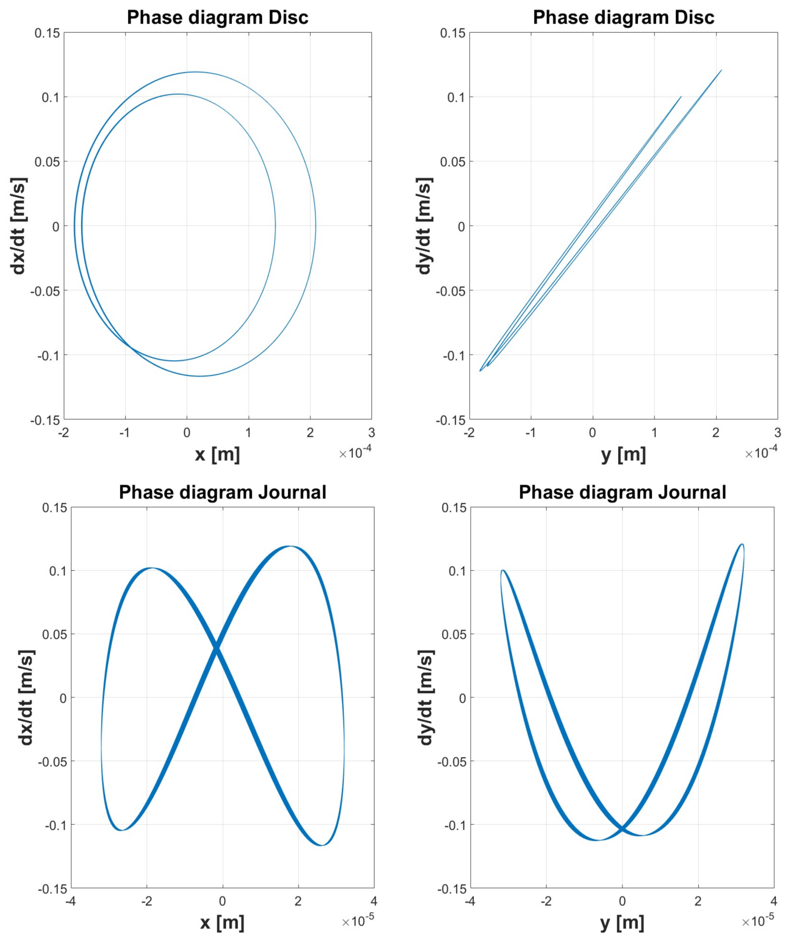
Figure 12.
Simulation 2: Uncavitated—Normalized Power Spectrum.
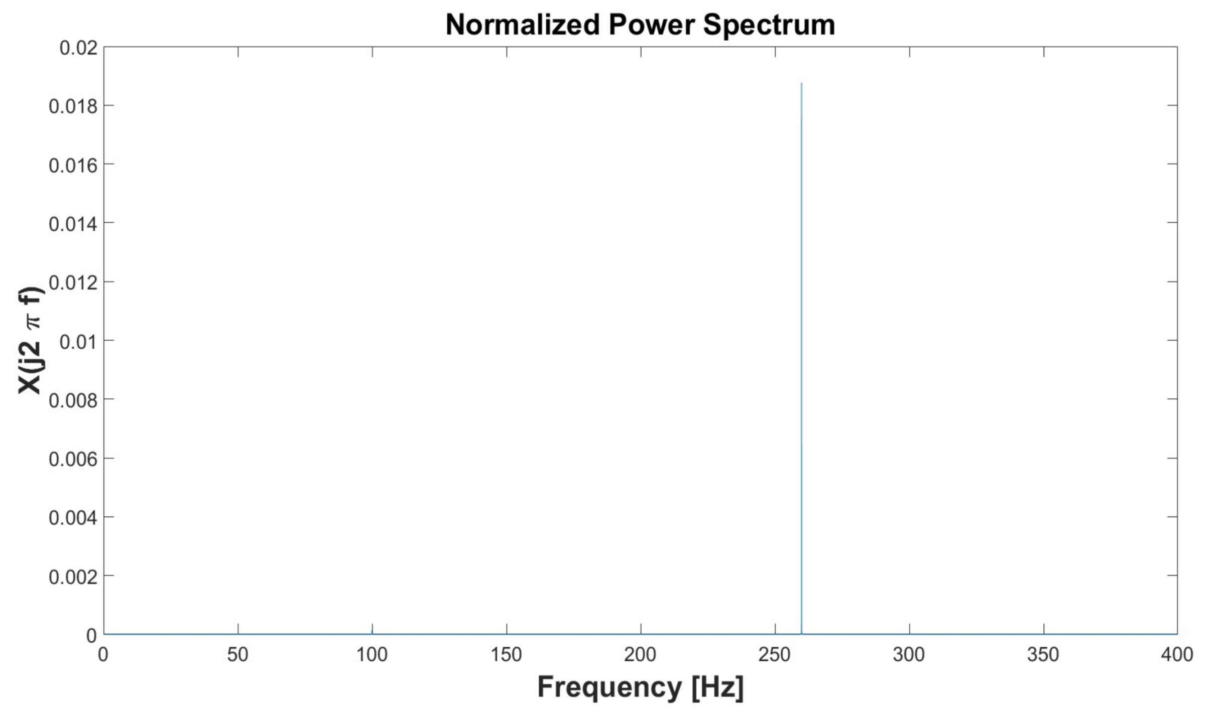
Figure 13.
Simulation 2: Cavitated—Orbits.

Figure 14.
Simulation 2: Cavitated—Phase Diagrams.
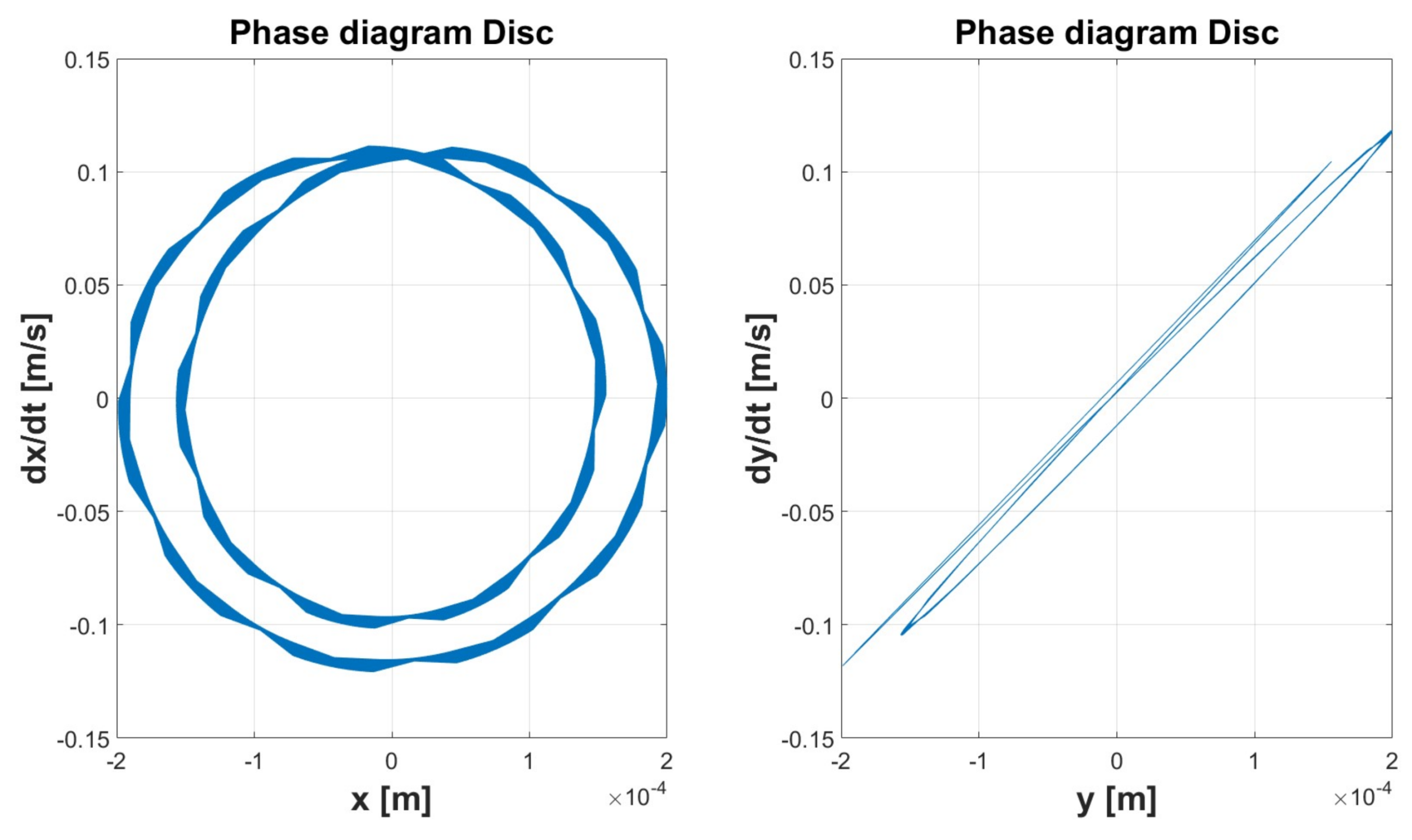

Figure 15.
Simulation 2: Cavitated—Normalized Power Spectrum.

Figure 16.
Simulation 3: Uncavitated—Waveforms.

Figure 17.
Simulation 3: Uncavitated—Orbits.


Figure 18.
Simulation 3: Uncavitated—Normalized Power Spectrum.

Figure 19.
Simulation 3: Cavitated—Waveforms.
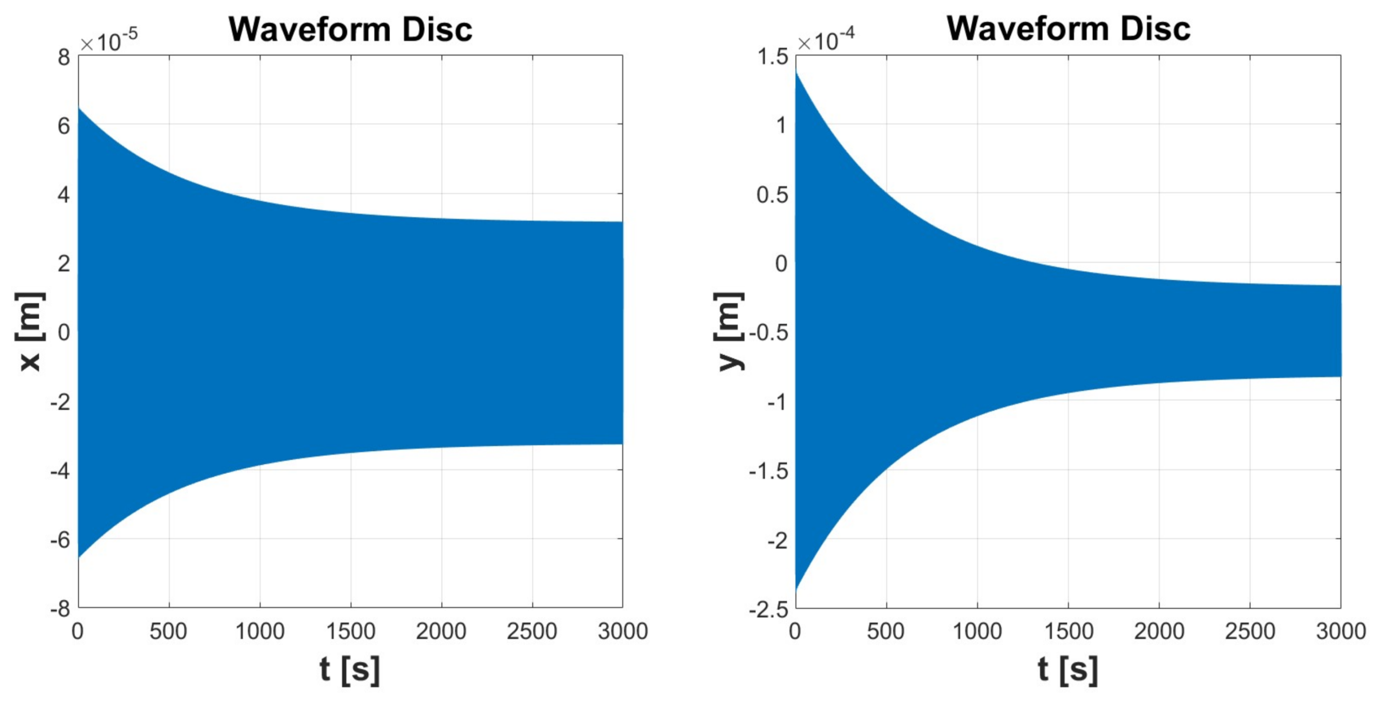

Figure 20.
Simulation 3: Cavitated—Orbits.

Figure 21.
Simulation 3: Cavitated—Normalized Power Spectrum.
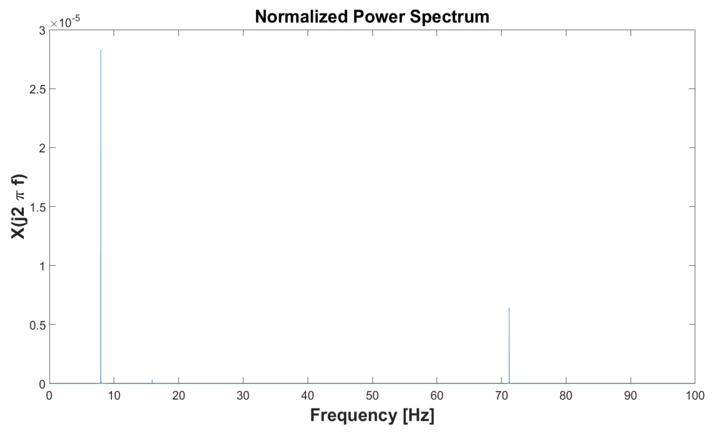
Figure 22.
Simulation 4: Uncavitated—Waveforms.
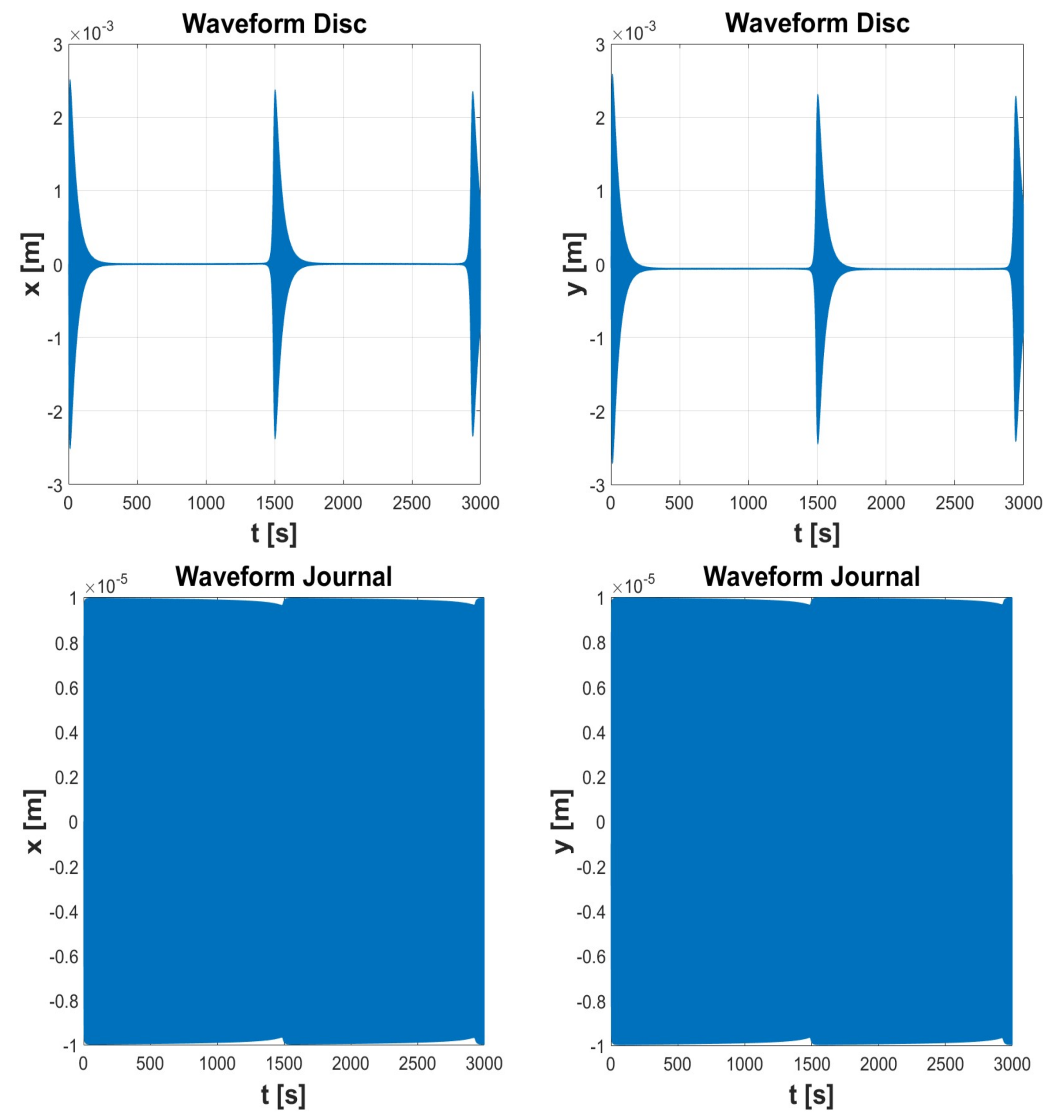
Figure 23.
Simulation 4: Uncavitated—Orbits.


Figure 24.
Simulation 4: Uncavitated—Normalized Power Spectrum.

Figure 25.
Simulation 4: Uncavitated—Phase Diagrams.
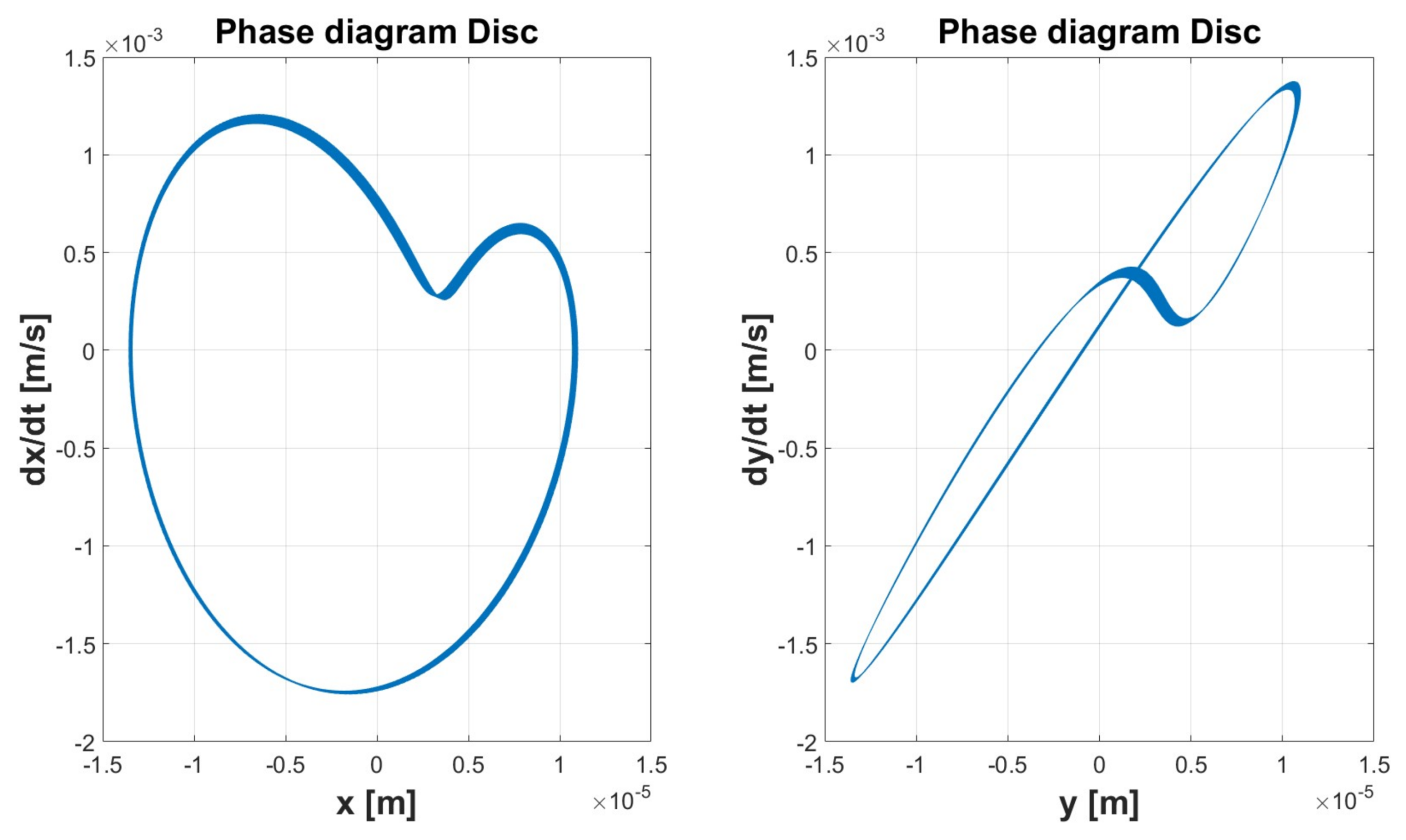
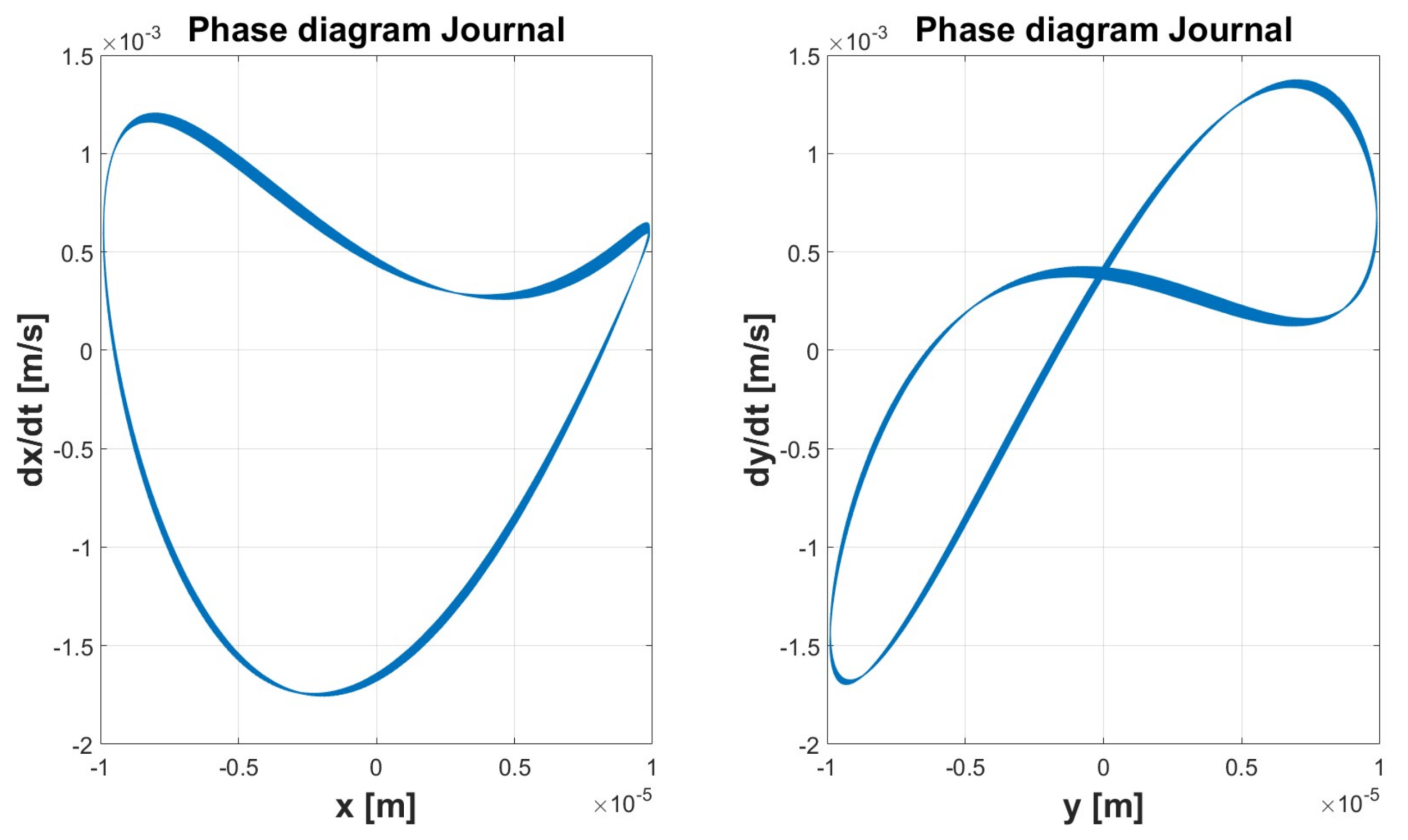
Figure 26.
Simulation 4: Cavitated—Waveforms Detail.

Figure 27.
Simulation 4: Cavitated—Orbits.

Figure 28.
Simulation 4: Cavitated—Phase Diagrams.
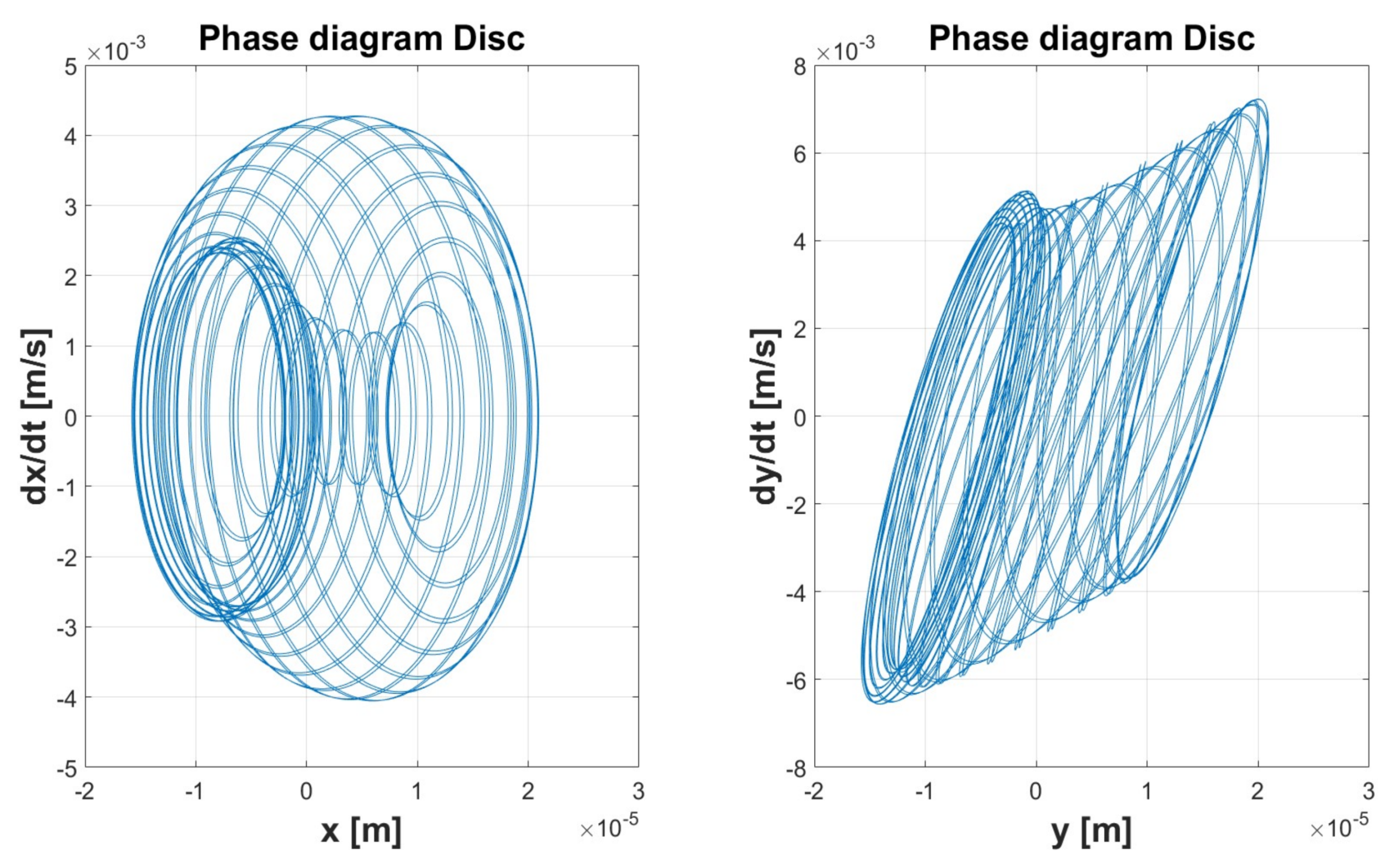

Figure 29.
Simulation 4: Cavitated—Normalized Power Spectrum.
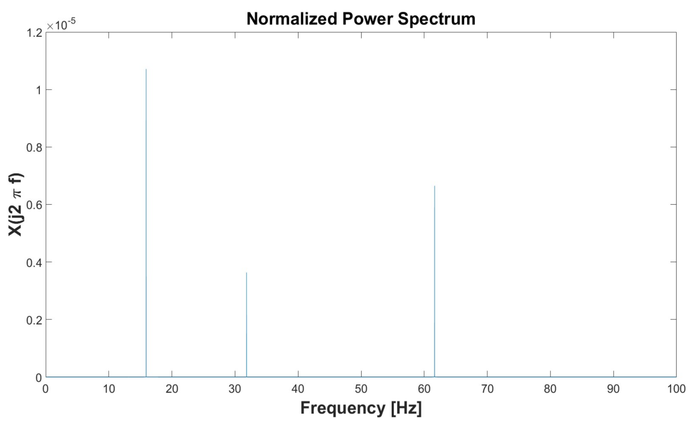
Figure 30.
Simulation 5: Uncavitated—Orbits.

Figure 31.
Simulation 5: Uncavitated—Phase Diagrams.
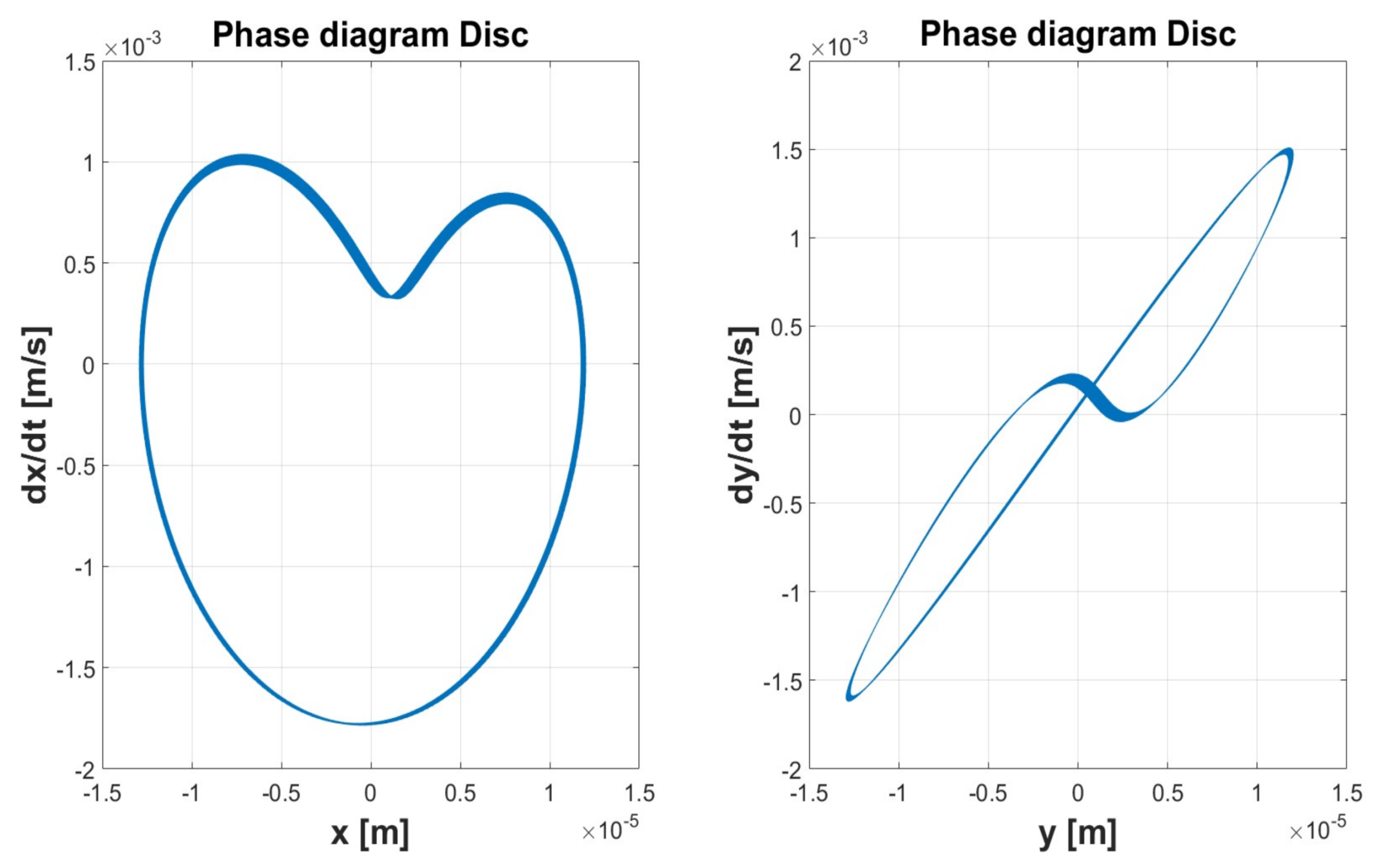
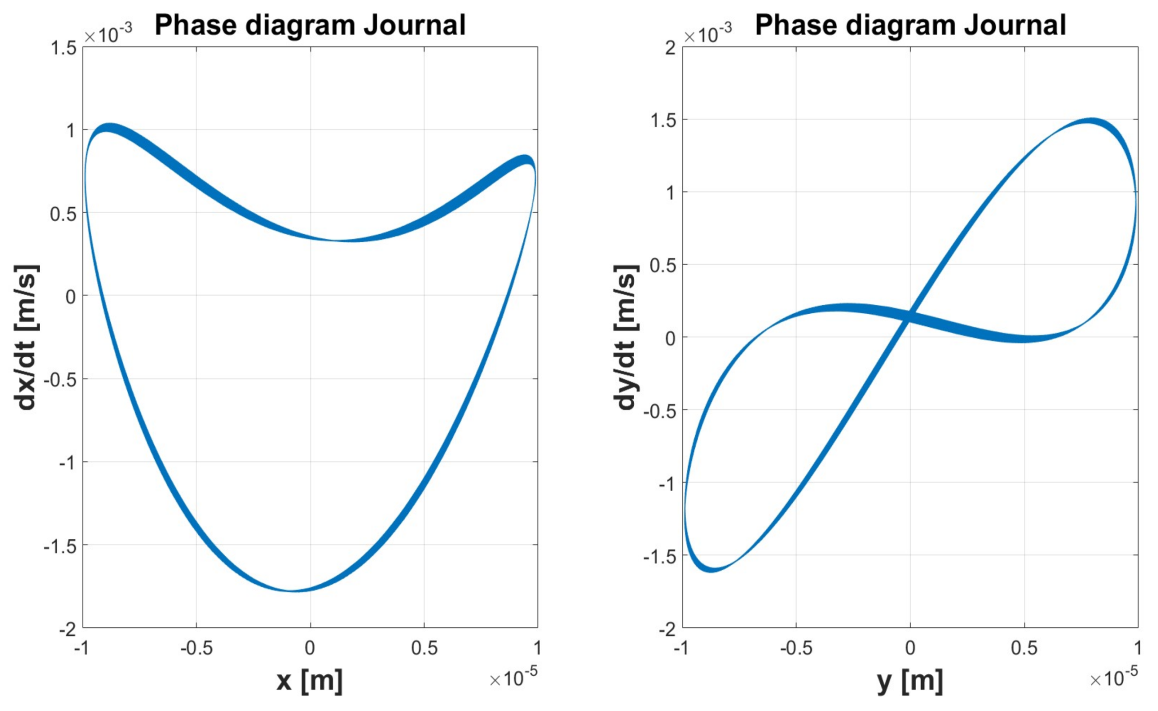
Figure 32.
Simulation 5: Uncavitated—Normalized Power Spectrum.

Figure 33.
Simulation 5: Cavitated—Orbits.


Figure 34.
Simulation 5: Cavitated—Phase Diagrams.
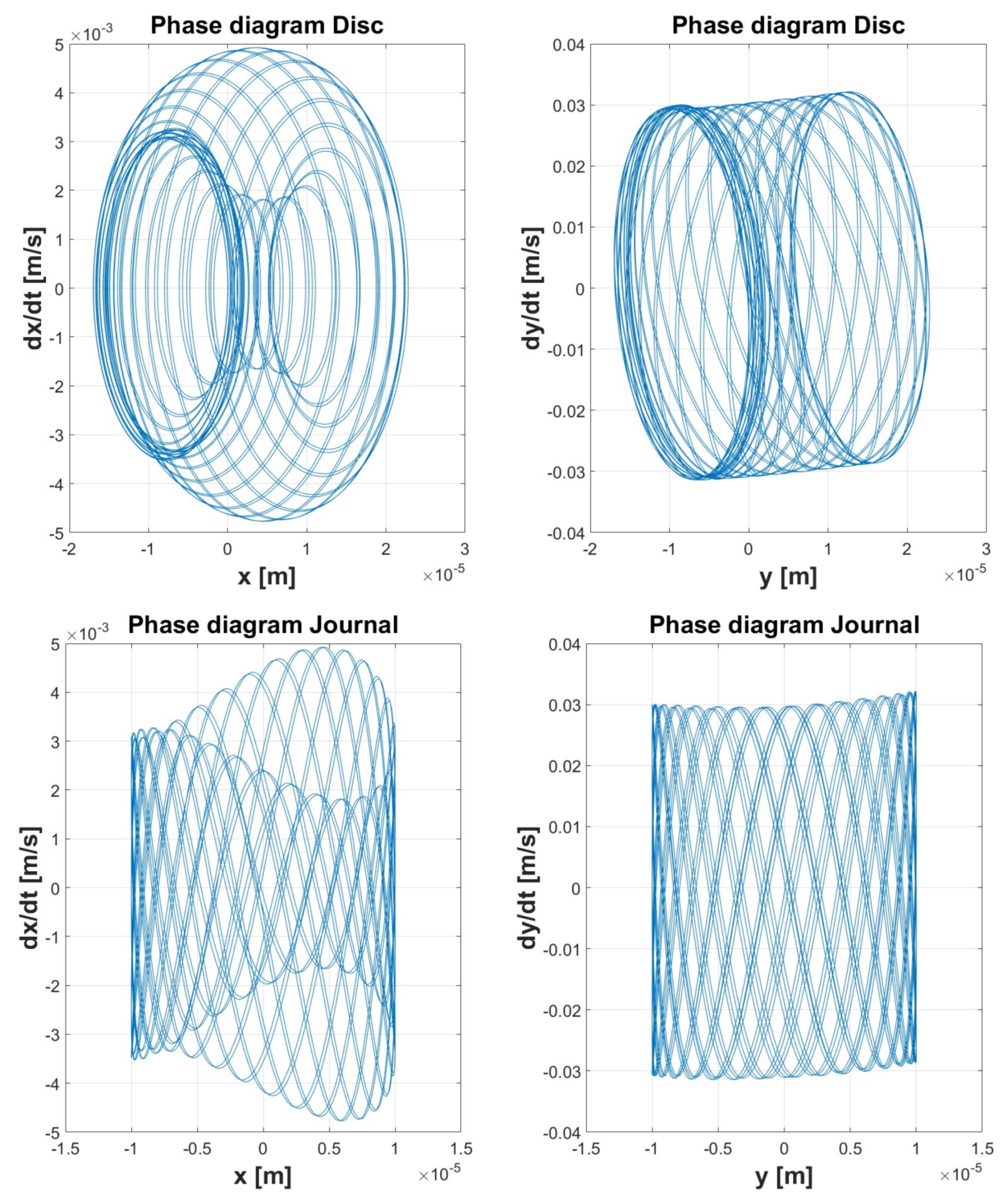
Figure 35.
Simulation 5: Cavitated—Normalized Power Spectrum.


Table 1.
Simulation parameters and initial condition for the Uncavitated Short Bearing and for the Cavitated (π-Film) Short Bearing.
Table 1.
Simulation parameters and initial condition for the Uncavitated Short Bearing and for the Cavitated (π-Film) Short Bearing.
| Simulation 1 | Simulation 2 | Simulation 3 | Simulation 4 | Simulation 5 | ||
|---|---|---|---|---|---|---|
| m (kg) | 10 | 1.5 | 5 × 101 | 2 | 2 | |
| K (N/m) | 106 | 4 × 10⁶ | 107 | 3 × 10⁵ | 3 × 10⁵ | |
| u (m) | 10−4 | 10−3 | 10−5 | 10−5 | 10−5 | |
| R (m) | 5 × 10⁻² | 1.6 × 10⁻² | 2 × 10⁻² | 5 × 10⁻³ | 5 × 10⁻³ | |
| L (m) | 5 × 10⁻² | 1.6 × 10⁻² | 2 × 10⁻² | 5 × 10⁻³ | 5 × 10⁻³ | |
| μ (kg/s) | 2 × 10⁻² | 3.4 × 10⁻² | 2.5 × 10⁻² | 2 × 10⁻² | 2 × 10⁻² | |
| ω (Hz) | 50 | 100 | 15.92 | 31.83 | 31.83 | |
| c (m) | 10−4 | 3.16 × 10⁻⁵ | 3.16 × 10⁻⁵ | 10−5 | 10−5 | |
| p0 (bar) | 2 | 2 | 2 | 2 | 2 | |
| 0 | 0 | 0 | 0 | 10−5 | ||
| 0 | 0 | 0 | 0 | 0 | ||
| −10−5 | −10−5 | −5 × 10⁻⁶ | −6 × 10⁻⁵ | 10−5 | ||
| 0 | 0 | 0 | 0 | 0 | ||
| 0 | 0 | 0 | 0 | 10−6 | ||
| −10−5 | −10−6 | −10−6 | −10−6 | 10−6 | ||
| Time | Uncavitated | 103 | 103 | 103 | 3 × 10³ | 3 × 10³ |
| Cavitated (π−Film) | 5 × 10² | 3 × 10³ | 3 × 10³ | 2 × 10³ | 2 × 10³ | |
| Solver | Ode4 | |||||
| Fixed-step size [s] | Uncavitated | 10−4 | 10−4 | 10−3 | 10−3 | 10−3 |
| Cavitated (π−Film) | 10−4 | 10−3 | 10−4 | 10−4 | 10−4 | |
© 2018 by the authors. Licensee MDPI, Basel, Switzerland. This article is an open access article distributed under the terms and conditions of the Creative Commons Attribution (CC BY) license (http://creativecommons.org/licenses/by/4.0/).
Share and Cite
MDPI and ACS Style
Ruggiero, A.; D’Amato, R.; Magliano, E.; Kozak, D. Dynamical Simulations of a Flexible Rotor in Cylindrical Uncavitated and Cavitated Lubricated Journal Bearings. Lubricants 2018, 6, 40. https://doi.org/10.3390/lubricants6020040
AMA Style
Ruggiero A, D’Amato R, Magliano E, Kozak D. Dynamical Simulations of a Flexible Rotor in Cylindrical Uncavitated and Cavitated Lubricated Journal Bearings. Lubricants. 2018; 6(2):40. https://doi.org/10.3390/lubricants6020040
Chicago/Turabian StyleRuggiero, Alessandro, Roberto D’Amato, Emanuele Magliano, and Drazan Kozak. 2018. "Dynamical Simulations of a Flexible Rotor in Cylindrical Uncavitated and Cavitated Lubricated Journal Bearings" Lubricants 6, no. 2: 40. https://doi.org/10.3390/lubricants6020040
Note that from the first issue of 2016, this journal uses article numbers instead of page numbers. See further details here.