Numerical Predictions of the Occurrence of Necking in Deep Drawing Processes


LEM3, UMR CNRS 7239—Arts et Métiers ParisTech, 4, rue Augustin Fresnel, 57078 Metz CEDEX 03, France
*
Author to whom correspondence should be addressed.
Metals 2017, 7(11), 455; https://doi.org/10.3390/met7110455
Submission received: 8 September 2017
/
Revised: 22 October 2017
/
Accepted: 23 October 2017
/
Published: 27 October 2017
(This article belongs to the Special Issue Advances in Plastic Forming of Metals)
Abstract
:In this work, three numerical necking criteria based on finite element (FE) simulations are proposed for the prediction of forming limit diagrams (FLDs) for sheet metals. An elastic–plastic constitutive model coupled with the Lemaitre continuum damage theory has been implemented into the ABAQUS/Explicit software to simulate simple sheet stretching tests as well as Erichsen deep drawing tests with various sheet specimen geometries. Three numerical criteria have been investigated in order to establish an appropriate necking criterion for the prediction of formability limits. The first numerical criterion is based on the analysis of the thickness strain evolution in the central part of the specimens. The second numerical criterion is based on the analysis of the second time derivative of the thickness strain. As to the third numerical criterion, it relies on a damage threshold associated with the occurrence of necking. The FLDs thus predicted by numerical simulation of simple sheet stretching with various specimen geometries and Erichsen deep drawing tests are compared with the experimental results.
Keywords:
modeling; simulation; sheet metal; necking; damage; forming limit diagrams; deep drawing test1. Introduction
The formability of sheet metals is usually characterized by forming limit diagrams (FLDs) obtained by the Nakazima or Marciniak deep drawing tests. The concept of FLD was first introduced by Keeler and Backofen [1] and subsequently improved by Goodwin [2]. The FLD is a limiting curve that depicts the in-plane major and minor strains of the sheet at the onset of localized necking, which precedes the final fracture. The FLD determination was originally based on experimental measurements, which turned out to be difficult and time-consuming. To overcome these drawbacks, a number of alternative theoretical and numerical approaches have been developed in the literature for the prediction of FLDs. These approaches are based on the combination of necking criteria with constitutive models for the prediction of necking in sheet metals. Among the theoretical necking criteria that have been developed in the literature for the prediction of necking, Swift [3] proposed an extension to biaxial stretching to the Considère maximum load criterion [4], which was utilized to predict diffuse necking in the expansion domain of the FLD. For localized necking, Hill [5] proposed an alternative criterion based on the bifurcation theory, which states that localized necking occurs along the direction of zero extension. It is worth noting that Hill’s criterion is only applicable to the left-hand side of the FLD and, therefore, it was often combined with the Swift criterion to determine a complete FLD. Marciniak and Kuczynski [6] developed another approach for localized necking prediction, which is known as the M–K criterion. The latter is based on the introduction of an initial imperfection, which ultimately triggers the occurrence of localized necking.
Concurrently with the above theoretical criteria, several numerical criteria for the prediction of necking and ductile fracture in sheet metals have been developed in the last few decades. Thanks to the growing progress in computational resources, simulation of complex sheet metal forming processes, such as the Nakazima and Marciniak deep drawing tests, using the finite element method (FEM) has become an interesting alternative to the theoretical approaches. Indeed, the substantial amount of results provided by FEM allows a realistic prediction of necking and fracture as compared to experiments. Using the FEM approach, the evolution of strain fields during loading is analyzed for each finite element within the sheet to detect the onset of necking. Burn et al. [7] analyzed the thinning of sheet metals, by using the Nakazima deep drawing test, in order to predict the onset of necking. Based on the Marciniak deep drawing test, Petek et al. [8] proposed a numerical approach for the prediction of necking, which consists in analyzing the time evolution of thickness strain and its first and second time derivatives. Later, Situ et al. [9,10,11] applied the same strategy to the Nakazima deep drawing test in order to predict FLDs for sheet metals involving the whole range of strain paths. They have shown that the analysis based on major strain rate (i.e., first time derivative of major strain) predicts the onset of fracture, while the maximum of major strain acceleration (i.e., second time derivative of major strain) corresponds to the occurrence of localized necking. Furthermore, another class of numerical criteria for the prediction of ductile fracture has emerged (see, e.g., [12,13,14,15,16]). These numerical criteria are based on empirical relationships, which depend on the application, and require several parameter calibrations with respect to experiments. They are labeled “fracture criteria”, as the associated FLDs are higher than those predicted using necking criteria.
The above numerical approaches for the prediction of necking and fracture are often combined with undamaged elastic–plastic constitutive models, which is not realistic from an experimental point of view. Indeed, the softening regime exhibited by the material behavior prior to fracture cannot be reproduced by elastic–plastic models alone, which requires the coupling of the constitutive equations with damage for a proper description of the material degradation and, thus, reliable prediction of final fracture. In this context, two well-established theories of ductile damage have been developed over the past few decades. The first theory is based on a micromechanical analysis of void growth, which describes the ductile damage mechanisms in porous materials. It was initiated by Gurson [17], modified by Tvergaard and Needleman [18], and subsequently improved by a number of contributors (see, e.g., [19,20,21,22]). The second theory, known as continuum damage mechanics (see, e.g., [23,24]), is based on the introduction of a damage variable, which represents the surface density of defects, and can be modeled as isotropic scalar variable (see, e.g., [23,25]), or tensor variable for anisotropic damage (see, e.g., [26,27,28]).
In this work, numerical necking criteria, based on finite element (FE) simulations, are proposed for the prediction of forming limit diagram for a steel material. The material response is described by an elastic–plastic model coupled with the Lemaitre isotropic damage approach [23]. The resulting constitutive equations have been implemented into the ABAQUS/Explicit code, within the framework of large strain and a three-dimensional formulation. Several specimen geometries have been simulated in order to reproduce all of the strain paths that are typically encountered in sheet metal forming processes. Two different FE models are considered to predict the FLDs of the studied material. First, the FLDs are predicted using simple sheet stretching tests, applied to different specimen geometries, in which no contact with tools is considered. Then, the FE model based on the Erichsen deep drawing test (see, e.g., [29]) is used to predict the FLDs of the steel material. To determine these forming limit curves for the studied material, three numerical criteria are presented in this work to detect the occurrence of necking in the sheet specimens. In the first numerical criterion, necking is detected when a sudden change in the evolution of the thickness strain at the central area of the specimen is observed. The second numerical criterion is based on the evolution of the thickness strain acceleration, which is obtained by computing the second time derivative of the thickness strain. As to the third numerical criterion, it relies on a critical damage threshold, at which is associated the occurrence of necking. All points of the predicted FLDs, which are obtained using the FE simulations combined with the numerical necking criteria, are compared with the experimental results taken from [30].
2. Constitutive Equations of the Ductile Damage Model
In this section, the elastic–plastic behavior law coupled with a ductile damage model is briefly presented. The latter is based on the continuum damage mechanics and, more specifically, on the Lemaitre isotropic damage model [23]. Using the concept of effective stress , and the strain equivalence principle, the continuum damage is introduced via the scalar variable by the following expression:
where is the Cauchy stress tensor, is the fourth-order elasticity tensor, and is the elastic strain tensor. The plastic yield function is written in the following form:
where is the equivalent stress, and is the deviatoric part of the effective stress. The fourth-order tensor contains the six anisotropy coefficients of the Hill quadratic yield criterion [31]. The isotropic hardening of the material is described by the size of the yield surface, while kinematic hardening is represented by the back-stress tensor .
The plastic flow rule is given by the normality law, which defines the plastic strain rate as
where is the plastic multiplier, and is the flow direction, normal to the yield surface in the stress space. With a special choice of co-rotational frame, which is associated with the Jaumann objective derivative, the Cauchy stress rate is written in the following form:
The evolution law for the damage variable is expressed by the following equation:
where is the strain energy density release rate (see, e.g., [25,32]), and , , and are four damage parameters that need to be identified. The expression of the strain energy density release rate is given (for linear isotropic elasticity) as follows:
where is the von Mises equivalent effective stress, is the hydrostatic effective stress (with being the second-order identity tensor), while and are, respectively, the Young’s modulus and Poisson’s ratio.
The above constitutive equations are implemented into the finite element code ABAQUS/Explicit using a co-rotational frame. The fourth-order Runge–Kutta explicit time integration scheme is used to update the stress state and all internal variables.
3. Numerical Integration of the Model and Its Validation
3.1. Time Integration Scheme
A user-defined material (VUMAT) subroutine is used for the implementation of the above elastic–plastic–damage model into the commercial finite element code ABAQUS/Explicit (Dassault Systèmes, France). For each integration point of the FE model, the stress state and all internal variables of the fully coupled elastic–plastic–damage model are known at the beginning of the loading increment. These stress state and internal variables will be updated through the VUMAT subroutine at the end of the loading increment. In this work, the fourth-order Runge–Kutta explicit time integration scheme is adopted to determine the updated stress state and all internal variables at the end of each loading increment. This straightforward integration algorithm represents a reasonable compromise in terms of computational efficiency, accuracy and convergence. Indeed, explicit time integration does not involve matrix inversion or iterative procedures for convergence, unlike implicit time integration. However, for explicit schemes, the time increment must be kept small enough to ensure accuracy and stability (see, e.g., [33,34]).
The evolution equations of the fully coupled model, which were presented in the previous section, can easily be written in the following compact form of general differential equation:
where vector encompasses all of the internal variables and stress state, while vector includes all evolution laws described in the previous section. The above condensed differential equation is then integrated over each loading increment, using the forward fourth-order Runge–Kutta explicit time integration scheme. The resulting algorithm is implemented into the finite element code ABAQUS/Explicit, via a VUMAT user-defined material subroutine, within the framework of large strains and a fully three-dimensional formulation.
3.2. Numerical Validation
In this section, the implementation of the fully coupled elastic–plastic–damage model described in the previous sections is validated through simulations of uniaxial tensile tests, which are then compared with reference solutions taken from the literature.
The first numerical example is a simple tensile test, which allows for the numerical validation of the elastic–plastic implementation of the model, without taking into account the damage contribution. For this purpose, the undamaged elastic–plastic model is recovered by setting to zero all the damage parameters. In this test, the von Mises yield surface is considered along with the Ludwig isotropic hardening law, which is defined by the following expression:
where represents the size of the yield surface, and is the equivalent plastic strain. In Equation (8), is the initial yield stress, while and are hardening parameters. Three standard steel materials, with three different values for the hardening exponent (see Equation (8)), are considered for the simulation of the uniaxial tensile test. The associated elastic–plastic material parameters are summarized in Table 1.
Figure 1 shows the uniaxial stress–strain curves obtained with the elastic–plastic model implemented in the VUMAT subroutine, which are compared with the numerical results given by the built-in elastic–plastic model available in ABAQUS. From these results, one can observe that the uniaxial stress–strain curves given by the VUMAT subroutine coincide with those provided by the built-in ABAQUS model, which demonstrates the successful implementation of the proposed model.
The second numerical test is intended to the validation of the proposed model when the damage behavior is taken into account. To this end, a uniaxial tensile test is simulated, according to the works of Doghri and Billardon [35], where a phenomenological elastic–plastic model with a von Mises plastic yield surface and Ludwig’s isotropic hardening is coupled with the Lemaitre damage approach. The studied materials are the same as those used in the previous test (see Table 1 for the elastic and hardening parameters), while the damage parameters used in the simulations are the same for the three materials, and are summarized in Table 2 (see [35]).
Figure 2 compares the stress–strain responses and the damage evolution obtained by the implemented fully coupled model with the reference solutions taken from [35]. It can be clearly observed that the simulated stress–strain curves and damage evolution coincide with their counterparts taken from the reference solutions, for the three materials investigated, which validates again the numerical implementation of the present elastic–plastic–damage model.
4. Identification of the St14 Steel Material Parameters
In this work, we investigate the occurrence of necking in a St14 steel material using the elastic–plastic–damage model described above in conjunction with numerical necking criteria. The mechanical behavior of the St14 steel is based on the Ludwig isotropic hardening law (see Equation (8)) and the von Mises yield surface, which are coupled with the Lemaitre isotropic damage approach. Standard tensile test experiments were performed by Aboutalebi et al. [36] for the investigated St14 steel. The corresponding experimental load–displacement curve is exploited in this work to identify the hardening and damage parameters for the studied St14 steel.
The hardening parameters of the Ludwig isotropic hardening law are first identified in the range of uniform elongation of the uniaxial tensile test. In this range of small to moderate deformations, where the stress and strain fields in the central region of the specimen remain homogeneous, the hardening parameters are accurately identified using a simple regression of the experimental data with the Ludwig power-law. The corresponding elastic and hardening material parameters are summarized in Table 3.
Then, the above-identified elastic–plastic parameters are used for the simulation of the uniaxial tensile test until the final fracture of the specimen. The damage parameters of the Lemaitre model are identified based on the entire experimental load–displacement response of the tensile test using an inverse identification procedure. The latter is based on least-squares minimization of the difference between the experimental and numerical load–displacement response for the uniaxial tensile test. The corresponding identified values for the Lemaitre damage model are summarized in Table 4.
Figure 3 compares the simulated load–displacement response, obtained using the identified material parameters of the Lemaitre damage model, with the experimental counterpart provided by Aboutalebi et al. [36]. This figure clearly shows that the simulated response using the present damage model is in very good agreement with the experimental curve and, in particular, demonstrates the ability of the implemented model to reproduce the sudden load drop that precedes the final fracture.
5. Description of the Finite Element Models
5.1. Finite Element Simulations
In this work, the predictions of the FLDs for the St14 steel material are carried out using the above elastic–plastic behavior model coupled with ductile damage. The numerical simulations are performed with the ABAQUS/explicit code. Ten specimens of the St14 sheet material with different geometries (a length of 120 mm, and a width varying from 12 mm to 120 mm, with a 12 mm increment in the width direction) are used in the simulations. Each specimen reproduces a particular strain path, which is typically encountered in sheet metal forming processes, and these strain paths range from uniaxial tension to equibiaxial expansion.
Two FE models are used for predicting the FLDs of the studied material. First, simple sheet stretching simulations, based on the different specimens, are performed. Then, the simulation of the deep drawing process, according to the Erichsen test (see, e.g., [29,30]), is conducted with the same specimens described above.
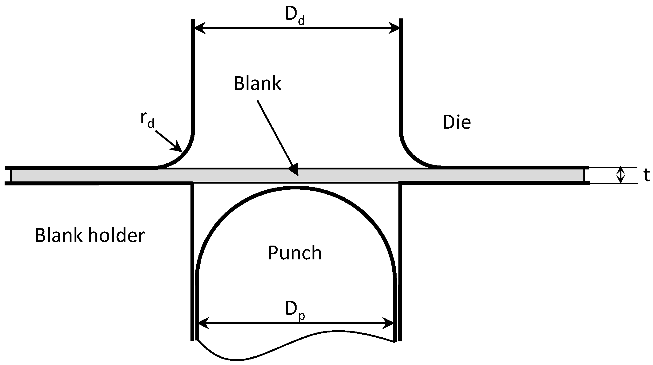
The schematic view of the Erichsen deep drawing test is illustrated in Figure 4.
The geometric parameters used in the simulations are (see [37]):
- Punch diameter Dp = 60 mm;
- Initial sheet thickness t = 0.8 mm;
- Die radius rd = 3 mm;
- Die opening diameter Dd = 66 mm.
Due to the symmetry of the problem, only one quarter of the geometry is discretized for each specimen. Figure 5 provides an illustration of the finite element models for the simple sheet stretching test and the Erichsen deep drawing test. For the particular case of the simple sheet stretching test, two different types of boundary conditions are considered in the simulations in order to reproduce most of the strain paths encountered in the simulations of the Erichsen deep drawing test with the various specimen widths. The first type of boundary conditions corresponds to a simple uniaxial tension, and these boundary conditions are applied to the specimens having a width ranging from 12 mm to 60 mm (see Figure 5a for illustration on the specimen having a width of 12 mm). The second type of boundary conditions corresponds to a proportional biaxial tension, and these boundary conditions are applied to the specimens having a width ranging from 72 mm to 120 mm (see Figure 5b for illustration on the specimen having a width of 84 mm).
The forming tools for the Erichsen deep drawing test are modeled as discrete rigid bodies. The friction coefficient between the tools and the specimen is taken to be equal to 0.15 [30].
5.2. Mesh Sensitivity
For material behavior that exhibits damage-induced softening, it is well known that the numerical solution, and particularly the localization zone, is prone to mesh sensitivity when a local elastic–plastic–damage model is used, which is the case in this work (see, e.g., [18,38,39]). In this section, several finite element models are adopted for the simulation of the uniaxial tensile specimen and the Erichsen deep drawing test, using the specimen with 12 mm width, in order to analyze the mesh-sensitivity effects. In all of the simulations that follow, the specimens are modeled with the eight-node three-dimensional continuum finite element with reduced integration (C3D8R), which is available in the ABAQUS/Explicit software. This element has only one integration point, which means that by considering n layers of elements in the thickness direction, the sheet thickness will be modeled with a total of n integration points.
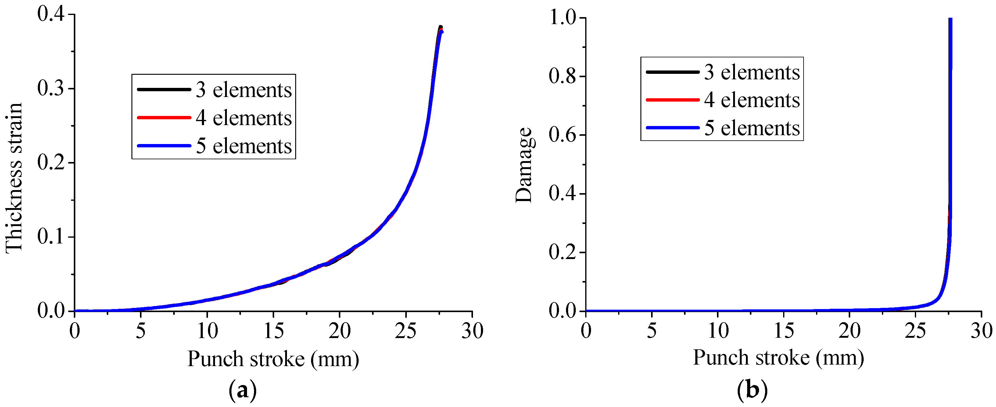
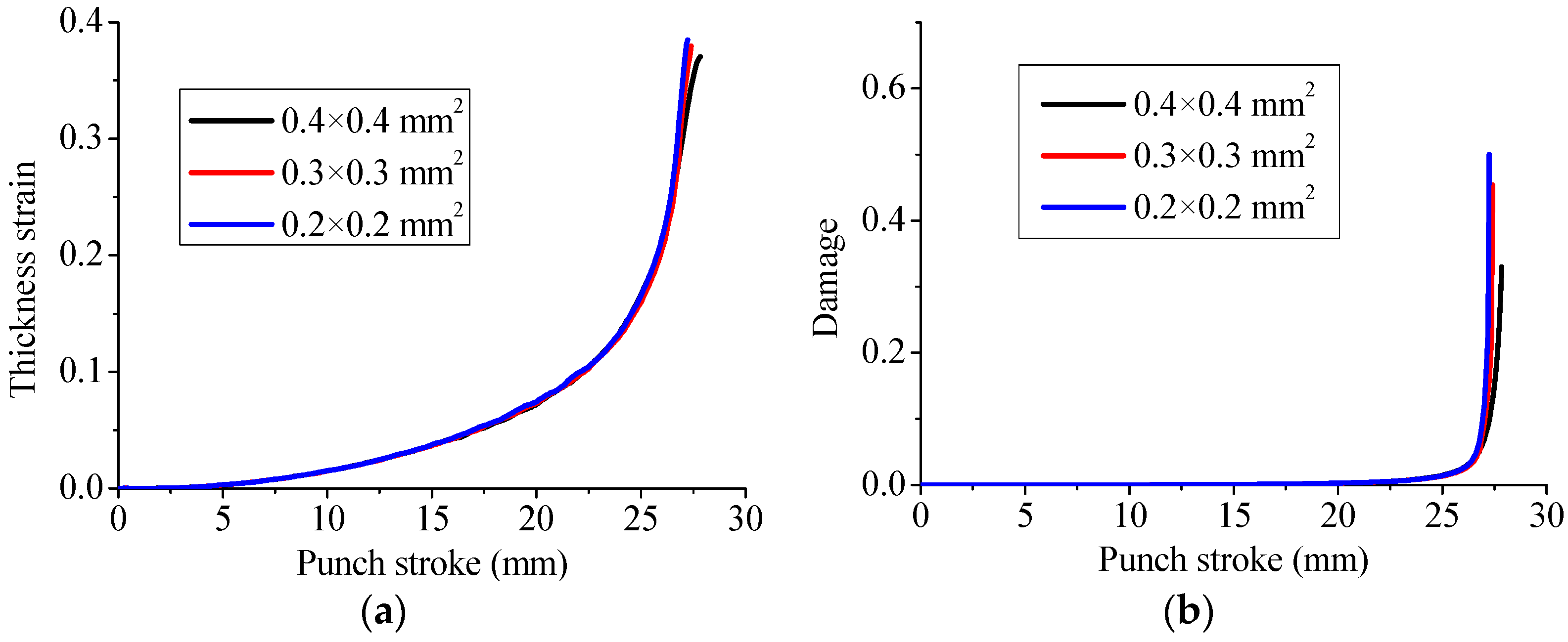
The effect of the number of elements in the thickness direction is first analyzed by considering, successively, three, then four, and finally five element layers through the thickness. In these three FE models, the same in-plane mesh is used to discretize the useful region of the specimen, with an intermediate in-plane element size of 0.3 × 0.3 mm2. Then, the impact of the in-plane FE discretization is analyzed by adopting for the useful region of the specimen four layers of elements through the thickness and three different in-plane element sizes (0.4 × 0.4 mm2, 0.3 × 0.3 mm2, and 0.2 × 0.2 mm2, respectively, as illustrated in Figure 6).
Figure 7 and Figure 8 reveal the influence of the number of elements in the thickness direction on the evolution of the thickness strain and the damage variable in the center of the specimen, as reflected by the simulation of the uniaxial tensile test and the Erichsen deep drawing test, respectively. It is clearly shown that only very small mesh dependence is observed, when varying the mesh refinement in the thickness direction, which suggests that four layers of elements are sufficient to describe the various nonlinear phenomena through the thickness.
Figure 9 and Figure 10 show the evolution of the thickness strain and damage variable in the center of the specimen, as determined by the present constitutive model with three different in-plane mesh sizes, for the uniaxial tensile test and Erichsen deep drawing test, respectively. In contrast to the results obtained with different numbers of element layers, the predicted thickness strain and damage variable reveal more sensitivity to in-plane mesh refinement when the damage variable becomes significant (i.e., ). More specifically, the numerical results obtained with the intermediate and finer meshes (0.3 × 0.3 mm2 and 0.2 × 0.2 mm2, respectively) are close to each other, which prompted us to use the in-plane mesh of 0.3 × 0.3 mm2 in the subsequent simulations. Indeed, this intermediate mesh involves reasonable computational times for all specimen geometries.
6. Numerical Criteria for the Prediction of the Occurrence of Necking
In this section, the numerical criteria used for the prediction of FLDs associated with the simple sheet stretching and the Erichsen simulations on various specimen geometries are presented. Three numerical criteria are adopted to predict the critical in-plane strains at the occurrence of necking. The first criterion is based on the analysis of the evolution of the thickness strain for each specimen. The occurrence of necking is detected when a sudden change in the evolution of the thickness strain in the central area is observed (see, e.g., [40]). The minor and major in-plane principal strains, corresponding to the occurrence of necking, are then reported into the FLD. To illustrate this procedure in the case of uniaxial tensile test, Figure 11 shows the evolution of the thickness strain in the central area of the specimen having a width of 12 mm. It is worth noting that, in the case of the Erichsen deep drawing test, the initiation of necking does not necessarily occur in the central area for all specimens. This feature, which depends on the specimen width and the contact between the punch and the specimen, is consistent with the experimental observations (see, e.g., [41]).
The second numerical criterion is based on the analysis of the thickness strain acceleration, which is obtained by computing the second time derivative of thickness strain in the central region of the specimen (see, e.g., [11,40,42]). According to this criterion, the critical minor and major in-plane principal strains at the occurrence of necking are obtained when the second time derivative of the thickness strain, i.e., thickness strain acceleration, reaches a maximum. This is illustrated in Figure 12 for the uniaxial tensile test corresponding to the specimen having a width of 12 mm. Note that the occurrence of localized necking may also be predicted using the first time derivative of thickness strain, which represents the thickness strain rate. However, several works in the literature have shown that the numerical criterion based on the maximum of strain acceleration is more appropriate for the prediction of localized necking than the one based on the maximum of strain rate, as the latter rather indicates the onset of fracture (see, e.g., [8,9]).
A third numerical criterion is analyzed in this work based on a critical damage threshold at which is associated the occurrence of necking. Unlike the numerical criteria described above, the same critical damage value is used here for all simulations using the various specimen geometries. This critical damage value was identified by Aboutalebi et al. [36] using the Vickers micro-hardness test. Using simple sheet stretching tests and Erichsen deep drawing tests, the simulations are performed until the critical damage value of 0.434 is reached at some finite element of the discretized model (see an illustration in Figure 13, in the case of uniaxial tensile test for the specimen with 12 mm width). At this instant, the simulations are stopped and the minor and major in-plane principal strains of the corresponding finite element are plotted into the FLD.
7. Application to the Determination of FLDs
The present numerical methodology, based on the three above-described numerical criteria, is applied in this section to both the simple sheet stretching and the Erichsen simulations with various specimen geometries in order to obtain complete FLDs for the studied material.
Once the simulations of the simple sheet stretching test and the Erichsen test performed for the various specimen geometries, the corresponding numerical load–displacement curves, which are obtained using the previously identified hardening and damage parameters, are plotted in Figure 14. It can be observed that, for both the simple sheet stretching test and the Erichsen test, the fully coupled model reproduces satisfactorily the peak in the load–displacement curves, which is followed by the sudden load drop caused by the damage acceleration at the latest stages of loading.
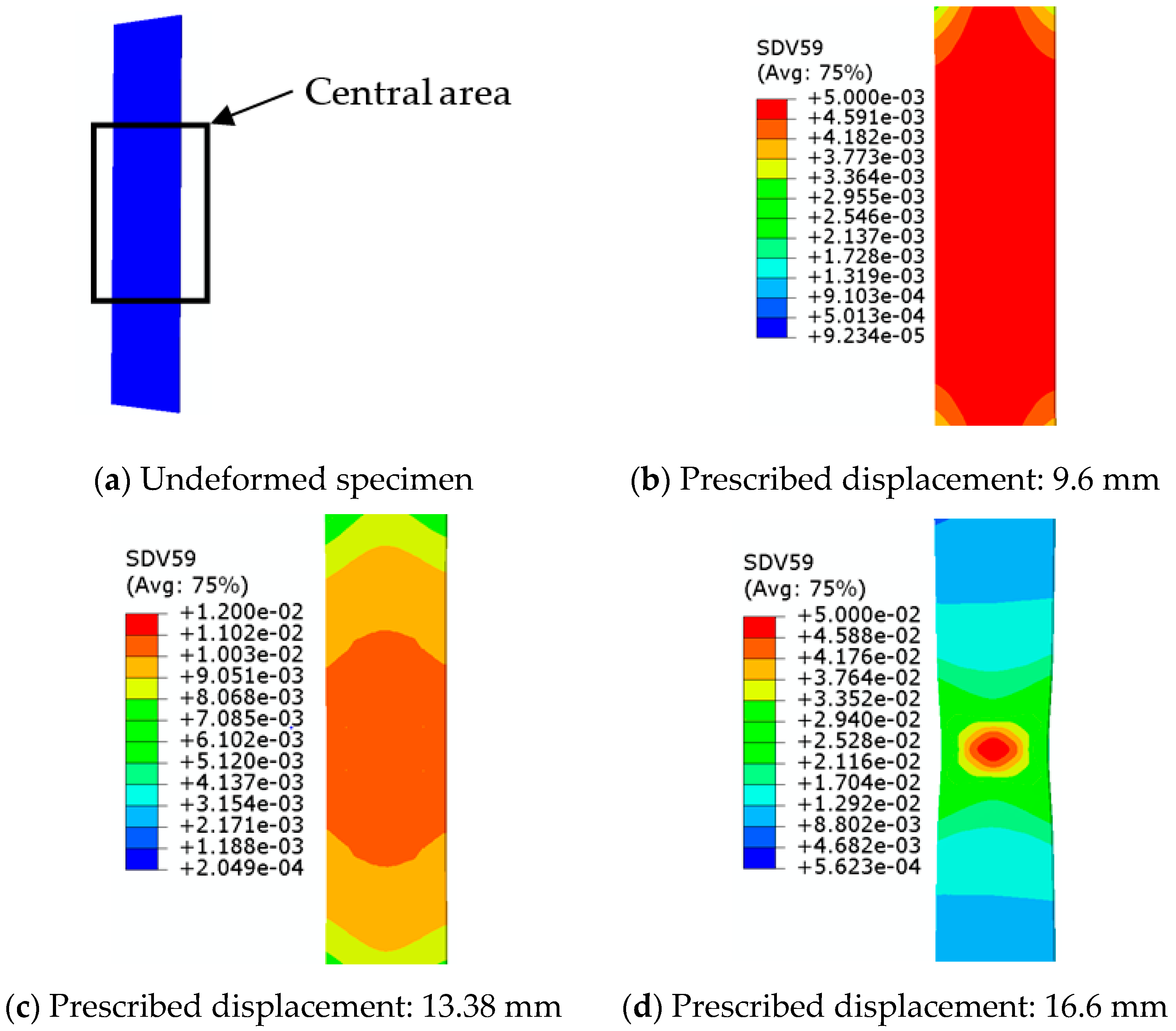
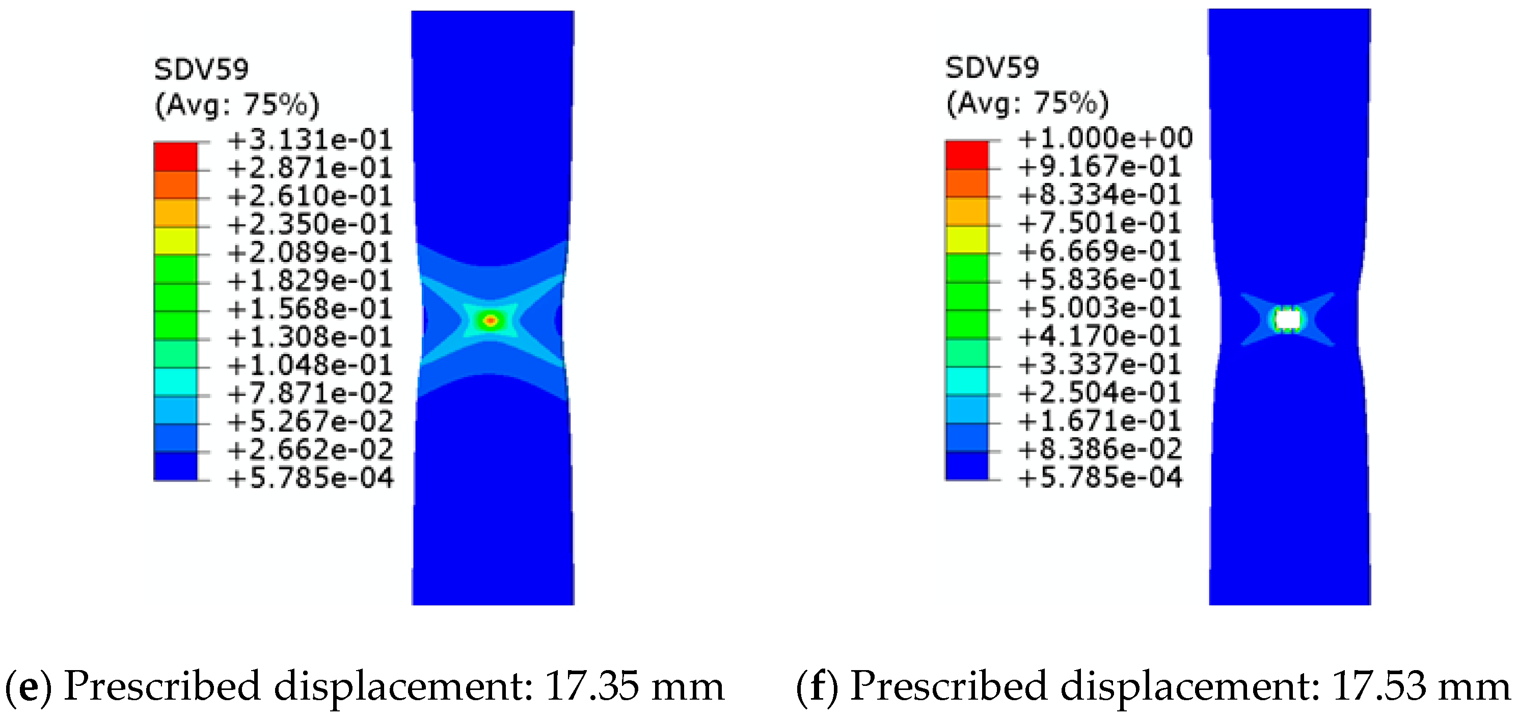
Moreover, Figure 15 and Figure 16 show the distribution of the damage variable, at different stages of loading, as determined by the numerical simulation of the simple sheet stretching test on the specimen having a width of 12 mm and the Erichsen test on the specimen having a width of 24 mm, respectively. More specifically, for the simple sheet stretching test (i.e., Figure 15), the damage distribution in the central part of the specimen remains uniform until the applied loading reaches its maximum (see Figure 14a). Beyond this limit, the damage distribution becomes heterogeneous, and concentrates gradually in the middle of the specimen in the form of two localization bands (Figure 15e). Finally, the accumulated damage in the narrow bands leads to highly localized necking, which ultimately results in a macrocrack (Figure 15f).
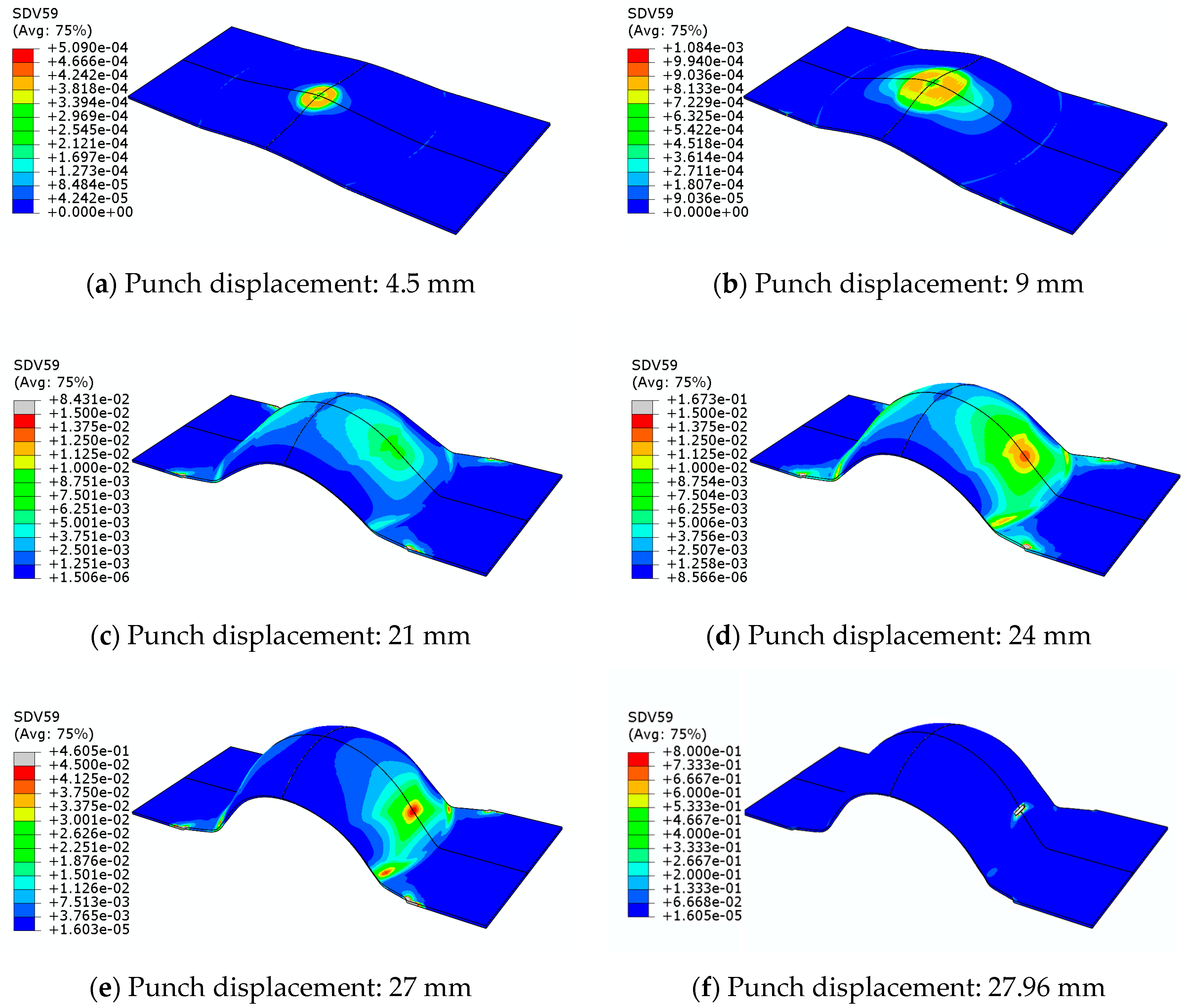
For the Erichsen deep drawing test, the damage distribution is localized around the dome apex of the specimen (i.e., higher specimen point) in the early stages of the deep drawing process, with low damage levels (i.e., , see Figure 16a,b). As the punch moves down, a strong localization of damage distribution is observed far from the dome apex, which is due to the frictional contact between the punch and the specimen (see Figure 16d,e). Finally, the damage accumulation leads to localized necking followed by fracture, as shown in Figure 16f.
The strain paths generated by the simulations of the simple sheet stretching test and the Erichsen test for all specimen widths are reported in Figure 17. Similar trends for the strain-path evolution are observed between both tests. More specifically, the strain paths are almost linear for the specimens having widths ranging from 12 mm to 60 mm (i.e., corresponding to a negative minor strain), while they are clearly nonlinear for the specimens having widths ranging from 72 mm to 120 mm (i.e., corresponding to a positive minor strain). In the latter case, the strain paths remain linear until a sudden transition to some plane-strain state, which indicates the onset of localized necking (see, e.g., [40,43]).
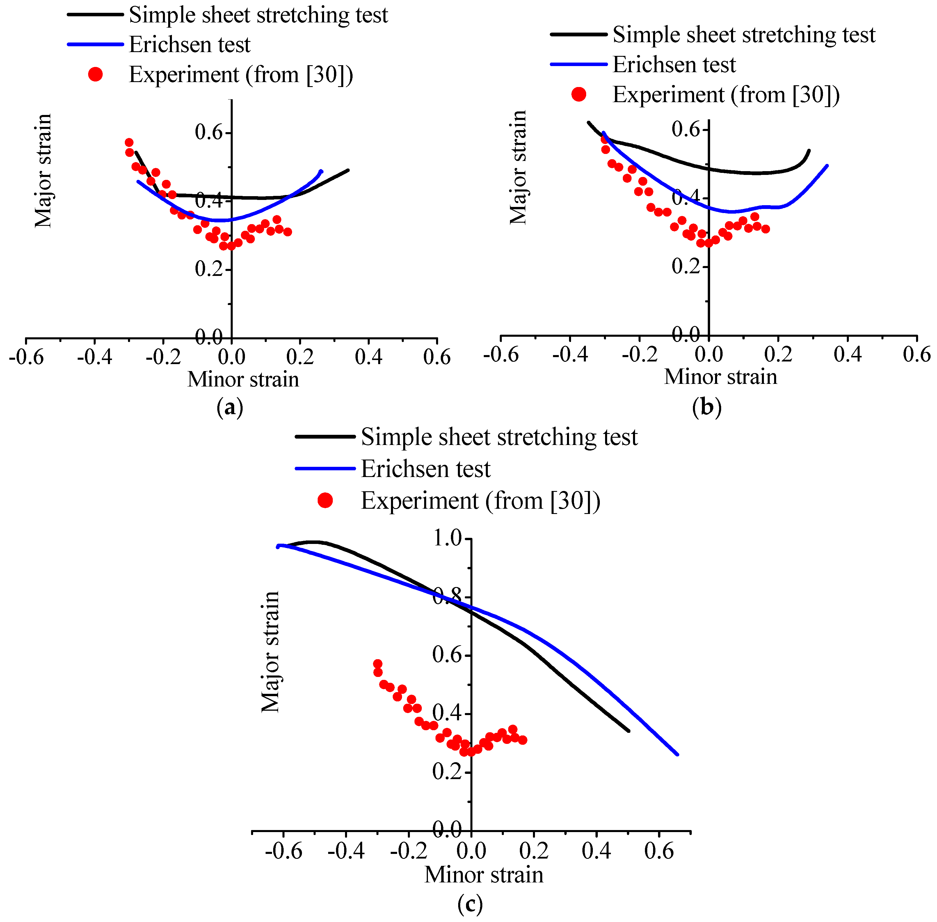
Figure 18 compares the predicted FLDs for the studied material, based on the simulations of both simple sheet stretching and Erichsen tests, along with the experimental results provided by Aboutalebi et al. [30]. The FLDs based on the analyses of thickness strain, second time derivative of thickness strain, and critical damage threshold are presented in Figure 18a–c, respectively.
Note that the experimental results given by Aboutalebi et al. [30] are obtained using the same Erichsen deep drawing test used in the simulations, which allows consistent comparison between the predicted FLDs and the experimental data. It can be noticed, in general, that the numerical predictions of the FLDs obtained by the Erichsen deep drawing tests are closer to the experimental results than those predicted by simple sheet stretching tests. The fact that the trends obtained by simulation of Erichsen deep drawing tests are more consistent with the experimental results may be explained by the similarity in the mechanical setups used in both cases (i.e., Erichsen deep drawing test), while no forming tools are considered in the simple sheet stretching tests. More specifically, in the left-hand side of the FLDs, the results predicted from Erichsen deep drawing tests using the numerical criteria based on the thickness strain evolution and the second time derivative of thickness strain are in reasonably good agreement with the experimental results, while the predictions overestimate the occurrence of necking when they are based on the critical damage threshold criterion.
In the right-hand side of the FLDs (i.e., positive minor strains), the results predicted from the Erichsen deep drawing tests using the numerical criterion based on the second time derivative of thickness strain show the best agreement with respect to experiments (see Figure 18b). Note that the FLDs predicted from both Erichsen deep drawing tests and simple sheet stretching tests on the basis of the critical damage threshold criterion are overestimated for all strain paths, which proves that this numerical criterion is not suitable for the prediction of the occurrence of necking. Moreover, based on this critical damage threshold criterion, the shapes of the FLDs correspond rather to fracture limit diagrams, which are classically determined in the literature using numerical fracture criteria (see, e.g., [44]). The unsuitability of the latter numerical criterion may be explained by its consideration of a constant critical damage value for all strain paths, which is a strong assumption, since the damage value at the occurrence of necking depends on the stress triaxiality ratio and, therefore, on the loading path (see, e.g., [45]).
8. Conclusions
In this paper, an elastic–plastic model has been coupled with the Lemaitre ductile damage approach in order to predict the occurrence of necking in sheet metal forming. The whole set of coupled constitutive equations has been implemented into the finite element code ABAQUS/Explicit in the framework of large strains and a fully three-dimensional formulation. Three numerical necking criteria have been considered for predicting the occurrence of necking in sheet metals. They are based on the analyses of the local thickness strain evolution and its second time derivative during the FE simulations, as well as on a fixed critical damage threshold at which is associated the occurrence of necking. For the FE simulations, simple sheet stretching tests as well as Erichsen deep drawing tests on various specimen geometries, covering all possible strain paths, were used in conjunction with the numerical necking criteria. The numerical results in terms of FLDs were compared to the experimental results taken from [30]. Good agreement between the predicted FLD and the experiments was observed using the Erichsen deep drawing test combined with the numerical criterion based on the second time derivative of thickness strain. Due to the low cost and computational efficiency of the numerical alternative for FLD prediction, as compared to the lengthy and expensive experimental procedures, the proposed numerical approach can be easily used with different forming setups and a large variety of materials for the prediction of the occurrence of necking in sheet metals.
Author Contributions
Hocine Chalal conceived and performed the simulations. Hocine Chalal and Farid Abed-Meraim analyzed and discussed the results. Both authors contributed to the writing of the manuscript.
Conflicts of Interest
The authors declare no conflict of interest.
References
- Keeler, S.; Backofen, W.A. Plastic instability and fracture in sheets stretched over rigid punches. ASM Trans. Q. 1963, 56, 25–48. [Google Scholar]
- Goodwin, G. Application of strain analysis to sheet metal forming problems in the press shop. SAE Tech. Pap. 1968. [Google Scholar] [CrossRef]
- Swift, H.W. Plastic instability under plane stress. J. Mech. Phys. Solids 1952, 1, 1–18. [Google Scholar] [CrossRef]
- Considère, A. Mémoire sur l’emploi du fer et de l’acier dans les constructions. Annals Ponts Chaussées 1885, 9, 574. [Google Scholar]
- Hill, R. On discontinuous plastic states, with special reference to localized necking in thin sheets. J. Mech. Phys. Solids 1952, 1, 19–30. [Google Scholar] [CrossRef]
- Marciniak, Z.; Kuczyński, K. Limit strains in the processes of stretch-forming sheet metal. Int. J. Mech. Sci. 1967, 9, 609–620. [Google Scholar] [CrossRef]
- Brun, R.; Chambard, A.; Lai, M.; De Luca, P. Actual and virtual testing techniques for a numerical definition of materials. In Proceedings of the 4th International Conference and Workshop NUMISHEET ’99, Besançon, France, 13–17 September 1999; pp. 393–398. [Google Scholar]
- Petek, A.; Pepelnjak, T.; Kuzman, K. An improved method for determining forming limit diagram in the digital environment. J. Mech. Eng. 2005, 51, 330–345. [Google Scholar]
- Situ, Q.; Jain, M.K.; Bruhis, M. A suitable criterion for precise determination of incipient necking in sheet materials. Mater. Sci. Forum 2006, 519–521, 111–116. [Google Scholar] [CrossRef]
- Situ, Q.; Jain, M.K.; Bruhis, M. Further experimental verification of a proposed localized necking criterion. In Proceedings of the 9th International Conference on Numerical Methods in Industrial Forming Processes, Porto, Portugal, 17–21 June 2007; pp. 907–912. [Google Scholar]
- Situ, Q.; Jain, M.K.; Bruhis, M.; Metzger, D.R. Determination of forming limit diagrams of sheet materials with a hybrid experimental-numerical approach. Int. J. Mech. Sci. 2011, 53, 707–719. [Google Scholar] [CrossRef]
- Clift, S.E.; Hartley, P.; Sturgess, C.E.N.; Rowe, G.W. Fracture prediction in plastic deformation processes. Int. J. Mech. Sci. 1990, 32, 1–17. [Google Scholar] [CrossRef]
- Wierzbicki, T.; Bao, Y.; Lee, Y.-W.; Bai, Y. Calibration and evaluation of seven fracture models. Int. J. Mech. Sci. 2005, 47, 719–743. [Google Scholar] [CrossRef]
- Bao, Y.; Wierzbicki, T. On fracture locus in the equivalent strain and stress triaxiality space. Int. J. Mech. Sci. 2004, 46, 81–98. [Google Scholar] [CrossRef]
- Han, H.N.; Kim, K.-H. A ductile fracture criterion in sheet metal forming process. J. Mater. Process. Technol. 2003, 142, 231–238. [Google Scholar] [CrossRef]
- Jain, M.; Allin, J.; Lloyd, D.J. Fracture limit prediction using ductile fracture criteria for forming of an automotive aluminum sheet. Int. J. Mech. Sci. 1999, 41, 1273–1288. [Google Scholar] [CrossRef]
- Gurson, A.L. Continuum theory of ductile rupture by void nucleation and growth: Part I—Yield criteria and flow rules for porous ductile media. J. Eng. Mater. Technol. 1977, 99, 2–15. [Google Scholar] [CrossRef]
- Tvergaard, V.; Needleman, A. Analysis of the cup-cone fracture in a round tensile bar. Acta Metall. Mater. 1984, 32, 157–169. [Google Scholar] [CrossRef]
- Rousselier, G. Ductile fracture models and their potential in local approach of fracture. Nucl. Eng. Des. 1987, 105, 97–111. [Google Scholar] [CrossRef]
- Pardoen, T.; Doghri, I.; Delannay, F. Experimental and numerical comparison of void growth models and void coalescence criteria for the prediction of ductile fracture in copper bars. Acta Mater. 1998, 46, 541–552. [Google Scholar] [CrossRef]
- Benzerga, A.A.; Besson, J. Plastic potentials for anisotropic porous solids. Eur. J. Mech. A/Solids 2001, 20, 397–434. [Google Scholar] [CrossRef]
- Monchiet, V.; Cazacu, O.; Charkaluk, E.; Kondo, D. Macroscopic yield criteria for plastic anisotropic materials containing spheroidal voids. Int. J. Plast. 2008, 24, 1158–1189. [Google Scholar] [CrossRef]
- Lemaitre, J. A continuous damage mechanics model for ductile fracture. J. Eng. Mater. Technol. ASME 1985, 107, 83–89. [Google Scholar] [CrossRef]
- Chaboche, J.L. Thermodynamically founded CDM models for creep and other conditions. In Creep and Damage in Materials and Structures; CISM Courses and Lectures No 399, International Centre for Mechanical Sciences; Springer: Vienna, Austria, 1999; Volume 399, pp. 209–283. [Google Scholar]
- Lemaitre, J. A Course on Damage Mechanics; Springer: Berlin, Germany, 1992. [Google Scholar]
- Chow, C.L.; Lu, T.J. On evolution laws of anisotropic damage. Eng. Fract. Mech. 1989, 34, 679–701. [Google Scholar] [CrossRef]
- Chaboche, J.L. Development of continuum damage mechanics for elastic solids sustaining anisotropic and unilateral damage. Int. J. Damage Mech. 1993, 2, 311–329. [Google Scholar] [CrossRef]
- Abu Al-Rub, R.K.; Voyiadjis, G.Z. On the coupling of anisotropic damage and plasticity models for ductile materials. Int. J. Solids Struct. 2003, 40, 2611–2643. [Google Scholar] [CrossRef]
- Takuda, H.; Yoshii, T.; Hatta, N. Finite-element analysis of the formability of a magnesium-based alloy AZ31 sheet. J. Mater. Process. Technol. 1999, 89–90, 135–140. [Google Scholar] [CrossRef]
- Aboutalebi, F.H.; Farzin, M.; Mashayekhi, M. Numerical prediction and experimental validations of ductile damage evolution in sheet metal forming processes. Acta Mech. Solida Sin. 2012, 25, 638–650. [Google Scholar] [CrossRef]
- Hill, R. A theory of the yielding and plastic flow of anisotropic metals. Proc. R. Soc. A 1948, 193, 281–297. [Google Scholar] [CrossRef]
- Lemaitre, J.; Desmorat, R.; Sauzay, M. Anisotropic damage law of evolution. Eur. J. Mech. A Solids 2000, 9, 187–208. [Google Scholar] [CrossRef]
- Li, Y.-F.; Nemat-Nasser, S. An explicit integration scheme for finite deformation plasticity in finite-element methods. Finite Elem. Anal. Des. 1993, 15, 93–102. [Google Scholar] [CrossRef]
- Kojic, M. Stress integration procedures for inelastic material models within finite element method. ASME Appl. Mech. Rev. 2002, 55, 389–414. [Google Scholar] [CrossRef]
- Doghri, I.; Billardon, R. Investigation of localization due to damage in elasto-plastic materials. Mech. Mater. 1995, 19, 129–149. [Google Scholar] [CrossRef]
- Aboutalebi, F.H.; Farzin, M.; Poursina, M. Numerical simulation and experimental validation of a ductile damage model for DIN 1623 St14 steel. Int. J. Adv. Manuf. Technol. 2011, 53, 157–165. [Google Scholar] [CrossRef]
- Aboutalebi, F.H.; Banihashemi, A. Numerical estimation and practical validation of Hooputra’s ductile damage parameters. Int. J. Adv. Manuf. Technol. 2014, 75, 1701–1710. [Google Scholar] [CrossRef]
- Besson, J.; Steglich, D.; Brocks, W. Modeling of crack growth in round bars and plane strain specimens. Int. J. Solids Struct. 2001, 38, 8259–8284. [Google Scholar] [CrossRef]
- Peerlings, R.H.G.; Geers, M.G.D.; de Borst, R.; Brekelmans, W.A.M. A critical comparison of nonlocal and gradient-enhanced softening continua. Int. J. Solids Struct. 2001, 38, 7723–7746. [Google Scholar] [CrossRef]
- Zhang, C.; Leotoing, L.; Zhao, G.; Guines, D.; Ragneau, E. A comparative study of different necking criteria for numerical and experimental prediction of FLCs. J. Mater. Eng. Perform. 2011, 20, 1036–1042. [Google Scholar] [CrossRef]
- Kami, A.; Dariani, B.M.; Vanini, A.S.; Comsa, D.S.; Banabic, D. Numerical determination of the forming limit curves of anisotropic sheet metals using GTN damage model. J. Mater. Process. Technol. 2015, 216, 472–483. [Google Scholar] [CrossRef]
- Volk, W.; Hora, P. New algorithm for a robust user-independent evaluation of beginning instability for the experimental FLC determination. Int. J. Mater. Form. 2011, 4, 339–346. [Google Scholar] [CrossRef]
- Liewald, M.; Drotleff, K. Novel punch design for nonlinear strain path generation and evaluation methods. Key Eng. Mater. 2015, 639, 317–324. [Google Scholar] [CrossRef]
- Silva, M.B.; Martínez-Donaireb, A.J.; Centenob, G.; Morales-Palmab, D.; Vallellanob, C.; Martinsa, P.A.F. Recent approaches for the determination of forming limits by necking and fracture in sheet metal forming. Procedia Eng. 2015, 132, 342–349. [Google Scholar] [CrossRef]
- Soyarslan, C.; Richter, H.; Bargmann, S. Variants of Lemaitre’s damage model and their use in formability prediction of metallic materials. Mech. Mater. 2016, 92, 58–79. [Google Scholar] [CrossRef]
Figure 1.
Validation of the numerical implementation of the undamaged elastic–plastic model with respect to the built-in ABAQUS model.
Figure 1.
Validation of the numerical implementation of the undamaged elastic–plastic model with respect to the built-in ABAQUS model.
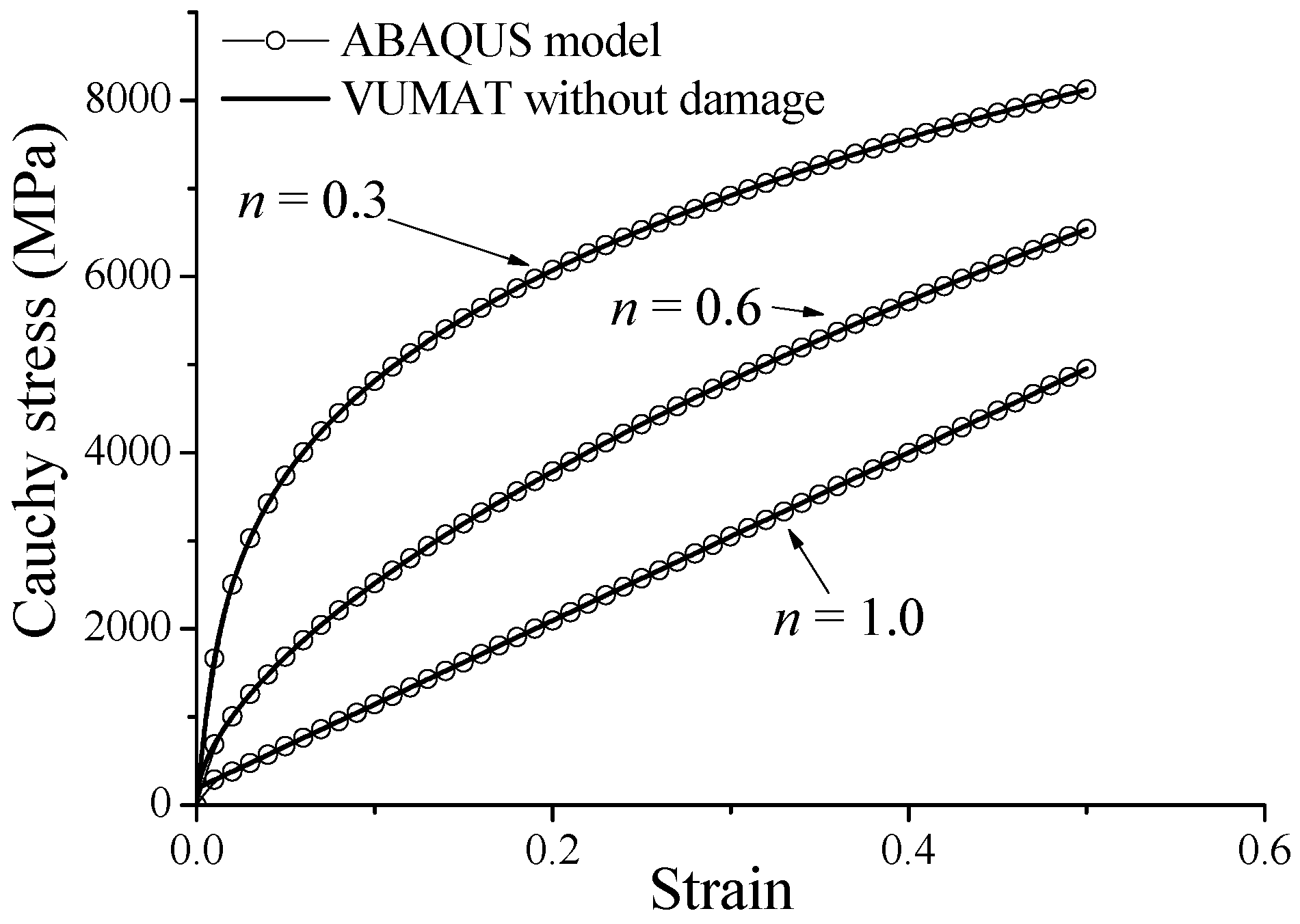
Figure 2.
Validation of the numerical implementation of the fully coupled elastic–plastic–damage model with respect to reference solutions taken from [35] for the three studied materials: (a) uniaxial tensile stress–strain curves; and (b) damage evolution.
Figure 2.
Validation of the numerical implementation of the fully coupled elastic–plastic–damage model with respect to reference solutions taken from [35] for the three studied materials: (a) uniaxial tensile stress–strain curves; and (b) damage evolution.
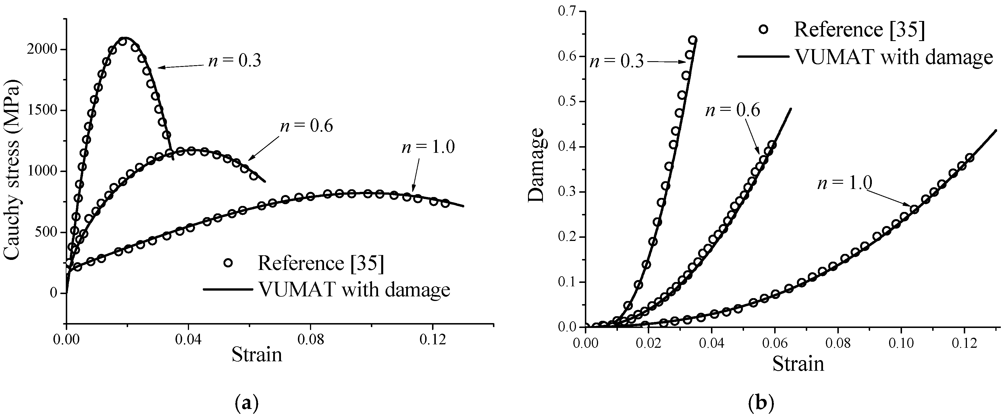
Figure 3.
Tensile load–displacement response simulated with the Lemaitre damage model, along with the experimental curve taken from Aboutalebi et al. [36].
Figure 3.
Tensile load–displacement response simulated with the Lemaitre damage model, along with the experimental curve taken from Aboutalebi et al. [36].
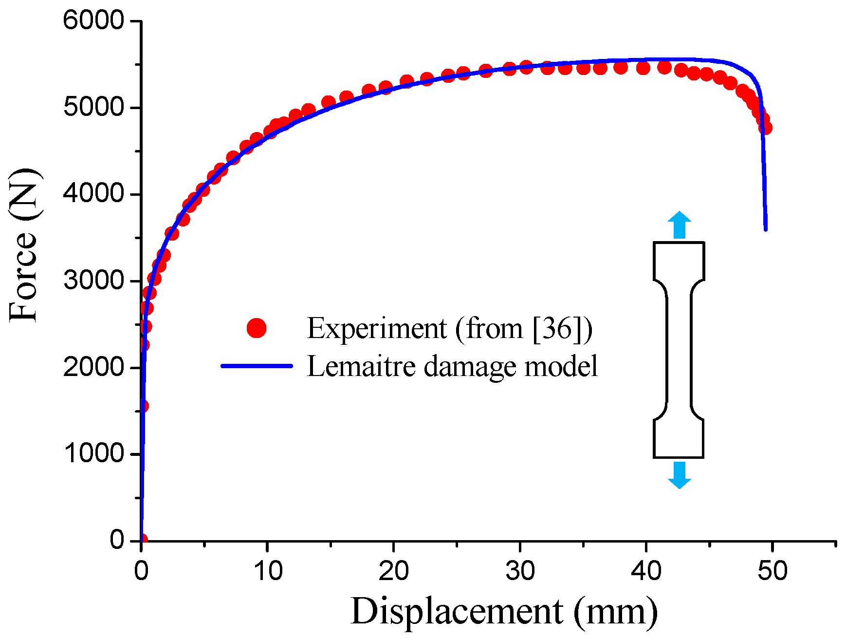
Figure 4.
Schematic view of the Erichsen deep drawing test.

Figure 5.
FE models corresponding to (a) uniaxial tensile test; (b) biaxial tensile test; and (c) Erichsen deep drawing test.
Figure 5.
FE models corresponding to (a) uniaxial tensile test; (b) biaxial tensile test; and (c) Erichsen deep drawing test.
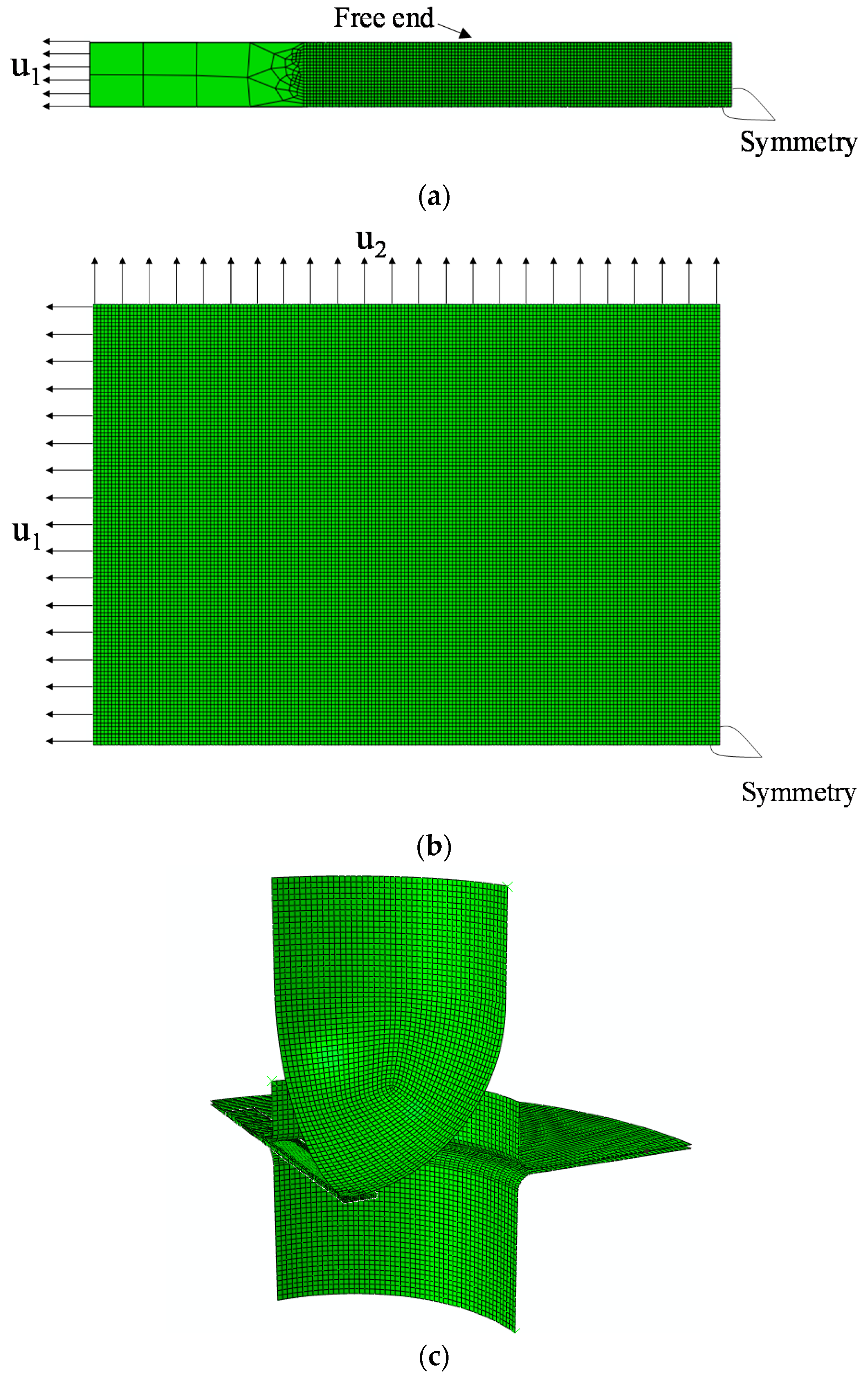
Figure 6.
In-plane FE discretization for the central region of the specimen: (a) 0.4 × 0.4 mm2; (b) 0.3 × 0.3 mm2; and (c) 0.2 × 0.2 mm2.
Figure 6.
In-plane FE discretization for the central region of the specimen: (a) 0.4 × 0.4 mm2; (b) 0.3 × 0.3 mm2; and (c) 0.2 × 0.2 mm2.
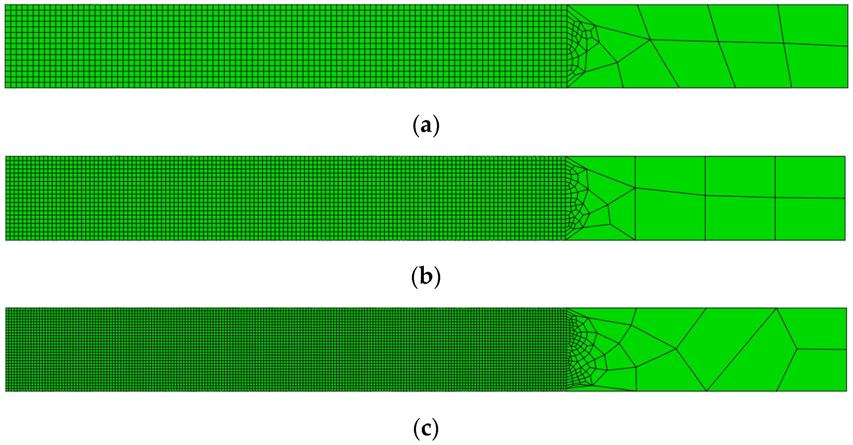
Figure 7.
Effect of the number of elements in the thickness direction on the evolution of (a) thickness strain and (b) damage, during the uniaxial tensile test for the specimen with 12 mm width.
Figure 7.
Effect of the number of elements in the thickness direction on the evolution of (a) thickness strain and (b) damage, during the uniaxial tensile test for the specimen with 12 mm width.
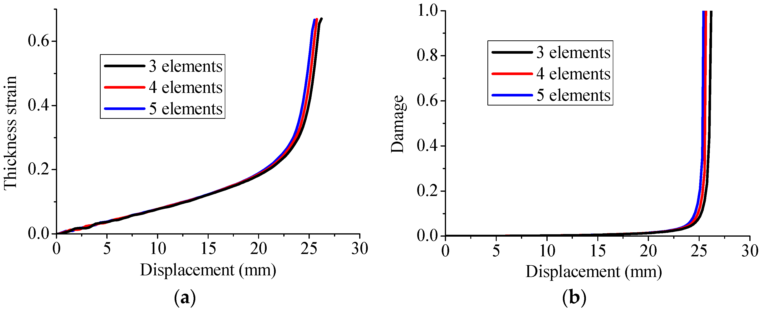
Figure 8.
Effect of the number of elements in the thickness direction on the evolution of (a) thickness strain and (b) damage, during the Erichsen deep drawing test for the specimen with 12 mm width.
Figure 8.
Effect of the number of elements in the thickness direction on the evolution of (a) thickness strain and (b) damage, during the Erichsen deep drawing test for the specimen with 12 mm width.

Figure 9.
Effect of the in-plane mesh refinement on the evolution of (a) thickness strain and (b) damage, during the uniaxial tensile test for the specimen with 12 mm width.
Figure 9.
Effect of the in-plane mesh refinement on the evolution of (a) thickness strain and (b) damage, during the uniaxial tensile test for the specimen with 12 mm width.
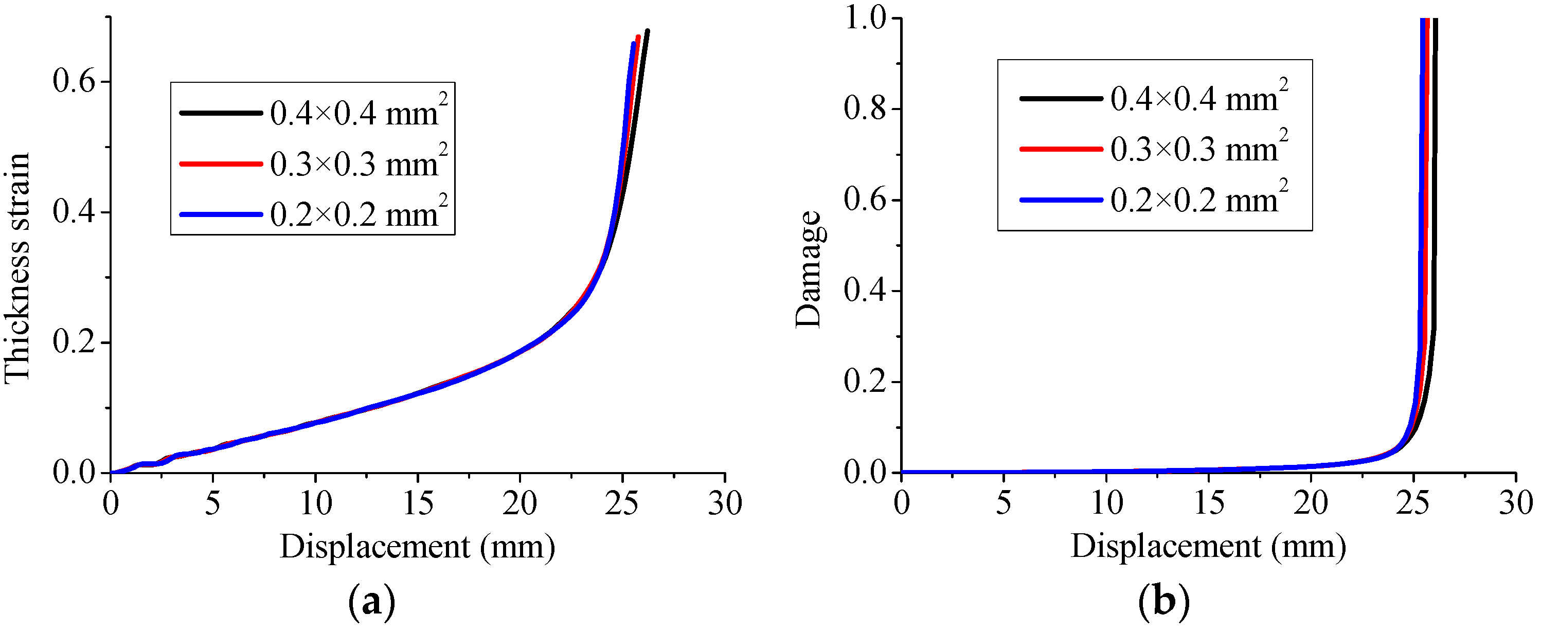
Figure 10.
Effect of the in-plane mesh refinement on the evolution of (a) thickness strain and (b) damage, during the Erichsen deep drawing test for the specimen with 12 mm width.
Figure 10.
Effect of the in-plane mesh refinement on the evolution of (a) thickness strain and (b) damage, during the Erichsen deep drawing test for the specimen with 12 mm width.

Figure 11.
Illustration of the prediction of the occurrence of necking when the thickness strain evolution is taken as indicator.
Figure 11.
Illustration of the prediction of the occurrence of necking when the thickness strain evolution is taken as indicator.
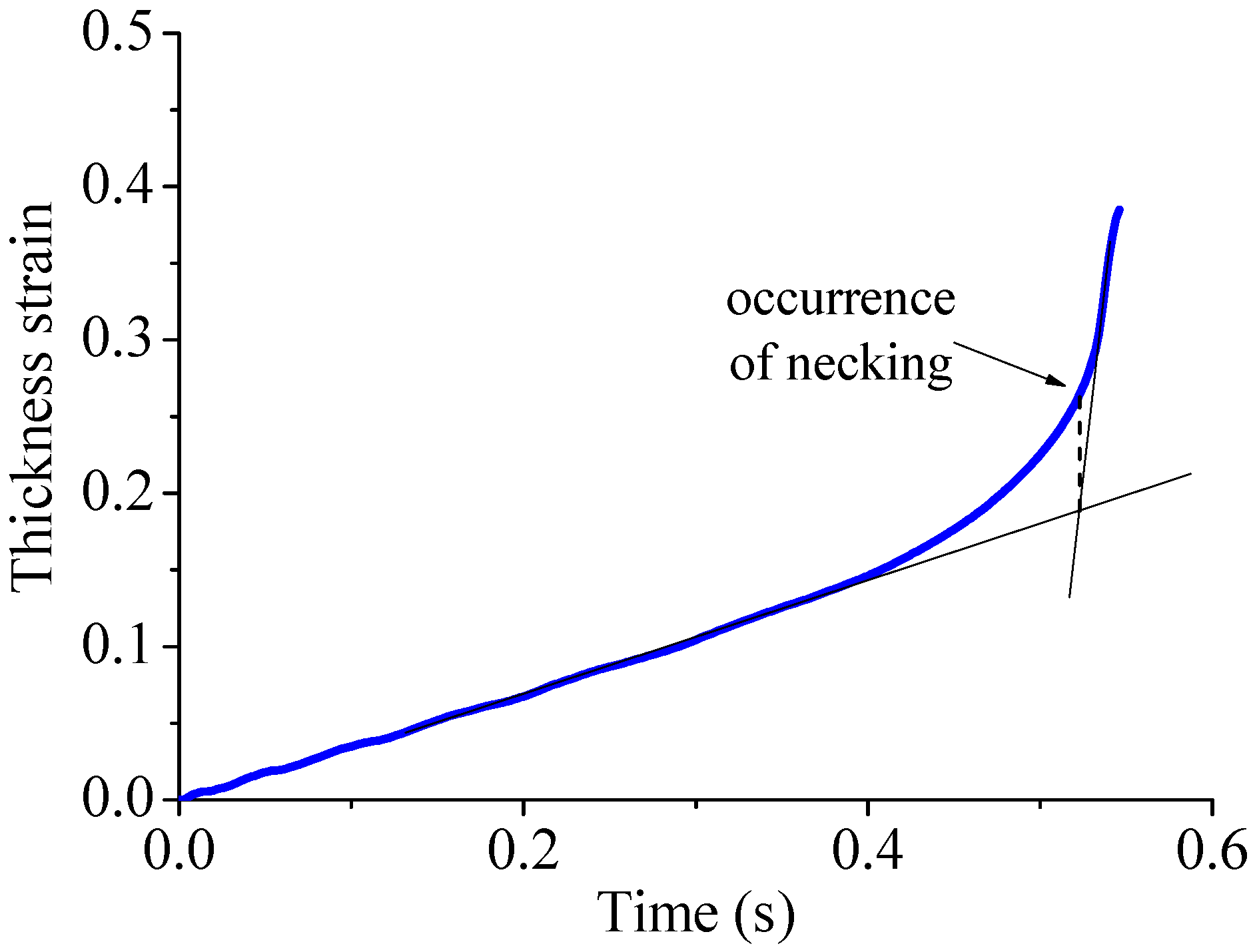
Figure 12.
Illustration of the prediction of the occurrence of necking when the second time derivative of thickness strain is taken as indicator.
Figure 12.
Illustration of the prediction of the occurrence of necking when the second time derivative of thickness strain is taken as indicator.
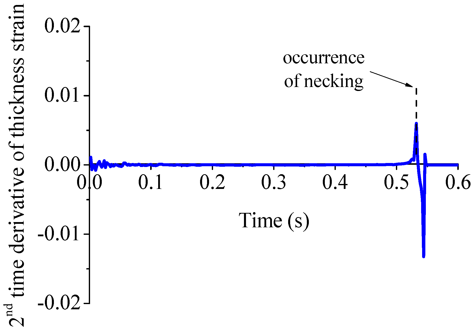
Figure 13.
Illustration of the prediction of the occurrence of necking when the critical damage threshold is taken as indicator.
Figure 13.
Illustration of the prediction of the occurrence of necking when the critical damage threshold is taken as indicator.
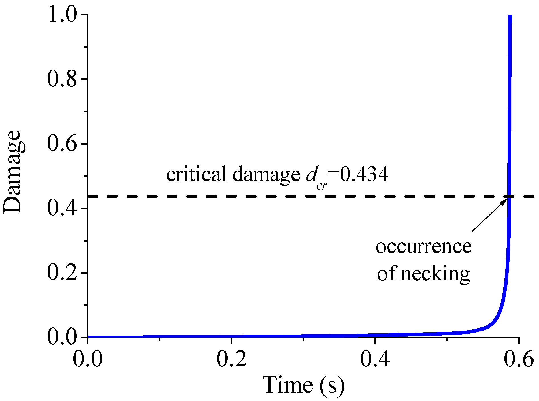
Figure 14.
Numerical load–displacement curves for (a) the simple sheet stretching test and (b) the Erichsen deep drawing test with the various specimen widths.
Figure 14.
Numerical load–displacement curves for (a) the simple sheet stretching test and (b) the Erichsen deep drawing test with the various specimen widths.
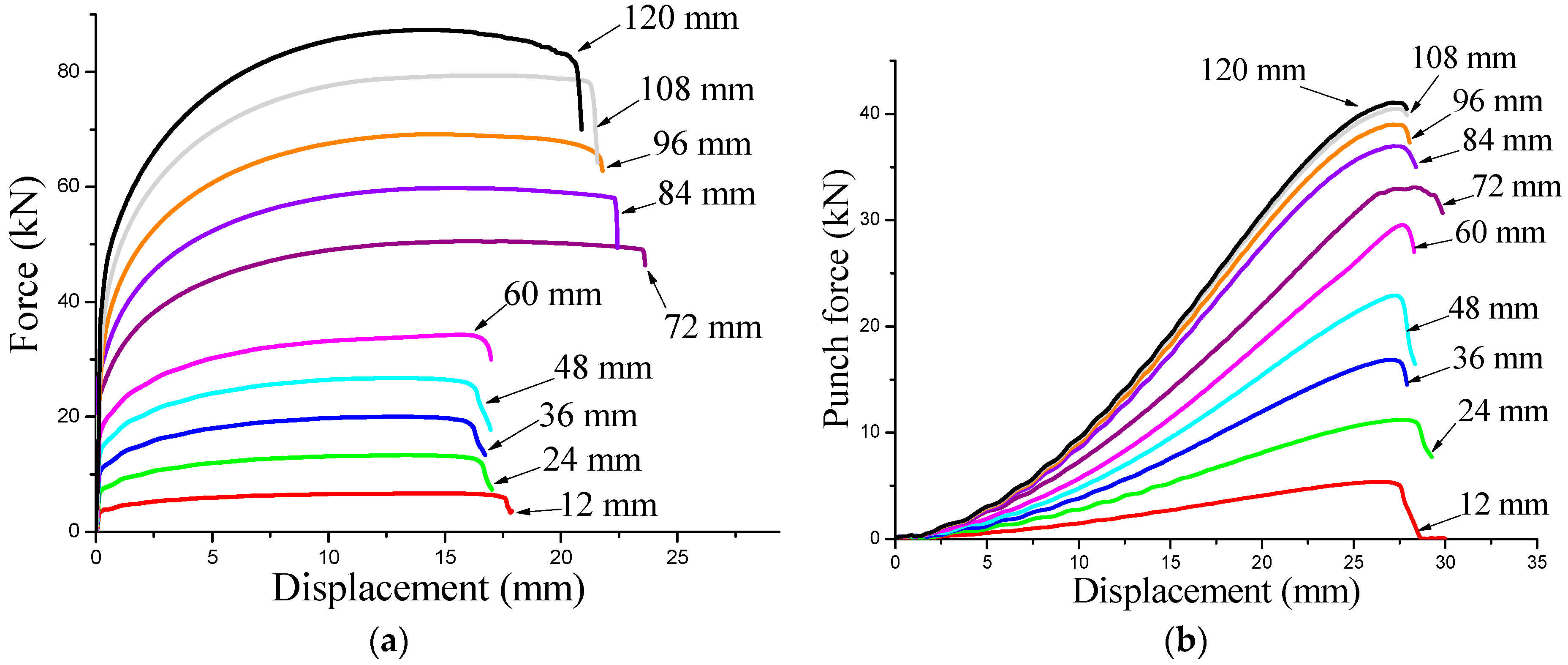
Figure 15.
Distribution of the damage variable, at different stages of loading, as obtained by FE simulation of the simple sheet stretching test with the specimen having a width of 12 mm.
Figure 15.
Distribution of the damage variable, at different stages of loading, as obtained by FE simulation of the simple sheet stretching test with the specimen having a width of 12 mm.


Figure 16.
Distribution of the damage variable, at different stages of loading, as obtained by FE simulation of the Erichsen deep drawing test with the specimen having a width of 24 mm.
Figure 16.
Distribution of the damage variable, at different stages of loading, as obtained by FE simulation of the Erichsen deep drawing test with the specimen having a width of 24 mm.

Figure 17.
Numerical strain paths predicted by FE simulation of (a) the simple sheet stretching test and (b) the Erichsen deep drawing test with the various specimen widths.
Figure 17.
Numerical strain paths predicted by FE simulation of (a) the simple sheet stretching test and (b) the Erichsen deep drawing test with the various specimen widths.
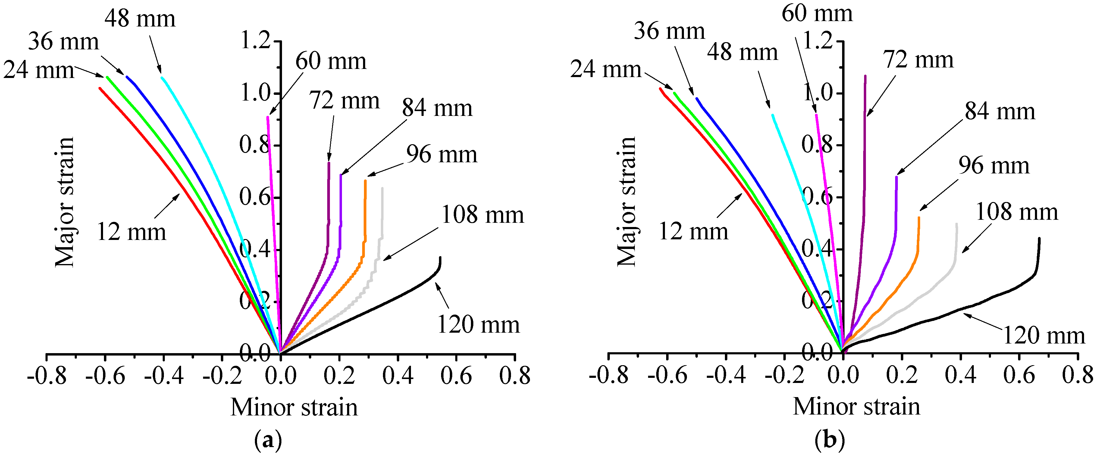
Figure 18.
Forming limit diagram predictions based on the analyses of (a) thickness strain evolution; (b) second time derivative of thickness strain; and (c) critical damage threshold.
Figure 18.
Forming limit diagram predictions based on the analyses of (a) thickness strain evolution; (b) second time derivative of thickness strain; and (c) critical damage threshold.


Table 1.
Elastic–plastic properties for the studied materials.
| Material | E (MPa) | ν | σ0 (MPa) | K (MPa) | n |
|---|---|---|---|---|---|
| Steel | 0.3 | 200 | 0.3–0.6–1.0 |
Table 2.
Lemaitre damage parameters for the studied materials.
| Material | β | S (MPa) | s | Yei (MPa) |
|---|---|---|---|---|
| Steel | 1 | 0.5 | 1 | 0 |
Table 3.
Elastic–plastic properties for the St14 steel.
| Material | E (MPa) | ν | σ0 (MPa) | K (MPa) | n |
|---|---|---|---|---|---|
| St14 | 0.3 | 130 | 585 | 0.44 |
Table 4.
Identified damage parameters for the St14 steel.
| Material | β | S (MPa) | s | Yei (MPa) |
|---|---|---|---|---|
| Steel | 4.251 | 2.648 | 1.831 | 0.001 |
© 2017 by the authors. Licensee MDPI, Basel, Switzerland. This article is an open access article distributed under the terms and conditions of the Creative Commons Attribution (CC BY) license (http://creativecommons.org/licenses/by/4.0/).
Share and Cite
MDPI and ACS Style
Chalal, H.; Abed-Meraim, F. Numerical Predictions of the Occurrence of Necking in Deep Drawing Processes. Metals 2017, 7, 455. https://doi.org/10.3390/met7110455
AMA Style
Chalal H, Abed-Meraim F. Numerical Predictions of the Occurrence of Necking in Deep Drawing Processes. Metals. 2017; 7(11):455. https://doi.org/10.3390/met7110455
Chicago/Turabian StyleChalal, Hocine, and Farid Abed-Meraim. 2017. "Numerical Predictions of the Occurrence of Necking in Deep Drawing Processes" Metals 7, no. 11: 455. https://doi.org/10.3390/met7110455
Note that from the first issue of 2016, this journal uses article numbers instead of page numbers. See further details here.