Detection of Capillary-Mediated Energy Fields on a Grain Boundary Groove: Solid–Liquid Interface Perturbations


1
Florida Institute of Technology, College of Engineering, 150 W. University Blvd, Melbourne, FL 32955, USA
2
School for Engineering of Matter, Transport and Energy, Arizona State University, 551 E. Tyler Mall, Tempe, AZ 85287, USA
*
Author to whom correspondence should be addressed.
Metals 2017, 7(12), 547; https://doi.org/10.3390/met7120547
Submission received: 29 September 2017
/
Revised: 28 November 2017
/
Accepted: 29 November 2017
/
Published: 6 December 2017
(This article belongs to the Special Issue Recent Advances in Study of Solid-Liquid Interfaces and Solidification of Metals)
Abstract
:Grain boundary grooves are common features on polycrystalline solid–liquid interfaces. Their local microstructure can be closely approximated as a “variational” groove, the theoretical profile for which is analyzed here for its Gibbs–Thomson thermo-potential distribution. The distribution of thermo-potentials for a variational groove exhibits gradients tangential to the solid–liquid interface. Energy fluxes stimulated by capillary-mediated tangential gradients are divergent and thus capable of redistributing energy on real or simulated grain boundary grooves. Moreover, the importance of such capillary-mediated energy fields on interfaces is their influence on stability and pattern formation dynamics. The capillary-mediated field expected to be present on a stationary grain boundary groove is verified quantitatively using the multiphase-field approach. Simulation and post-processing measurements fully corroborate the presence and intensity distribution of interfacial cooling, proving that thermodynamically-consistent numerical models already support, without any modification, capillary perturbation fields, the existence of which is currently overlooked in formulations of sharp interface dynamic models.
Keywords:
interfaces; grain boundary grooves; capillarity; pattern formation; phase field measurementsPACS:
81.30.-t; 81.40.-z; 64.70.-K1. Introduction
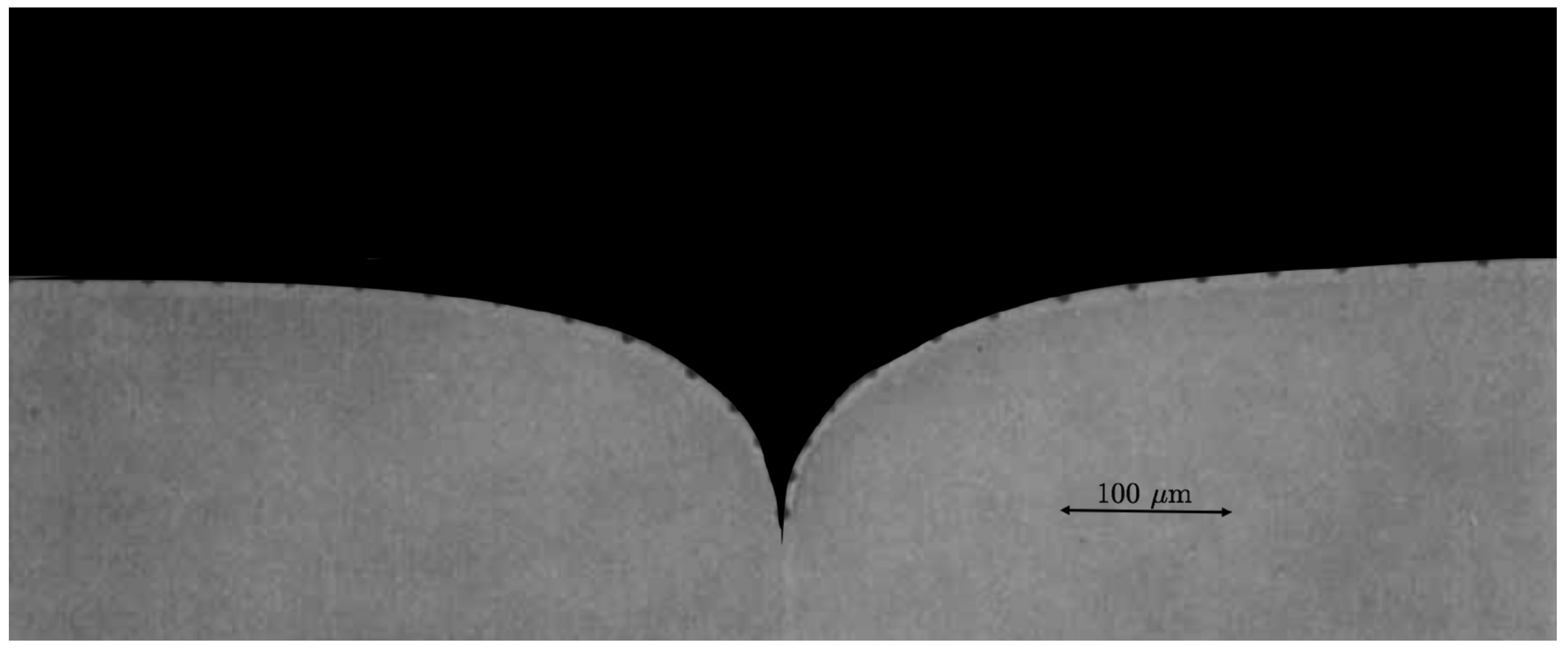
The purpose of this study is to determine by simulation and measurement whether or not interfacial gradients of the Gibbs–Thomson potential distributed along grain boundary grooves also stimulate an energy field along a groove’s solid–liquid interface. Figure 1 shows an example of a grain boundary groove on a stationary solid–liquid interface. The presence of capillary-mediated energy fields was recently postulated [1] to exist on virtually all curved solid–liquid interfaces—both moving and stationary—and provide cooling and heating sources that stimulate complex pattern formation.
A stationary grain boundary groove provides a naturally stable solid–liquid microstructure on which a critical test of the theory predicting the presence of such fields can be performed. Steady-state grain boundary grooves passively communicate heat from their constraining thermal gradient through the surrounding liquid and solid phases, as their stationary interfaces neither produce nor absorb latent heat of transformation, nor are they subject to shape changes or morphological instability. Quite surprisingly, however, the curved configuration of static, solid–liquid grain boundary grooves suggests on the basis of prior analysis [1] that there should be capillary-mediated interface energy fields present, which remain persistently active, despite the groove’s stationarity and the apparent “inertness” of its microstructure.
2. Variational Grain Boundary Grooves
The mathematical shape of a variational grain boundary groove was originally determined by Bolling and Tiller [7]. These investigators found the steady-state theoretical solid–liquid profile in 2D that minimized the total free energy of its microstructure, when constrained by a uniform thermal gradient parallel to the grain boundary. The mathematical term “variational” implies here an analytic groove profile that is a solution to the Euler–Lagrange equation. The Euler–Lagrange equation(s) of variational calculus [8] define the existence of extrema to various classes of functionals, much in the manner of how differential calculus determines both minima or maxima for ordinary functions. Bolling and Tiller’s variational groove profiles provide unique configurations of pure solid and liquid phases, with equal thermal conductivity, arranged so as to minimize their isotropic stored interfacial free energy.
We choose for the present analysis of interfacial energy fields the grain boundary groove shape plotted isometrically in Figure 2. This 2D grain boundary groove has the Bolling–Tiller variational profile, with its intersecting grain boundary oriented parallel to the thermal gradient. The solid–liquid interface and the grain boundary (GB) join, to form at equilibrium, a triple junction located at . Stationary grain boundary grooves exist under conditions of constrained equilibria provided by uniform 1D thermal gradients that produce steady heat flow. The equilibrium dihedral angle of this triple junction, at which the three interfacial tensions balance, is chosen to be , a choice made to enhance phase-field measurements with sharp-interface field theory.
Importantly, this stationary solid–liquid configuration is considered a thermodynamically “open”, steady-state system, insofar as heat is conducted steadily downward through the gradient from hotter liquid through the solid–liquid interface, and into the cooler solid. Solid and liquid phases are assumed to possess identical thermal conductivities, so that the thermal field itself consists of horizontal isotherms and vertical lines of heat flow. The system’s melting point isotherm, , is co-located with the horizontal -axis, or, equivalently, the x-direction.
2.1. Characteristic Size of Grain Boundary Grooves
Dimensionless Cartesian coordinates, , are used in Figure 2 to describe this variational groove’s profile and to formulate its geometric properties. These dimensionless coordinates are and , where x and y represent the groove’s physical coordinates, and is a thermo-capillary length that scales all physical dimensions of the grain boundary groove into numbers. The sizes of grain boundary grooves in most metals and alloys vary between about 1–100 microns, depending on both the material and the magnitude of the thermal gradient constraining the groove. The appropriate scaling length chosen to non-dimensionalize variational grain boundary grooves is defined by their Euler–Lagrange differential equation as,
The material parameters appearing in Equation (1) are: [J/m], the solid–liquid interfacial energy density (assumed isotropic); [m/mol], the molar volume of both phases; and [J/mol·K], the solid–liquid system’s molar entropy of transformation. G [K/m], the system parameter for a grain boundary groove, is the magnitude of the uniform applied thermal gradient that constrains the groove, and controls its size and distribution of interfacial curvature.
2.2. Microstructure Free Energy
The configurational free energy of a variational grain boundary groove consists, in part, of the energies stored along its curved solid–liquid interface and grain boundary. The groove’s solid–liquid interface, which is curved by the “pull” of its grain boundary, increases its total arc length and energy, whereas the grain boundary itself shortens upon equilibration and reduces some of its energy. Undercooled melt contained within the profile’s cusp also contributes excess volume free energy. Specifically, this free energy is proportional to the volumetric entropy change upon freezing of the melt within the groove cusp times its average undercooling. The cusp’s most undercooled point occurs at its triple junction, , across which an angular gap, or “jump”, occurs in the orientation of the normal vector, , along the solid–liquid interface. See again Figure 2. The angular gap defines the groove’s dihedral angle, , which, as mentioned, is chosen to be zero for the current study. Specifically, the choice of zero dihedral angle advantageously provides the deepest possible grain boundary groove cusp, the capillary fields for which prove to have easily identified characteristics, as discussed in detail later in Section 3. Variational groove shapes, moreover, provide unique phase configurations in 2D that minimize their energy per unit distance into the third dimension [J/m], or, equivalently, their total energy [J] for a groove of unit thickness.
The total free energy contained in a variational grain boundary groove is expressed by a functional, , in the plane, which depends explicitly on the groove’s profile coordinates, , and its first derivative . This functional can be “extremized” by applying a standard form of the Euler–Lagrange equation of variational calculus to find the groove profile with the absolute minimum total free energy [8]. The energy functional for the microstructure of a grain boundary groove consists of three contributions as mentioned above: (1) energy added from the extended length of the curved solid–liquid interface; (2) energy reduced from the shortened length of its grain boundary; and (3) free energy added by the undercooled melt within the groove cusp, relative to its stable solid at the same temperature and pressure. The energy functional for a grain boundary groove is formulated as the sum over these three energies (per unit distance into the third dimension), namely,
where the functional’s first term is the total free energy stored in the solid–liquid interface; the second term is the reduction in free energy caused by the shortening of the grain boundary; and the third term is the free energy within the undercooled melt relative to its stable solid.
This energy functional may be reduced to dimensionless form by dividing both sides of Equation (2) by , and recognizing that Young’s force balance for a grain boundary groove with zero dihedral angle holds at the triple junction, , where the grain boundary’s downward pull equals the upward tensions exerted from the two solid–liquid interfaces. Thus, , and if , this balance shows that the ratio . In addition, after the functional’s third term is divided by the resulting lumped parameters may be defined via Equation (1) as the reciprocal thermo-capillary area, [m].
As and , the dimensionless energy functional, , for a grain boundary groove with the profile shown in Figure 2, may be recast in terms of the groove’s dimensionless coordinates as,
2.3. Variational Grooves
Variational grooves are a class of mathematical objects that prove extremely useful for the purposes of thermodynamic field analysis. Their analytic forms, given in Equation (4) for a variational groove with zero dihedral angle, allow accurate estimates to be made of the distribution of their Gibbs–Thomson equilibrium interface thermo-potential, as well as any related (capillary-mediated) vector, or scalar, energy fields that evolve from the presence of that potential. Such fields, we shall show, are extant on thermodynamically equilibrated (real or simulated) grain boundary grooves with the same shape.
Bolling and Tiller [7] found the groove profile that extremizes the energy functional (Equation (2)). The profile shown in Figure 2 is the Bolling–Tiller configuration that minimizes the functional (Equation (3)) and satisfies two additional geometric boundary conditions: (1) the slope of the profile at the triple junction is , corresponding to the dihedral angle ; and (2) the profile becomes flat (zero curvature) far from the groove’s triple junction, where and .
The entire profile in 2D of a variational grain boundary groove with zero dihedral angle, , is described by the dimensionless functions,
The leading plus sign in Equation (4) denotes the variational groove’s right-side profile , and the minus sign denotes its mirror image, left-side profile . See again Figure 2. The pure material’s melting point isotherm, , is coincident with the -axis, with all isotherms above and below parallel to the -axis.
2.4. Equilibrated and Variational Grain Boundary Grooves
Use of the adjective “equilibrated”—in contrast with “variational”—implies a physical, or simulated, grain boundary groove on which full thermodynamic reality is achieved. Full thermodynamic reality connotes an interface supporting every allowed scalar and vector capillary-mediated field. Energy fields consistent with the Gibbs–Thomson interface thermo-potential, its vector gradient and flux fields, and the scalar divergences of those vector fields, are all present on equilibrated grain boundary grooves when local thermodynamic equilibrium is achieved under a constraining applied thermal gradient. The photomicrograph in Figure 1 shows an example of such an equilibrated stationary grain boundary groove. Now, determining whether or not these postulated capillary-mediated energy fields are present on an equilibrated grain boundary groove remains the central quest of this study.
Variational grooves, in contrast with either real (or simulated) equilibrated grooves, do not include or generate any additional interfacial energy fields to those specified in its energy functional (Equation (2)). The explanation for this limitation is that although solid–liquid capillarity is responsible for the development of a specific Gibbs–Thomson potential distribution along the curved solid–liquid interface of a variational grain boundary groove, its presence as an interface field is admitted solely as a scalar thermodynamic potential. This scalar field serves, in the case of variational grooves, to ensure that a match exists between the local thermodynamic activities of the groove’s curved solid phase and its undercooled melt. Beyond its “activity-matching” function, the Gibbs–Thomson potential does nothing further for variational grain boundary grooves, such as eliciting interfacial gradients and fluxes of either energy or matter.
Despite the ostensible presence of an interfacial gradient field associated with the Gibbs–Thomson potential, its vector flux and energy fields are simply excluded. Inclusion in the standard variational formulation of any additional capillary-mediated fields—beyond just the Gibbs–Thomson’s interface scalar potential—would introduce nonlinear terms into the groove’s energy functional, Equation (2), and preclude, or at least complicate, finding analytic solutions for the variational extremum from the variational calculus formulation.
We show next that the associated vector gradient field of the Gibbs–Thomson potential along an equilibrated grain boundary groove does provide vector energy fields, i.e., tangential thermal fluxes, the divergence of which support additional scalar energy rates that influence the interface’s local energy budget. Note, moreover, that scalar energy fields of similar origin are present on moving solid–liquid interfaces that act as “perturbations”, which stimulate pattern formation during solidification.
3. Thermo-Potential on Variational Grooves
Curvature of a solid–liquid interface, in the presence of capillarity, induces a small shift of the solid–liquid equilibrium temperature, , relative to the material’s normal melting point, [K], measured at a flat interface. The direction of the equilibrium shift depends on the sign of the curvature: geometrically convex interfaces have slightly lower equilibrium temperatures than do flat or concave interfaces. The amount of induced temperature shift is specified by the well-known Gibbs–Thomson condition [9]:
where [m] is the in-plane local curvature along a 2D solid–liquid interface.
One may remove temperature [K] from both sides of Equation (5) and create a thermo-potential, by dividing through by an appropriate temperature interval, chosen here for variational grain boundary grooves as [K]. This temperature interval equals the magnitude, G, of the uniform thermal gradient in which a grain boundary groove is equilibrated, multiplied by a distance along that gradient sampled by the grain boundary groove—a distance which is proportional to its cusp depth. That distance, , is defined in Equation (1) from the groove profile’s Euler–Lagrange differential equation [8]. These steps yield the dimensionless thermo-capillary potential, , appropriate to the solid–liquid interface of a grain boundary groove,
Next, a dimensionless curvature may be defined for a grain boundary groove’s solid–liquid interface as , by multiplying the local interface curvature by twice the groove’s characteristic length, . Thus, the geometric curvature [m] in Equation (6) may be replaced by by inserting a compensating factor of into the denominator of the lumped material and system constants. These steps yield a scaled form of the thermo-potential for a variational grain boundary groove as
Finally, the five constants grouped on the right-hand side of Equation (7) are set equal to unity by virtue of Equation (1), so the dimensionless Gibbs–Thomson interface potential, , along a variational grain boundary groove is equal to (minus) its dimensionless curvature:
3.1. Curvature of Variational Profiles
The dimensionless interface curvature, , (taken here as a positive number) may be calculated for the profile of a variational grain boundary groove by applying the standard Cartesian formula for curvature to its profile, Equation (4). In 2D, the in-plane curvature for the selected groove profile, , is calculated as
The first and second derivatives of the right- and left-side variational groove profiles have opposite signs, and are respectively:
Substituting these expressions for the derivatives required in Equation (9), and simplifying the result, establishes an important linear relationship between local interface curvature and the cusp depth, , for a variational grain boundary groove,
Combining Equations (8) and (10) shows that the dimensionless Gibbs–Thomson thermo-potential and (minus) the groove’s dimensionless curvature are the same numbers, which equal four times the groove’s -coordinate,
Equation (11) interrelates thermodynamic potential, curvature, and dimensionless groove depth, and, as already described in Section 2.4, exposes several self-consistent features regarding the configuration of a variational groove and its thermodynamic behavior, all of which may now be exploited using field-theory.
3.2. Gradient of the Gibbs–Thomson Thermo-Potential
Tangential gradients of a thermodynamic potential, such as the Gibbs–Thomson equilibrium temperature, provide the necessary condition for the appearance of a capillary-mediated flux of thermal energy directed opposite to its gradient vector. The condition for sufficiency, needed for the actual on-set of such an interfacial flux, is a non-zero transport number, or conductance. The well-studied phenomena of species diffusion along solid–solid interfaces and over free surfaces—both analogous transport phenomena to what is under consideration—show that at temperatures even well below the melting point of a material, interfacial conductances are, in fact, always non-zero [10]. One therefore always expects some finite transport to occur along solid–liquid interfaces when impressed by gradients.
Surface diffusion processes, however, have gained considerable importance in diverse applications such as catalysis, sintering, and grain growth. Superficial heat conduction, the topic being discussed here, has received by contrast scant attention, as interfacial thermal conduction is a 2nd-order transport phenomenon relative to ordinary volumetric (bulk) heat transfer. Nevertheless, as a perturbative phenomenon, even small, capillary-mediated, thermal effects must be considered in the interfacial energy budget of a solid–liquid system.
Perhaps the transport phenomenon most closely associated with capillary-mediated interface heat conduction, but already studied in impressive detail, is Bénard–Marangoni hydrodynamic flow. Bénard–Marangoni flow is induced on fluid–vapor interfaces by superficial tangential thermal gradients [11]. These flows, however, result from direct fluid-mechanical responses to thermal gradients that imbalance surface tension forces, whereas interface thermal conduction fields analyzed in this study result indirectly from the higher-order divergence of the capillary-mediated interfacial heat flux, and not, per se, from the direct action of the potential gradient.
The 2D gradient field of the Gibbs–Thomson potential along a variational grain boundary groove is determined by calculating the arc-length derivative, , of the potential, , from Equation (11). This directional derivative is taken with respect to dimensionless arc length, , tangentially along the groove’s solid–liquid profile. Interfacial arc length, s, is scaled similarly by dividing it by twice the thermo-capillary length, , which yields the following operational sequence for obtaining the tangential gradient in 2D of the Gibbs–Thomson thermo-potential,
Here, the arc length derivatives of the variational groove’s independent variables, namely, , are found to be positive along the groove’s left profile, and negative along its right profile, so one finds that
3.3. Capillary-Mediated Fluxes
Fourier’s law of heat conduction [12] relates heat fluxes to their associated thermal gradient and heat conductance. In 2D, a tangential (interfacial) flux of energy bears physical units of [watts/m], and its corresponding interfacial thermal conductivity, , assumes the appropriate physical units of [watts/K].
Tangential energy fluxes, as do surface diffusion (species) fluxes, are directed antiparallel to their arc-length gradients, , Equation (14). The resulting capillary-mediated flux along the interface of an equilibrated grain boundary groove (based on the profile of its corresponding variational profile) is described by the same quadratic form as that of (minus) the dimensionless Gibbs–Thomson gradient, cf., Equation (14),
Plots of the vector magnitude of Equation (15), shown in Figure 3, indicate that capillary-mediated thermal fluxes fade to zero along the flatter portions of the grain boundary groove’s solid–liquid interface where . Their magnitudes also increase steadily toward a maximum at the groove’s triple junction, . The tangential directions of the right- and left-interface thermal fluxes counter-rotate as they approach each other, and finally become parallel to their common -axis where they meet at the triple junction of a grain boundary groove with zero dihedral angle. The resultant left and right thermal flux combine and enter the grain boundary as a steady current of capillary-mediated energy. This energy flow, we shall show, continues indefinitely.
Capillary-mediated fluxes remain tangential to the solid–liquid interface, and, consequently, do not directly affect the interfacial energy budget, as do flux components that are directed normal to the interface. That fact seems to comport with conventional wisdom, expressed, for example, by the Stefan energy balance, which considers only energy flux components that are directed normal to the solid–liquid interface. Such normal fluxes arise from heat conduction, latent heat evolution, and thermal radiation [13]. However, we show next that energy conservation along a solid–liquid interface must be satisfied “omnimetrically”. That is, energy accumulation at every point on an interface must balance to zero over all continuum length scales. As Stefan’s energy balance lacks capillarity, it consequently fails to satisfy this essential physical requirement on real solid–liquid interfaces: Namely, energy conservation at all continuum scales.
3.4. Capillary Flux Divergence
Tangential heat fluxes travel along the interface in a direction that is orthogonal to the normal flux components included in Stefan’s energy balance. Despite their apparent “pass through” nature, capillary-mediated tangential heat fluxes do, in fact, affect an interface’s energy balance. Specifically, tangential fluxes act indirectly, by releasing and/or removing energy along the interface via their vector divergences. Field theory shows, moreover, that flux divergences at a point on an interface create equivalent sinks, or sources, that remove, or add, energy at that point. Capillary flux divergences currently under discussion are termed “bias fields”, so named because they affect an interface’s energy budget, and bias its local velocity slightly above, or below, the average rate established by Stefan’s (capillary-free) energy balance. Capillary-mediated flux divergences tend to become significant where the interfacial curvature and its spatial derivatives become large. Formulas for the interface bias field in isotropic systems involve nonlinear combinations of the curvature and its first two spatial derivatives [1]. These nonlinear dependences involve subtle 4th-order features of the interface shape. Consequently, the strength of capillary flux divergences depend sensitively on the spatial distribution of curvature along an interface. which occur typically on evolving solid–liquid interfaces over mesoscopic scales, i.e., from about 10 nm up to several mm.
We note that quasi-static thermal fields within bulk solid and liquid phases obey Laplace’s equation that guarantees their volume heat fluxes are non-divergent. Superficial capillary-mediated fluxes traveling tangentially on the solid–liquid interface of an equilibrated grain boundary groove are, by contrast, divergent, and are described instead by Poisson’s equation [1], namely,
where the right-hand side of Equation (16), , equals the Poisson source strength, and defines the capillary-mediated bias field function. The superficial, or surface Laplacian operator in 2D, , appearing in Equation (16), may be obtained by twice applying the chain rule for arc length differentiation. The following nested set of elementary operations yields as the 2D surface Laplacian of the Gibbs–Thomson potential,
Inserting Equation (11) for the groove’s Gibbs–Thomson thermo-potential into Equation (17), and twice applying the groove’s arc-length derivative (Equation (13)) show that the surface Laplacian of the Gibbs–Thomson thermo-potential for a variational grain boundary groove is a (negative) cubic function over the -range of the groove, the Poisson equation for which is
Thus, potential theory shows, perhaps surprisingly, that capillary-induced heat removal—i.e., interfacial cooling—is present on stationary grain boundary grooves from the divergent vector gradient and flux of the groove’s scalar thermo-potential. The intensity of this persistent heat removal, termed the bias field, is plotted as a function of groove depth in Figure 4. As shown, an equilibrated grain boundary groove continually loses some heat everywhere along its solid–liquid interface, but mainly within its groove cusp.
3.5. Cooling Distribution
The distribution of cooling rates along the -axis may be found by cross-plotting the cooling intensity, (Equation (18)) against the variational profile, . The left and right cooling distributions, , are plotted in Figure 5 for an equilibrated grain boundary groove with zero dihedral angle.
This distribution shows that the entire solid–liquid interface is subject to some rate of capillary-driven heat removal, particularly in the region surrounding the groove’s triple junction, , where the cusp steepens significantly, . One also sees that cooling is predicted to be strongest at the twin valleys of this distribution. The exact -values at which cooling rate maxima occur are , see also Figure 5. Interfacial cooling rates then rapidly decay as either the triple junction is approached and , or as the interface flattens and .
4. Detecting Interfacial Energy Fields
4.1. Proportionality of Potential and Heat Rate
If capillary-mediated cooling actually exists along an equilibrated grain boundary groove, then its presence should affect the linear distribution of thermo-potential predicted for its counterpart variational grain boundary groove that, as explained in Section 2.4, lacks a capillary-mediated bias field. Detecting small nonlinear departures of a nearly linear potential distribution remains the essential challenge to making phase-field measurements that uncover the existence of an active capillary field on a solid–liquid interface and determine its distribution of energy removal rates over the interface.
Specifically, cooling along a grain boundary groove’s solid–liquid interface adds a small nonlinear component to the interface potential. This nonlinear addition to the interface potential is proportional to the rate of thermal energy added to each point by the capillary bias field: i.e., if the interface is cooled at a point, its total thermo-potential at that location is lowered and made more negative in proportion to the cooling rate. If the interface instead were heated, then its potential would rise by an amount proportional to that heating rate. Finally, if the bias field did not exist, the interface potential along a grain boundary groove would be unaffected, and its distribution would remain linear with its depth coordinate.
The proportional linkage between thermal energy, Q, and the change in temperature, or thermo-potential, in both closed and open systems is based on the relationship between conjugate thermodynamic variables: viz., the entropy, S, and temperature T, the product of which is energy. Specifically, if the enthalpy, —a Legendre transform of the energy that also equals the “heat content” at constant pressure, P—increases or decreases, one finds that . Then, assuming that no work is performed, the derivative of enthalpy with respect to temperature at constant pressure is equal to—indeed defines—the phase’s specific heat , where . This “calorimetric” relationship demonstrates the proportionality between small changes in temperature, or thermo-potential, and heat supplied or removed, namely,
See also reference [14], Equation (4.42), and its formal discussion on pp. 52–55, that prove the proportional relationships of heat content, enthalpy, and temperature changes occurring in pure substances at constant pressure.
The proportionality (Equation (19)) between the heat release or absorption and the induced temperature change also provides the fundamental basis for thermal analysis instruments such as adiabatic drop calorimeters and scanning differential thermal analyzers (DTA). Moreover, for small temperature intervals, as encountered here with capillary-mediated energy fields on solid–liquid interfaces, changes in interfacial heat rates and the local interface temperature shift remain precisely proportionate.
Lastly, the general relationship between interfacial energy rate and steady-state local potential also has a firm mathematical foundation based on standard scalar potential theory, insofar as the strengths of point sinks, or point sources, released steadily along boundaries may be represented mathematically as line integrals of their Green’s function distributions [15]. Some specific examples of this expected proportionate response for both instantaneous and continuous diffusion sources, as represented by their Green’s functions distributed along planar and circular boundaries in different spatial settings, are discussed in [16]. Those cited examples demonstrate quite generally that steady-state interfacial source rates of conjugate extensive quantities, such as enthalpy, mass, and strain volume, induce proportionate changes on a boundary’s intensive thermo-potential, species concentration, and stress, respectively.
4.2. Sharp and Diffuse Interfaces
Interface bias fields caused by capillarity were discovered as mathematical entities derived analytically from sharp-interface thermodynamics using classical potential theory [1,17]. By distinction, phase-field models deal with continuously varying phase domains that allow the numerical solution of time-dependent coupled partial differential equations. Phase field models, moreover, simulate thermodynamic behavior of multiphase systems with diffuse, not sharp interfaces—and this point is extremely important—despite the fact that phase field models are not coded with any explicit physics that directly admit or require spontaneous interface energy fields. Phase-field modeling therefore provides completely independent inquiry assessing the presence, or absence—and even the measurement—of capillary-mediated energy fields.
In short, the ability to equilibrate a simulated stationary grain boundary groove with diffuse interfaces, to ‘uncover’ and measure its resident capillary-mediated energy field, presents the opportunity for using a phase-field model to verify interfacial thermodynamic behavior consistent with predictions from sharp interface theory. We proceed in the next section with a brief summary of the entropy-based multiphase-field model that was used here to simulate a grain boundary groove’s microstructure with zero dihedral angle, and then equilibrate it accurately in a uniform 1D thermal gradient. In the interest of brevity, full details are not explained about the measurement of isoline thermo-potentials and their residuals, all of which were calculated from the phase-field data via a post-processing algorithm. The equations and their parameters for computing multiphase-field simulations are now well established and discussed by many sources, and the interested reader can obtain further details of multiphase-field theory and its numerical implementation from the literature. The subject of numerical modeling diffuse heterophase interfaces is indeed now a large one, and we hope that this initial study, exposing the presence of capillary-mediated interface fields by using phase-field modeling of stationary grain boundary grooves, will stimulate interest to pursue its many details and ramifications for solidifying alloys and other more complicated systems of interest.
5. Numerical Model and Results
5.1. Multiphase-Field Model
We employed the following entropy density functional for multiphase-field computations of thermal grain boundary grooving,
This phase-field model ensures consistency with classical irreversible thermodynamics. The bulk entropy density, , depends on the internal energy density, e, where is a vector of phase-field variables that lies in the dimensional plane. N, in general, represents the total number of grains and phases. In the present simulations, we identified 3 phase-fields to represent crystal-1 (), crystal-2 ()—i.e., the two grains separated symmetrically by the grain boundary—and their common pure melt phase (), configured as the grain boundary grooves in Figure 1 and Figure 2. The functions and represent the gradient and obstacle-potential energy density, respectively; is a small length scale parameter related to the thickness of the simulated diffuse interface, and V represents the domain volume [18,19].
The pair of governing equations that account for energy conservation as a function of temperature, T, and the non-conserved phase-field variables, , derive from the functional, Equation (20), as
and
The quantities and are, respectively, variational derivatives of the entropy functional, , with respect to energy, e, and phase variable, . The parameter denotes the mobility governing interface kinetics, whereas the mobility coefficient, , is related to the system’s thermal conductivity, , which is assumed to be equal for both phases. The choice of equal thermal conductivity for both phases, as explained in Section 5.1 and Section 5.2, is needed here to compare phase-field measurements of a solid–liquid interface potential distribution with that for the corresponding variational grain boundary groove, the analytic profile for which (Equation (4)) also depends on the assumption of equal thermal conductivities. Unequal thermal conductivities of the solid and liquid at equilibrium in a thermal gradient produce an active thermal field along the interface that leads to significant shape change from the profile of a field-free (equal conductivity) variational grain boundary groove. The interfacial field and the equilibrium grain boundary groove shape for various thermal conductivity ratios were calculated from field theory, and confirmed experimentally by using an electrical analog [20].
The internal energy density, e, is related to the molar latent heat, , and constant specific heat , by the relationship . The interpolation function satisfies the constraints and .
Evolution of the temperature field over the 2D domain can be derived from Equation (21), the energy equation, given that the variation of the phase energy, e, with respect to its entropy, , defines the thermodynamic temperature, T, of a pure material; thus, . Substitution of the reciprocal temperature into Equation (21) and then carrying out the gradient and divergence operations yields the temporal equation for the thermal field,
Here, is the thermal diffusivity, and is the system’s characteristic adiabatic temperature. Equation (22) and the Legendre transform, , allow the kinetic equation for phase-field order parameters to be written as
where is a Lagrange parameter that maintains a unitary constraint on the sum of all local phase indicators, so that . For the terms ; ; ; and , each denote partial derivatives with respect to and .
The phase-field model parameters described above were non-dimensionalized by selecting a capillary length scale, and a characteristic conduction time, . In carrying out the numerical simulations, we chose dimensionless values for (again, assumed equal in both the crystals and their melt); ; interfacial energy, ; interface mobility, ; and the melting temperature, .
5.2. Fidelity of the Groove Equilibration
An explicit finite-difference discretization scheme was employed for iteratively solving Equations (23) and (24) in a 2D domain of grid size . The thermal diffusivities of both crystalline grains and their melt were chosen to be equal for strict compliance with the equal conductivity assumption critically required in the case of variational groove profiles. The thermal gradient, G, imposed normally on the initial planar crystal/melt interface allowed the temperature to vary linearly from a minimum value of along the bottom edge of the computational domain to a maximum value of along its top.
The following steps were followed to assure that the groove’s evolved dihedral angle corresponded to that predicted via Young’s force equilibrium at the triple junction, and that the simulated groove profile achieved full equilibration:
- We set the ratio of the grain boundary’s energy density equal to twice that of the crystal/melt boundary, so chosen to produce after steady-state equilibration the desired dihedral angle of . (Refer to Section 2.2 and reference [21] for further details on this point.).
- We checked carefully that the required uniform 1D thermal gradient and its linear temperature distribution developed fully along the phase-field Y-grid ordinate scale of the evolved grain boundary groove.
- We measured the dihedral angle at each time-step [22]. After the dihedral angle approached its expected equilibrium value of zero, we continued further equilibration for an additional time-steps. This assured that any further relaxation would not occur on the equilibrated groove profile that could otherwise alter its shape and thermo-potential distribution surrounding the triple-junction region.
As this study will show, phase-field models incorporate within their physics equivalent capillary-mediated perturbation fields for curved, slightly diffuse, stationary solid–liquid interfaces. The same, we believe, may be said for other thermodynamically consistent dynamic interface models. We also found that the number of grid points comprising the diffuse crystal-melt interface were far greater at highly curved regions within the groove cusp, compared to those portions of the interface far from the groove’s triple junction, where the crystal-melt boundary remained relatively flat. The disparity in the number of grid points defining the diffuse interface degraded the accuracy of our potential measurements taken over flatter regions of the solid–liquid interface. To maintain good accuracy everywhere when extracting crystal-melt potentials, , along the interfacial isoline, irrespective of the interface’s local curvature, we employed a numeric phase indicator for with the resolution range of .
5.3. Post-Processing Residuals and Interface Fields
In accordance with the Gibbs–Thomson equilibrium condition, the steady-state potential and curvature distributions along the profile of a variational grain boundary groove, which has zero interfacial thickness, are guaranteed to be perfectly linear in the depth variable . See again Equations (7) and (11). Therefore, if one were to subtract the dimensionless value of the constraining linear thermal potential, , from the variational groove’s interface potential, , one would obtain uninteresting residuals, , because Equation (11) shows that .
Now contrast what happens upon numerically simulating an equilibrated grain boundary groove with a phase-field numerical model, where superficial gradients of the simulated interface potential can appear along the diffuse interface’s isoline, for . Presumably, these gradients induce a divergent tangential flux, similar to that predicted by Equation (18), with a cooling distribution configured like the one plotted in Figure 5. A distribution of interfacial sinks of thermal energy rate, , so created along the isoline , by virtue of which the dimensionless temperature, or thermo-potential distribution, , along that isoline becomes slightly depressed and departs from its linear form. Consequently, the simulated residual of the thermo-potential, , after achieving full equilibration in a uniform applied gradient, G, is calculated as . Equilibrated residuals are then measured point-wise along the isoline . Our estimate for the mean relative error of post-processed residuals is .
The measured residual of the thermo-potential (multiplied by is postulated to equal the interfacial cooling rate at that point, , divided by the ratio, , that best aligned the largest theoretical rate of energy withdrawal rate, , with the largest observed isoline potential residual, . Thus, applying the proportionality found between thermo-potential shift, or residual, and the local interfacial heat rate, one finds that
We posit that an interfacial rate of cooling intensity, , exists at points along the solid–liquid interface where we measure the induced nonlinear residuals in the interface’s isoline potential. The cooling intensities, or negative heating rates, responsible for the observed residuals are therefore,
Perhaps more convincing, one also finds that the cooling rate distribution, , found along the equilibrated phase-field isoline conforms closely with the energy field’s theoretical distribution, , calculated for the simulated groove’s counterpart variational groove from Equation (18), and displayed in Figure 5.
Finally, we note that the proportionality explained in Section 4.1 between simulated potential residuals of equilibrated grain boundary grooves and the theoretical bias field of a variational groove is actually slightly inexact. An imperfection is expected because we have ignored higher-order differences that exist between the analytic variational profile (viz., Equation (4)) and the actual equilibrated shape of the simulated grain boundary groove. The curvatures of real and simulated equilibrated grain boundary grooves must increase slightly at all points relative to those of their variational counterpart profiles to account for the depression of their local thermo-potentials from capillary-induced cooling. These self-interactive nonlinear shape changes are, however, extremely small—estimated to be of only 4th-order—so that the analytic perturbation field of the variational grain boundary groove, which is easily calculated from Equation (18), does closely approximate isoline residuals data obtained by multiphase-field simulation and measurement.
5.4. Interface Potential Residuals
One must allow the simulated grain boundary groove in a uniform 1D thermal gradient to achieve its fully equilibrated steady-state configuration in order to gather, with sufficient precision, residuals of the interface potential. Achieving full equilibration ensures that the simulated groove profile is thermodynamically self-consistent with its interfacial potential, as already discussed in Section 4.2. Cooling fields were exposed and measured during simulation as residuals of the interface’s thermo-potential, per Equations (25) and (26). We measured these residuals in situ along the interface isoline using a post-processing algorithm. Numerical details revealing the presence of interface fields are explained next. Phase-field simulations not only allow precise measurement of a stationary interface’s equilibrated potential distribution, but are also capable of resolving isoline potentials at levels of spatial resolution well beyond those that could be accomplished using any currently available experimental techniques.
The equilibrated groove profile, upon which potential measurements were made, must not, however, be so different from that of its variational counterpart, on which are based the Gibbs–Thomson distribution and its dependent capillary energy fields expressed through Equations (8), (15), and (18). A significant difference between the variational profile and the simulated equilibrated profile would preclude quantitative comparison between simulation results and sharp interface predictions. Such thermal conditioning of a simulated grain boundary groove requires precise thermodynamic equilibration achievable only after lengthy simulation runs requiring several hundred thousand phase-field numerical iterations. Once fully equilibrated, however, the cooling perturbation that developed on a grain boundary groove microstructure remains active and persistent along its simulated interfacial isoline. The cooling field’s intensity and spatial characteristics may be precisely quantified through measurement of nonlinear residuals detected numerically along the simulated profile, or isoline. Precise potential residuals, accurate to within ppm, were measured point-wise by subtracting from the isoline’s slightly nonlinear potential distribution the known linear potential distribution imposed by the 1D uniform gradient specified in the simulation during equilibration. See Equation (25).
Note again, if an active capillary field were not present along a groove’s interfacial isoline, and thus not distorting its otherwise linear potential, then its calculated residual would result in a mean-zero (null) difference. Instead, we observed a smoothly varying distribution of non-zero residuals that, as explained in Section 4.1, are themselves directly proportional to the strength of capillary-induced cooling acting along the solid-liquid interface. Measurement of the resident isoline cooling rate distribution, of course, also allows comparison with the theoretical cooling distribution already predicted independently from the Gibbs–Thomson thermo-potential and displayed in Figure 5 for a variational grain boundary groove with zero dihedral angle.
5.5. Nonlinear Residuals of the Thermo-Potential
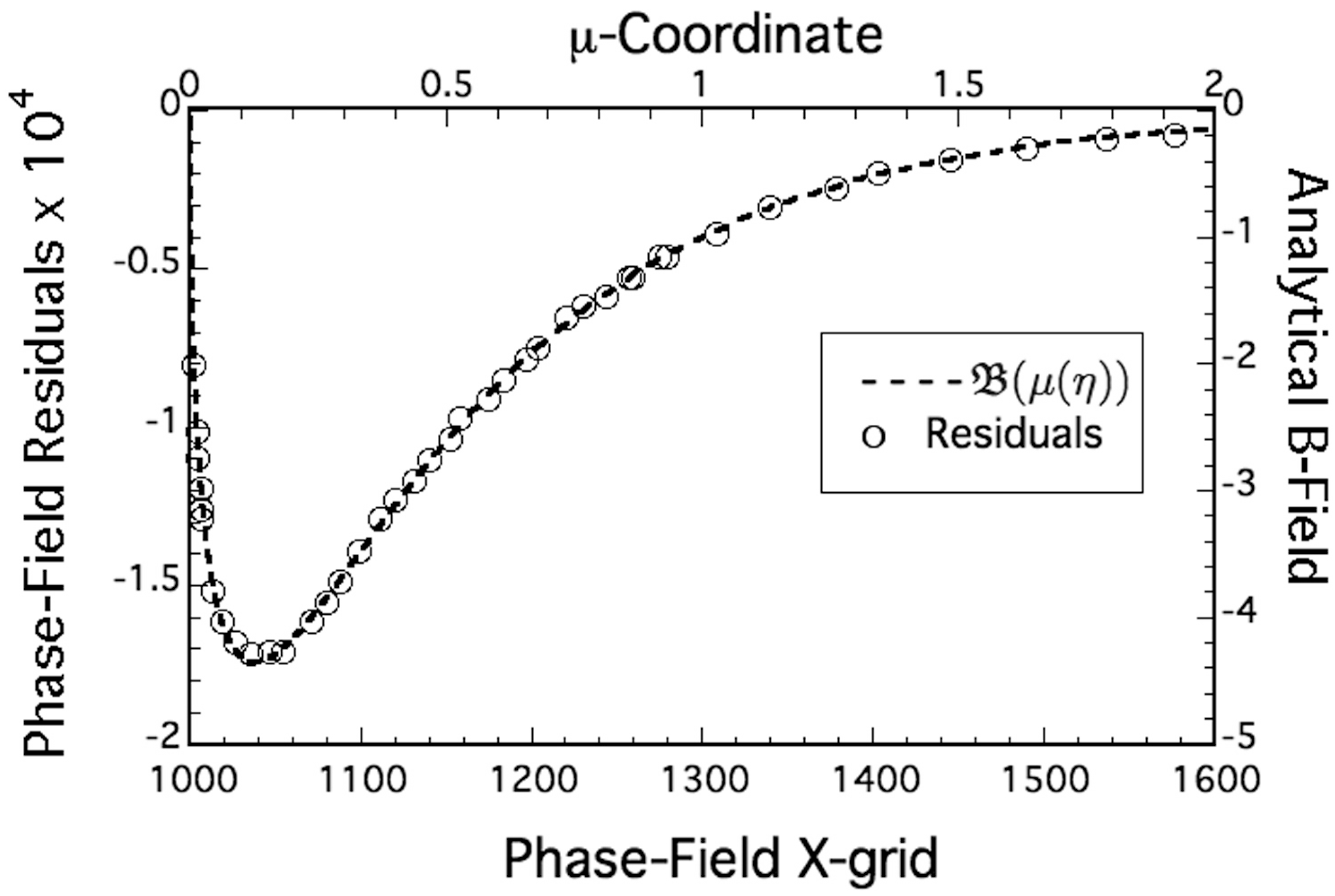
The measured phase-field residual data from simulations and the predicted rate distribution, , are plotted together in Figure 6. The equilibration of the simulated grain boundary groove involves many choices for all the simulation parameters needed to equilibrated a two-phase groove microstructure that is comparable with a variational grain boundary groove with zero dihedral angle. These parametric choices, for example, include selecting the computational domain size, interface thickness, dihedral angle, thermal gradient, thermal conductivity, interfacial and grain boundary energies, etc.
Comparison of simulated interface potentials and their nonlinear residuals to heat removal rates predicted for the theoretical bias-field on a sharp interface requires: (1) selecting an independent computational scale (X-grid) used during simulation that matches the (arbitrary) dimensionless -scale used to plot the cooling distribution in Figure 5 and Figure 6; and (2) finding the amplitude ratio of the maximum measured potential residual to the largest heat removal rate predicted from sharp interface theory. The selection of length scale and amplitude ratio allow all residuals of the simulated thermo-potentials to be compared with the theoretical -field cooling rate without further adjustment.
Attempting absolute comparison between simulated quantities and the bias-field, however desirable as a goal, remains out of reach at present, given our lack of knowledge about interface thermal conductances on solid–liquid interfaces. We therefore chose the ratio (300:1) between the X-grid (minus 1000) simulated abscissa values with those for the arbitrary dimensionless -coordinate scale, and applied a right-to-left ordinate ratio (2.50:1) that matches the maximum phase-field residual ×10 with the predicted value for the maximum dimensionless theoretical cooling rate calculated from Equation (18). These two ratios allow all measured phase-field residuals to track the distinctive shape of the bias-field distribution calculated for a sharp interface grain boundary groove with zero dihedral angle.
Although these data are, to our knowledge, the first such results obtained for any microstructure, they demonstrate that precision simulation data align with sharp interface predictions over the entire profile of a grain boundary groove. The present results also indicate that phase-field modeling simulates thermodynamically realistic microstructures exhibiting interfacial energy fields that are consistent with those predicted from field theory. We plan to pursue additional testing of other microstructures for their presence of deterministic capillary-mediated energy fields that affect diffusion-limited interface patterns.
6. Conclusions
Residuals data measured and plotted in the manner described in Section 5 mimic the distribution of cooling rates for an equilibrated zero dihedral-angle grain boundary groove, and allow comparison with its counterpart variational profile (Equation (4)). Close correspondences of the interfacial energy fields were found for the simulated and variational grain boundary grooves, which accurately portray the predicted “valley” in the interface cooling rate, followed by a rapid fall-off in the cooling intensity toward flatter regions of the solid–liquid interface. Thus, both the overall shape of the cooling distribution, as well as the position and amplitude of the most intense cooling rate within the equilibrated groove cusp are all captured with a single proportionating factor linking simulation and analysis. Moreover, the density and fidelity of residuals data, and the predicted -field for the corresponding variational groove, show that persistent capillary-mediated fields exist on stationary curved solid–liquid interfaces.
- The present study shows that even stationary microstructures, such as equilibrated grain boundary grooves, support persistent capillary-mediated energy fields that allow their precise measurement via multiphase-field numerics. Deterministic bias fields were shown previously as capable of stimulating complex pattern formation on moving interfaces that evolve during the entire course of solidification [1].
- The existence of capillary-mediated interface fields is demonstrated here on the basis of simulated isoline measurements along the solid–liquid interface of an equilibrated grain boundary groove. Phase-field measurements permit calculation of nonlinear residuals by subtracting from the isoline potential measurements the linear distribution imposed by the applied thermal gradient. Residuals are shown to be proportional to the capillary-mediated field strength at the interface.
- Symmetric grain boundary grooves provide well-studied examples of stable microstructures, which remain in constrained thermodynamic equilibrium in the presence of a uniform thermal gradient. The variational groove profile, which approximates the shape of the equilibrated grain boundary groove, is described by a closed-form transcendental solution to the Euler–Lagrange equation. The groove profile predicted from variational calculus yields linear extrema (absolute minima) of its free energy functional. This profile allows an accurate analytic estimate for the capillary field resident on a comparable equilibrated grain boundary groove.
- The equilibrated grain boundary groove profile proves to be a nonlinear energy minimizer because of interactions between its shape and its persistent interface field. The equilibrated grain boundary groove differs in shape only slightly from its variational profile. This allows the latter to be used to estimate the fields that actually develop on the former.
- The distribution of capillary-mediated interface fields on grain boundary grooves may be theoretically estimated from their variational solutions as the surface Laplacian of their Gibbs–Thomson thermo-potential, or, equivalently, from the divergences of their capillary-mediated tangential fluxes. The zero-dihedral angle variational groove, with isotropic solid–liquid energy density, yields a negative polynomial expression of cubic order for its bias field. This interface field exhibits persistent heat removal rates (cooling) that peak sharply in their intensities near the triple junction of the groove’s cusp.
- Phase-field thermo-potential residuals are quantities measured on a simulated grain boundary groove that are proportional to the strengths of the interface’s local cooling rate. Initial simulations and potential measurements presented here support theoretical predictions of cooling rates derived from sharp interface thermodynamics. It is doubtful that comparable experimental measurements of interface potential residuals can be accomplished with laboratory equilibrated grain boundary grooves by using current thermal measurement technology.
- Additional simulations of equilibrated grooves exhibiting larger dihedral angles are of interest also, as the interface fields expected for such grain boundary grooves should differ markedly from that found here for a grain boundary groove with .
- Capillary-mediated interface fields found here on a stationary grain boundary groove might have practical importance and applications to achieve a better understanding and control of solidification microstructures, considering that the energy rates for capillary-mediated interface fields might be manipulated through easily applied physical and chemical means. Such process controls applied in solidification could potentially lead to improved cast microstructures in alloys.
Acknowledgments
Martin Glicksman gives special thanks to his colleague, Semen Köksal, Department of Mathematics, Florida Institute of Technology, for her review and suggestions on mathematical notation, and for the Allen S. Henry Endowed Chair of Engineering that provided financial support through the Florida Institute of Technology, College of Engineering, Melbourne, Florida, U.S.A. Kumar Ankit thanks Britta Nestler, Karlsruhe Institute of Technology, for preliminary discussions and gratefully acknowledges the financial support provided by the German Research Foundation under Grant Number AN 1245/1-1 and by the Ira A. Fulton Schools of Engineering, Arizona State University.
Author Contributions
Martin Glicksman developed bias-field theory and predicted cooling rate distributions for variational grain boundary grooves. Martin Glicksman and Kumar Ankit designed the simulation approach to measure persistent cooling on equilibrated grain boundary grooves. Kumar Ankit designed and executed the multiphase-field simulations and developed the post-processing algorithm needed to extract residuals of the thermo-potential. Martin Glicksman wrote the manuscript, excepting Section 5 that was written by co-author Kumar Ankit.
Conflicts of Interest
The authors declare no conflict of interest. Sponsors had no role in the design of the study; in the collection, analyses, or interpretation of data; in the writing of the manuscript, and in the decision to publish the results.
References
- Glicksman, M.E. Capillary-mediated interface perturbations: Deterministic pattern formation. J. Cryst. Growth 2016, 450, 119–139. [Google Scholar] [CrossRef]
- Glicksman, M.; Voorhees, P.; Setzko, R. The Triple-Point Equilibria of Succinonitrile—Its Assessment as a Temperature Standard. In Temperature, Its Measurement and Control in Science and Industry; Schooley, J.F., Ed.; American Institute of Physics: New York, NY, USA, 1982; Volume 5, pp. 321–326. [Google Scholar]
- Rubinstein, E.; Tirmizi, S.; Glicksman, M. Long–Term Purity Assessment in Succinonitrile. J. Cryst. Growth 1990, 106, 167–178. [Google Scholar] [CrossRef]
- Huang, S.; Glicksman, M. Fundamentals of Dendritic Solidification: Part I—Steady-State Tip Growth. Acta Metall. 1981, 29, 701–716. [Google Scholar] [CrossRef]
- Huang, S.; Glicksman, M. Fundamentals of Dendritic Solidification: Part II—Development of Sidebranch Structure. Acta Metall. 1981, 29, 717–734. [Google Scholar] [CrossRef]
- Schaefer, R.J.; Glicksman, M.E.; Ayers, J.D. High-confidence measurement of solid/liquid surface energy in a pure material. Philos. Mag. 1975, 32, 725–743. [Google Scholar] [CrossRef]
- Bolling, G.; Tiller, W. Growth from the Melt. I. Influence of Surface Intersections in Pure Metals. J. Appl. Phys. 1960, 31, 1345–1350. [Google Scholar] [CrossRef]
- Weinstock, R. Calculus of Variations; Dover Publications, Inc.: New York, NY, USA, 1974; pp. 20–31. [Google Scholar]
- Glicksman, M.E. Principles of Solidification; Springer: New York, NY, USA, 2011; p. 287. [Google Scholar]
- Antczak, G.; Ehrlich, G. Jump processes in surface diffusion. Surf. Sci. Rep. 2007, 62, 39–61. [Google Scholar] [CrossRef]
- Basu, A.S.; Gianchandan, Y.B. Virtual microfluidic traps, filters, channels and pumps using Marangoni flows. J. Micromech. Microeng. 2008, 18, 115031. [Google Scholar] [CrossRef]
- Carslaw, H.; Jaeger, J. Conduction of Heat in Solids, 2nd ed.; Oxford Science Publications, Clarendon Press: Oxford, UK, 1959; pp. 17–19. [Google Scholar]
- Xu, J.J. Interfacial Wave Theory of Pattern Formation in Solidification, 2nd ed.; Springer Series in Synergetics (Complexity); Springer: Cham, Switzerland, 2017; pp. 16–21. [Google Scholar]
- DeHoff, R. Thermodynamics in Materials Science; Materials Science and Engineering Series; McGraw-Hill Inc.: New York, NY, USA, 1993; pp. 52–55. [Google Scholar]
- Kellogg, O. Foundations of Potential Theory; Dover Publications: New York, NY, USA, 1953; p. 175. [Google Scholar]
- Glicksman, M. Diffusion in Solids, Field Theory, Solid-State Principles, and Applications; Interscience Series; John Wiley & Sons, Inc.: New York, NY, USA, 2000; pp. 76–94. [Google Scholar]
- Glicksman, M.E. Mechanism of Dendritic Branching. Metall. Mater. Trans. A 2012, 43, 391–404. [Google Scholar] [CrossRef]
- Garcke, H.; Nestler, B.; Stinner, B. A Diffuse Interface Model for Alloys with Multiple Components and Phases. SIAM J. Appl. Math. 2004, 64, 775–799. [Google Scholar]
- Nestler, B.; Garcke, H.; Stinner, B. Multicomponent alloy solidification: Phase-field modeling and simulations. Phys. Rev. E 2005, 71, 041609. [Google Scholar] [CrossRef] [PubMed]
- Nash, G.; Glicksman, M.E. A general method for determining solid–liquid interfacial free energies. Philos. Mag. 1971, 24, 577–592. [Google Scholar] [CrossRef]
- Ankit, K.; Xing, H.; Selzer, M.; Nestler, B.; Glicksman, M.E. Surface rippling during solidification of binary polycrystalline alloy: Insights from 3-D phase-field simulations. J. Cryst. Growth 2017, 457, 52–59. [Google Scholar] [CrossRef]
- Hötzer, J.; Tschukin, O.; Said, M.; Berghoff, M.; Jainta, M.; Barthelemy, G.; Smorchkov, N.; Schneider, D.; Selzer, M.; Nestler, B. Calibration of a multi-phase field model with quantitative angle measurement. J. Mater. Sci. 2016, 51, 1788–1797. [Google Scholar] [CrossRef]
Figure 1.
Photomicrograph of a stationary grain boundary groove in ultra-pure (7–9s+) [2,3] succinonitrile, a body-centered cubic organic crystal [4,5]. The black area is melt phase, and gray areas are crystallites separated by a vertical grain boundary. This equilibrated groove was photographed in situ in a steady thermal gradient of 4.0 K/m. The material’s melting point, 58.082 ± 0.001 C [2], is realized along the outer flat regions of the groove’s profile. The solid–liquid–grain boundary triple junction is located about 150 microns below the flatter regions, surrounded by a sharp cusp of melt undercooled less than 1 mK. Points added along the solid–liquid interface were analyzed in a prior study to estimate the solid–liquid interface energy along a grain boundary groove equilibrated under various thermal gradients. Micrograph adapted from reference [6].

Figure 2.
Variational grain boundary groove profile with its dihedral angle, . The profile’s dimensionless Cartesian coordinates, () and its normal () and tangent () vectors are displayed. The -axis is coincident with the system’s melting point isotherm, , insuring that stable melt (light gray) exists where , and stable solid (white areas) exists where . Undercooled melt (indicated by increasingly darker grays) and curved solid co-exist within the lower half-plane beneath the -axis. Local equilibrium is maintained by matching the thermo-chemical potential at each point along the solid–liquid interface. Both curvature and temperature vary with depth for this groove in the limited sub-space between the -axis () and the groove’s triple junction located at , which is the deepest cusp allowed for a variational groove in 2D.
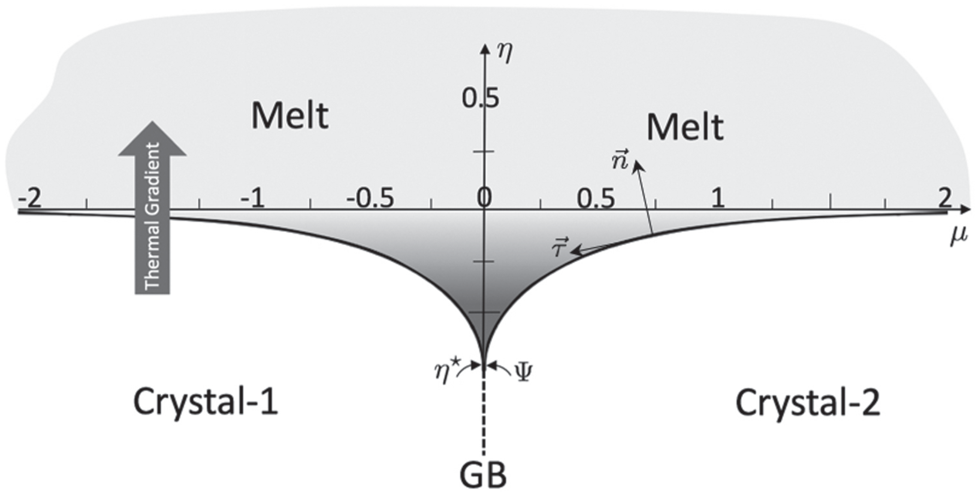
Figure 3.
Plot of the magnitudes of the capillary-mediated dimensionless fluxes, , along the left and right profiles of a grain boundary groove with zero dihedral angle. The directions of the -components of these fluxes oppose each other. Left and right thermal flux vectors rotate clockwise and anti-clockwise, respectively, as they descend into the steeper portion of the cusp. These components become parallel as the triple junction is approached, where their -components combine and enter the grain boundary with a flux magnitude of 8.
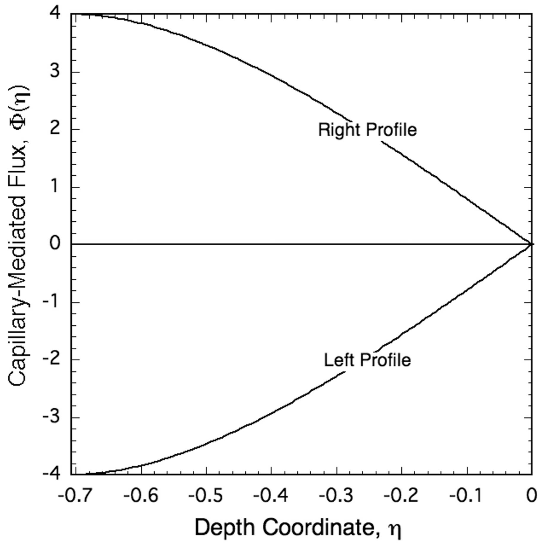
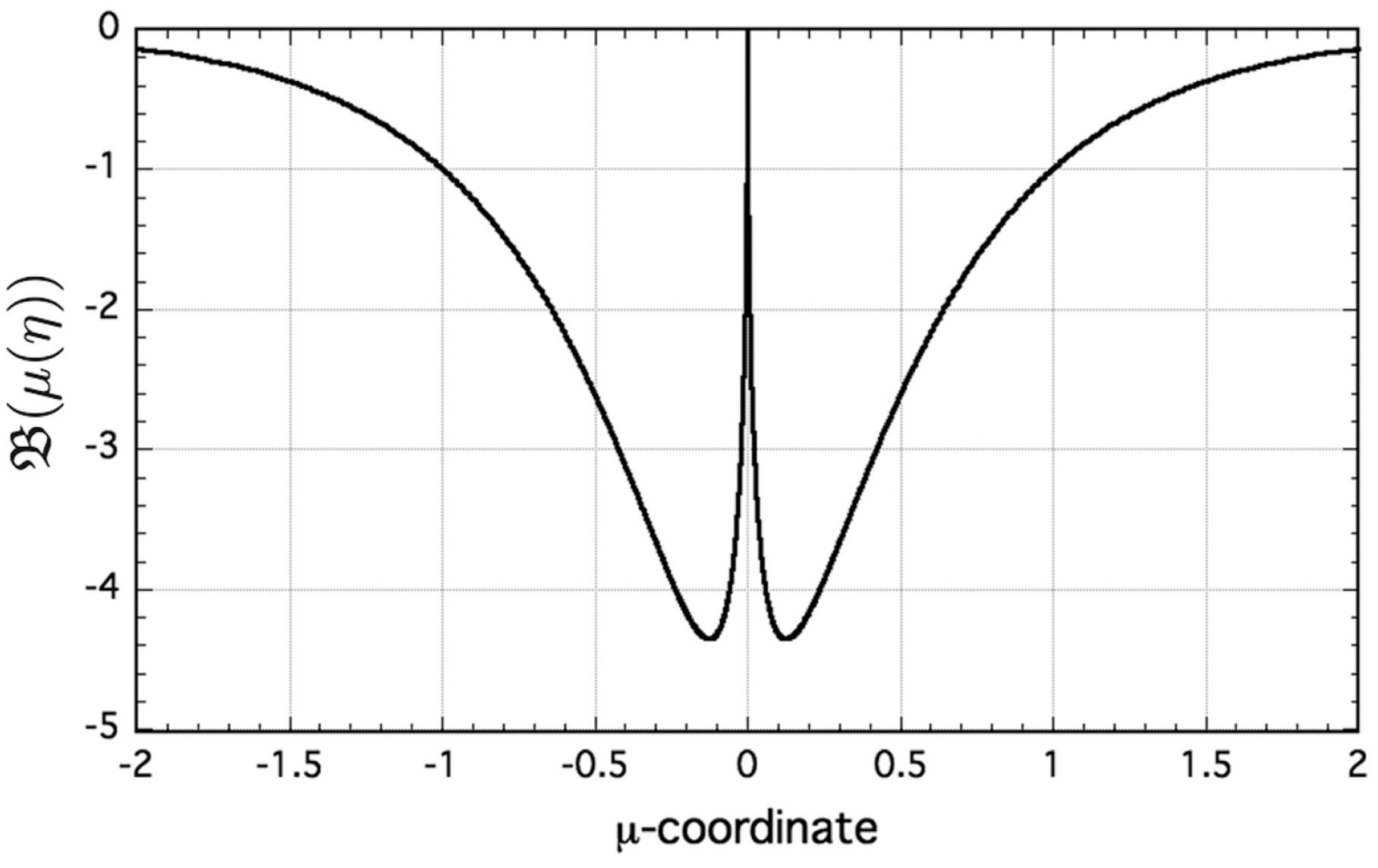
Figure 4.
Plot of capillary-mediated energy rates, (Equation (18)) for an equilibrated grain boundary groove with zero dihedral angle, specified by Equation (4). Energy rates are negative at all points along the groove’s solid–liquid interface, indicating that heat removal, i.e., cooling, occurs everywhere along the interface. The most intense cooling rate occurs at , roughly half-way between the groove’s triple junction at and the -axis, where .

Figure 5.
Theoretical cooling distribution for an equilibrated grain boundary groove with zero dihedral angle. Maximum cooling rates occur at . This unique distribution of capillary-mediated heat removal provides a robust target for independent verification, by comparing these theoretical cooling rates against those measured by direct equilibration of an equivalent grain boundary groove simulated using multiphase-field numerics.

Figure 6.
Phase-field residual potential measurements (⃝-symbols) along the simulated right isoline of an equilibrated grain boundary groove with zero dihedral angle. Data points plotted with the bias field distribution, , for its counterpart variational groove profile. The scale-factor 300:1 was chosen between the phase-field’s abscissa, -grid (minus 1000), and the dimensionless abscissa coordinate, . A fixed ratio, , applied to the left-ordinate is used here to compare simulated residuals () with the corresponding right-ordinate -distribution. The -value proportioning these simulation data was chosen as the ratio of the largest phase-field residual, , to the largest -value, . Residual measurements from phase-field simulation and the corresponding predicted distribution, , from sharp-interface theory represent independent estimates of capillary-mediated cooling perturbations along a stationary grain boundary groove.
© 2017 by the authors. Licensee MDPI, Basel, Switzerland. This article is an open access article distributed under the terms and conditions of the Creative Commons Attribution (CC BY) license (http://creativecommons.org/licenses/by/4.0/).
Share and Cite
MDPI and ACS Style
Glicksman, M.; Ankit, K. Detection of Capillary-Mediated Energy Fields on a Grain Boundary Groove: Solid–Liquid Interface Perturbations. Metals 2017, 7, 547. https://doi.org/10.3390/met7120547
AMA Style
Glicksman M, Ankit K. Detection of Capillary-Mediated Energy Fields on a Grain Boundary Groove: Solid–Liquid Interface Perturbations. Metals. 2017; 7(12):547. https://doi.org/10.3390/met7120547
Chicago/Turabian StyleGlicksman, Martin, and Kumar Ankit. 2017. "Detection of Capillary-Mediated Energy Fields on a Grain Boundary Groove: Solid–Liquid Interface Perturbations" Metals 7, no. 12: 547. https://doi.org/10.3390/met7120547
Note that from the first issue of 2016, this journal uses article numbers instead of page numbers. See further details here.