A Numerical Study on the Excitation of Guided Waves in Rectangular Plates Using Multiple Point Sources


1
Department of Mechanical, Aerospace and Civil Engineering, Brunel University London, Uxbridge, Middlesex UB8 3PH, UK
2
National Structural Integrity Research Centre, TWI Ltd, Cambridge CB21 6AL, UK
3
Department of Engineering Science, University of Greenwich, Chatham ME4 4TB, UK
*
Authors to whom correspondence should be addressed.
Metals 2017, 7(12), 552; https://doi.org/10.3390/met7120552
Submission received: 10 October 2017
/
Revised: 27 November 2017
/
Accepted: 29 November 2017
/
Published: 8 December 2017
(This article belongs to the Special Issue Advanced Non-Destructive Testing in Steels)
Abstract
:Ultrasonic guided waves are widely used to inspect and monitor the structural integrity of plates and plate-like structures, such as ship hulls and large storage-tank floors. Recently, ultrasonic guided waves have also been used to remove ice and fouling from ship hulls, wind-turbine blades and aeroplane wings. In these applications, the strength of the sound source must be high for scanning a large area, or to break the bond between ice, fouling and plate substrate. More than one transducer may be used to achieve maximum sound power output. However, multiple sources can interact with each other, and form a sound field in the structure with local constructive and destructive regions. Destructive regions are weak regions and shall be avoided. When multiple transducers are used it is important that they are arranged in a particular way so that the desired wave modes can be excited to cover the whole structure. The objective of this paper is to provide a theoretical basis for generating particular wave mode patterns in finite-width rectangular plates whose length is assumed to be infinitely long with respect to its width and thickness. The wave modes have displacements in both width and thickness directions, and are thus different from the classical Lamb-type wave modes. A two-dimensional semi-analytical finite element (SAFE) method was used to study dispersion characteristics and mode shapes in the plate up to ultrasonic frequencies. The modal analysis provided information on the generation of modes suitable for a particular application. The number of point sources and direction of loading for the excitation of a few representative modes was investigated. Based on the SAFE analysis, a standard finite element modelling package, Abaqus, was used to excite the designed modes in a three-dimensional plate. The generated wave patterns in Abaqus were then compared with mode shapes predicted in the SAFE model. Good agreement was observed between the intended modes calculated in SAFE and the actual, excited modes in Abaqus.
1. Introduction
Lamb waves are widely used to inspect the structural integrity of plates [1]. The plate is assumed to be infinitely long and infinitely wide, so that the sound field is considered to be uniform in the direction perpendicular to wave propagation. In practice, Lamb waves are used for plates whose width and length are large compared to the wavelength. In reality a plate is finite and the assumption of a constant sound field in one direction does not hold in all applications, especially in low-frequency applications where the wavelength is large compared to the dimensions. In this paper, the generation and propagation of wave modes in a three-dimensional plate is examined, where the sound field varies in both directions perpendicular to the wave-propagation direction. A semi-analytical finite-element (SAFE) method is developed to study guided wave modes. Modal shape, phase and energy velocities are extracted which provide information on which mode should be selected for non-destructive, de-icing or de-fouling applications. A number of point sources are used to generate a single wave mode that is propagating in the length direction only. The point sources are evenly distributed, and amplitudes of the point sources are determined by the mode shape. The generation and propagation of this mode is visualised with the commercial software package, Abaqus.
Dispersion equations for guided waves propagating in an infinite isotropic layer were first investigated by Rayleigh and Lamb [1,2]. The waveguide has very simple (two-dimensional) boundary conditions, i.e., one or two surfaces and no edges. Analytical and numerical solutions for these equations have been addressed by different authors [3]. In reality, a plate cannot be infinitely wide or long, however, when the thickness of the plate and wavelength of the guided wave are small compared to the other two dimensions Lamb wave theory can be used without considering interactions between waves and edges or defects. Lamb waves are widely adopted for non-destructive testing (NDT) of thin-wall plates [4,5,6]. For waveguides of other cross-section, such as cylinders, rectangular plates, rails, etc., modal solutions of the governing equations are more complicated due to the reflection of the waves from boundaries, and analytical solutions are thus often limited to simple geometries and/or fundamental modes [7,8,9,10,11,12]. Numerical solutions are attractive due to the flexibility of dealing with arbitrary geometry and complex boundary conditions. SAFE is one of the most popular numerical techniques for calculating the eigenmodes of guided waves in an arbitrary cross-sectional waveguide [13,14,15,16,17,18,19,20]. SAFE introduces analytical modal solutions into the wave equation, and requires only the cross-sectional area of the waveguide to be meshed.
For embedded or immersed waveguides, the cross-sectional area of the waveguide is infinite, but the conventional SAFE method cannot be used to model an infinite large area. In this case, SAFE can be used to model the inner layers of the waveguide, and the SAFE model is then coupled to other boundary models of the infinite surrounding layer, such as the perfectly matched layer (PML) method [21,22,23], the boundary element method (BEM) [24], the infinite element method [25], or the absorbing layer method [26]. In addition to SAFE, other numerical techniques are available for calculating the eigenmodes of guided waves, such as the BEM [27,28], the wave finite element method (WFE) [29,30,31,32] and the scaled boundary finite element method (SBFEM) [33,34,35,36]. BEM represents exactly the radiation boundary condition and reduces the dimensions of the numerical problem by one. However, this method has numerical stability problems and other mathematical challenges [24]. WFE meshes a small three-dimensional section of the waveguide, with a periodicity condition applied to both ends of the waveguide [29]. This method has the advantage of making use of commercially available finite element software packages. However, numerical round-off errors could appear when the axial wavelength (wavelength in the propagation direction) is small [32]. SBFEM also assumes harmonic wave solutions in the wave propagation direction, and thus discretises only the cross-sectional area of the waveguide for modal analysis. SBFEM can use higher order spectral elements to improve computation efficiency [34]; however, the discretisation of higher order elements cannot be generated using conventional meshing techniques, and element meshing can be difficult for complex geometries.
The above techniques are used to calculate the eigenmodes of guided waves. They assume the waveguide to be uniform in the wave propagation direction, but for wave scattering problems the waveguide is no longer uniform. In these cases the conventional finite element method can be used to model the whole waveguide and the length of the waveguide is often limited [37]. For a theoretically infinitely long waveguide, it is possible to combine a modal expansion solution with a conventional finite element solution, requiring only a small non-uniform section of the waveguide to be meshed [38,39,40,41]. SBFEM is also an efficient alternative, which requires only the boundary of the waveguide to be meshed [42].
This paper studies the excitation of well-designed guided waves in a rectangular plate. The number of modes that could propagate in a waveguide are indicated by the dispersion curves which, however, do not reveal how to excite a particular mode using a finite number of point sources. Early work on the study of guided waves in rectangular plates was limited to extensional wave modes associated with two dimensions of the plate [43]. Standing wave patterns were generated to observe wavelengths and associated wave velocities at different frequencies. Recently, Cegla studied the excitation of two modes having modal energy focused at the centre of the plate [44]. One of these modes was a shear horizontal type mode, and the other was a flexural type mode. To excite these modes, the profile of the excitation force should resemble the mode profile as closely as possible. However, it is not possible to experimentally implement these mode profiles with a continuous excitation profile over the cross-sectional area of the plate. Instead, individual transducers are used which cover only part of the cross-sectional area. The excitation of the two modes (shear and flexural) was achieved by placing a transducer at the centre of the end of the plate. Furthermore, these two modes are both strongest at the centre of the plate and the modal energy decreases towards the edge.
The number of excited wave modes for rectangular plates in these reference papers is very limited, and the potential application of other guided wave modes has not been exploited in the literature. This paper thus proposes a method to systematically excite three types of guided wave modes (shear-horizontal, flexural and extensional) and Rayleigh surface waves in a rectangular plate. These wave modes are relatively non-dispersive, and have the potential to propagate over long distances. Furthermore, they are designed to cover different areas of the plate, and have a dominant displacement in different directions. A combination of these modes can be used to cover the whole plate for NDT, de-icing or de-fouling applications. The remainder of the paper is structured as follows: the theoretical basis of the semi-analytical finite element method is presented in Section 2; dispersion curves and modal analysis are presented in Section 3; the excitation of a number of modes is presented in Section 4; and conclusions are drawn in Section 5.
2. Semi-Analytical Finite-Element Method
A large aspect ratio (width/thickness) rectangular plate is considered. The SAFE technique meshes only the cross-sectional area of the waveguide. The governing equation for wave propagation in an elastic medium is given by Navier’s Equation (1) [39]:
where and are the Lamé constants, is the displacement vector, is density and is time. A time dependence of is assumed, where is the radian frequency and . The displacement vector can be decomposed as , and in the x, y and z directions, respectively. On the surface of the plate it is assumed that no external forces are present so that all the tractions over the surface are zero.
The displacements in the cross-sectional area of the plate are expanded as a sum of eigenmodes to give:
where the subscript , and are the eigenvectors, with so that is a dimensionless wavenumber. In addition, and are the shear (transverse) and compressional (longitudinal) bulk-wave velocities, respectively.
The finite-element analysis proceeds by discretising the displacements of any mode over the plate cross-section. Equation (2) is then substituted back into Equation (1) and, by using a weak formulation and introducing the boundary conditions, one may arrive at the following general eigen Equation (3):
where . The constituents of matrices and are given in [39] and are not reproduced here.
3. Dispersion Curves and Modal Analysis
The eigen solution Equation (3) was programmed in MATLAB (R2017a, The MathWorks, Inc., Natick, MA, USA) and executed on a laptop with a 2.60 GHz Intel Core™ CPU and a 16 GB RAM. It has been shown that SAFE is able to deliver accurate solutions for dispersion curves in pipes [39]. The accuracy of the model for a rectangular plate is further examined here. The dispersion curves for a nickel plate are calculated and compared to the dispersion curves shown in ‘Figure 4a’ of Mukdadi et al.’s paper [13]. The thickness and width of the plate is 0.11 mm and 0.88 mm respectively. Material properties of the nickel plate can be represented as , , and [13]. Mukdadi et al. [13] used a variational principle to solve the governing equations. Analytical modal solutions were used in the wave propagation direction as well. A more general, weighted residual method is used in this paper. In principle, these two methods should deliver identical solutions, and this is shown in Figure 1 where the two numerical solutions match very well. Only a few low order modes are presented in Figure 1 for clarity, and this shows that SAFE is able to accurately calculate dispersion curves for rectangular plates. Note that SAFE is also able to calculate dispersion curves for Lamb waves in an infinitely wide plate. This can be done by setting displacements in the width direction to be constant. A number of additional convergence studies for plates have been carried out, and details are not shown here for the sake of space. Further validation of the SAFE model can be found in [39].
The dispersion curves shown above are for a small plate of thickness 0.11 mm. In NDT applications the plate could be much larger than that studied in Figure 1. A large rectangular steel plate is thus examined in the following sections of the paper, with a plate thickness of 10 mm, width of 400 mm, and length of 1.5 m. The aspect ratio (width/thickness) is thus 40. The purpose of the modal analysis here is not only to derive the dispersion curves, but to demonstrate which modes are suitable for NDT applications, and also how to excite selected modes. The properties of the steel plate are , , . Eight-node quadratic elements are used to mesh the cross-sectional area of the plate, with an element size of 2 mm. This ensures at least 32 nodes per wavelength for the shortest bulk wave up to 100 kHz. This level of element density is higher than that seen in conventional finite-element models, and this is to ensure that flexural modes (modes with displacement variations in the thickness direction of the plate) are captured accurately. The total number of degrees of freedom is 10,233, and the calculation took about 1 s to solve at each frequency.
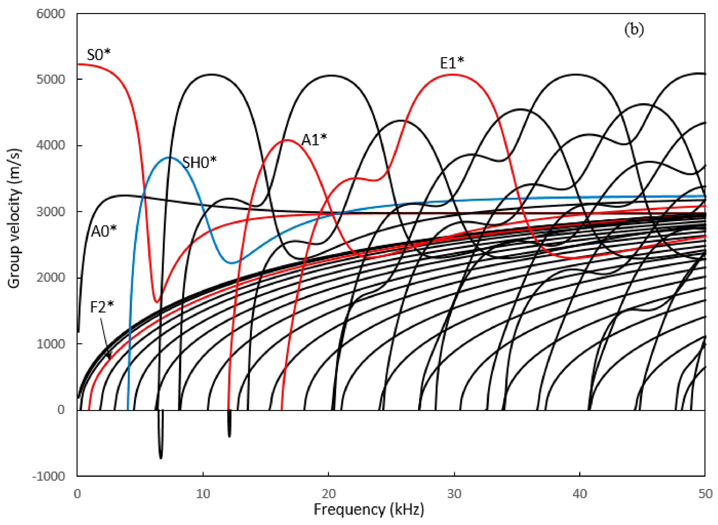
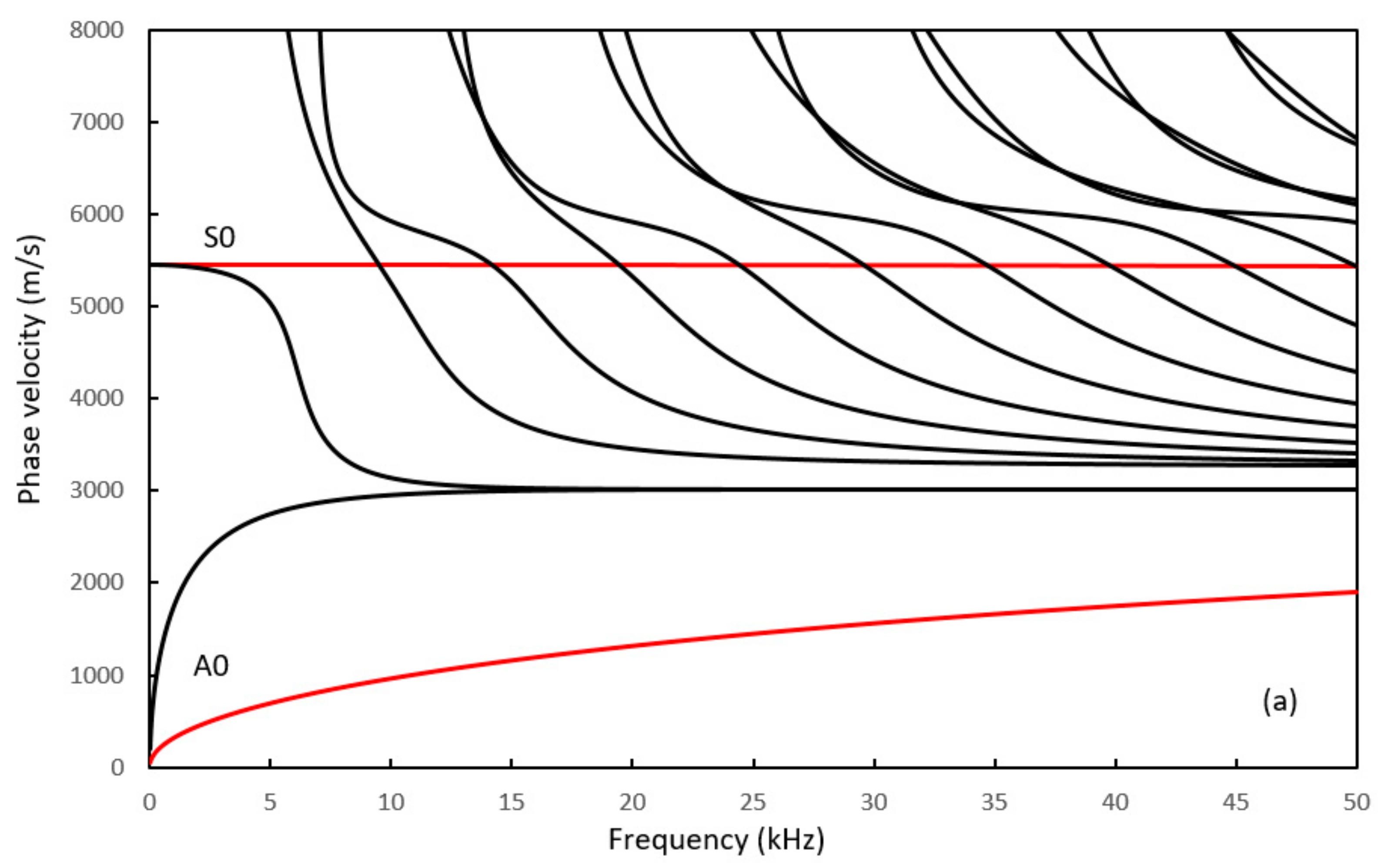
Figure 2 shows phase and group velocities for guided waves propagating in the rectangular plate. Dispersion curves for Lamb waves propagating in an infinite plate with a thickness of 10 mm and 400 mm are shown in Figure 3 for comparison. The dispersion curves are shown up to 50 kHz for clarity. Guided wave modes in the rectangular plate are different to Lamb wave modes in that these waves are reflected by four surfaces, rather than two. The number of wave modes is also much larger than corresponding Lamb-type wave modes. Backward waves can also be seen in Figure 2b with negative group velocities [45,46]. These waves are highly dispersive. For NDT applications, the incident mode is required to propagate as far as possible, and thus dispersive modes are normally avoided. Figure 2 shows that none of the modes has a constant velocity throughout the frequency range. However, it is possible to select a few modes that have a relatively uniform velocity distribution in a particular frequency band and these are marked in colour in Figure 2, and investigated further in this paper. The SH0* mode indicates a shear horizontal type mode with dominant displacement in the width direction of the plate. However, the displacement is not constant because the wave is reflected by surfaces. The superscript * is thus used to indicate that SH0* is different to the conventional shear-horizontal mode in an infinitely large plate where displacement is constant in the width direction. S0* and A0* modes are symmetric and anti-symmetric modes, respectively, along the width direction of the plate. As frequency increases, the wavelength of these modes decreases. They become Rayleigh waves in the high frequency range, where modal energy focuses near the edge of the plate. The detailed modal analysis of these and other modes is presented in the next section associated with their visualisation in the three-dimensional plate.
4. Excitation of Guided Wave Modes
A large number of wave modes could exist at a single frequency. It is thus difficult to excite a pure single wave mode. A general principle is that the loading profile should match the profile of the wave mode to be excited. However, each mode has a displacement distribution that is continuous across the cross-sectional area of the plate. In practice, the loading profile can only be controlled by individual discrete transducers, and it is not possible to generate a continuous loading profile over the plate transverse plane. For a large plate, such as the one studied here, it is more appropriate to represent each transducer as a point source. The aim is then to use a finite number of point sources to excite a particular wave mode. In this case, the loading profile is discrete, rather than continuous.
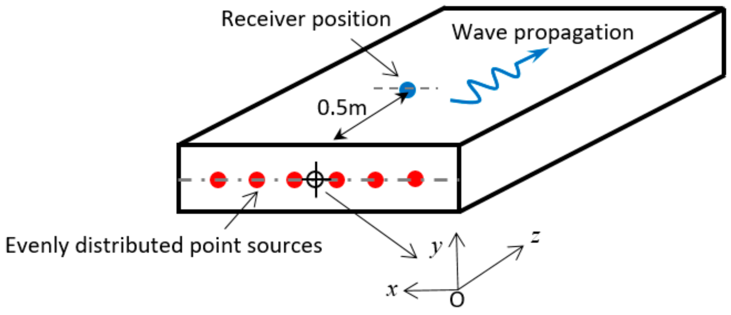
A commercial finite element software package, Abaqus (version 6.14-4, Dassault Systèmes Americas Corp., Waltham, MA, USA), has been used to visualise and validate this method. The plate has a thickness of 10 mm, width of 400 mm, and length of 1.5 m. The point sources are evenly distributed, and placed at the centre of the plate end (y = 0 and z = 0, see Figure 4). The edges between two surfaces have surface normals perpendicular to each other. This produces normal stress singularity lines and so no excitation point sources are placed on the edges of the plate. Suppose the number of point sources used for excitation of a particular mode is N, then the interval between adjacent point sources will be 400/(N + 1) mm, where 400 mm is the width of the plate. Thus the position of each source can be easily calculated based on the number of total point sources. The number of point sources, and the amplitude of each point source needed to excite a single mode are determined by the mode shape. The absolute amplitude of all the point sources could be increased or decreased proportionally; however, the relative amplitude of these point sources shall resemble the mode shape of the mode to be excited. For different wave modes, the direction of the loading displacement is also different. This depends on the direction of the dominant displacement seen from the mode shape. The details of these point sources will be presented in Section 4.1–Section 4.4. Rayleigh waves and three other types of waves are studied, i.e., shear type (dominant in x direction), flexural type (dominant in y direction) and extensional type (dominant in z direction).
The Abaqus Explicit module was used to produce a transient wave field. The incident signal is a 10-cycle Hanning-windowed pulse. Isoparametric linear hexahedral elements were used. The element size is 5 mm in the x and z directions. In the y direction (thickness), the element size is reduced to 0.5 mm in order to capture displacement variations for high order modes. The total number of elements is 480,000, taking around 35 min to solve for each excitation. The displacement distribution for the three-dimensional plate can be shown in the form of a colour map in the post-processing stage. The detailed wave propagation form at a particular receiver position can also be shown as a function of time. The longitudinal receiver position is fixed to be 0.5 m from the edge of the plate (see Figure 4). The transverse position (x width direction) of the receiver is associated with the peak amplitude of each mode and is thus mode dependent.
4.1. Excitation of Rayleigh Modes
The S0* and A0* modes shown in Figure 2 are fundamental Lamb type modes associated with the width (400 mm side) of the plate in the low frequency range below 5 kHz. These two modes become almost non-dispersive in the high frequency range above 20 kHz. However, Rayleigh waves are surface waves with energy focused near the edge of the plate, and so these modes can only detect defects near the edge of the plate. Figure 5 shows the mode shape of S0* at 50 kHz. This mode has a dominant shear displacement near the edge of the plate. The extensional displacement is slightly smaller than the shear displacement. The vertical displacement is very small and can be ignored.
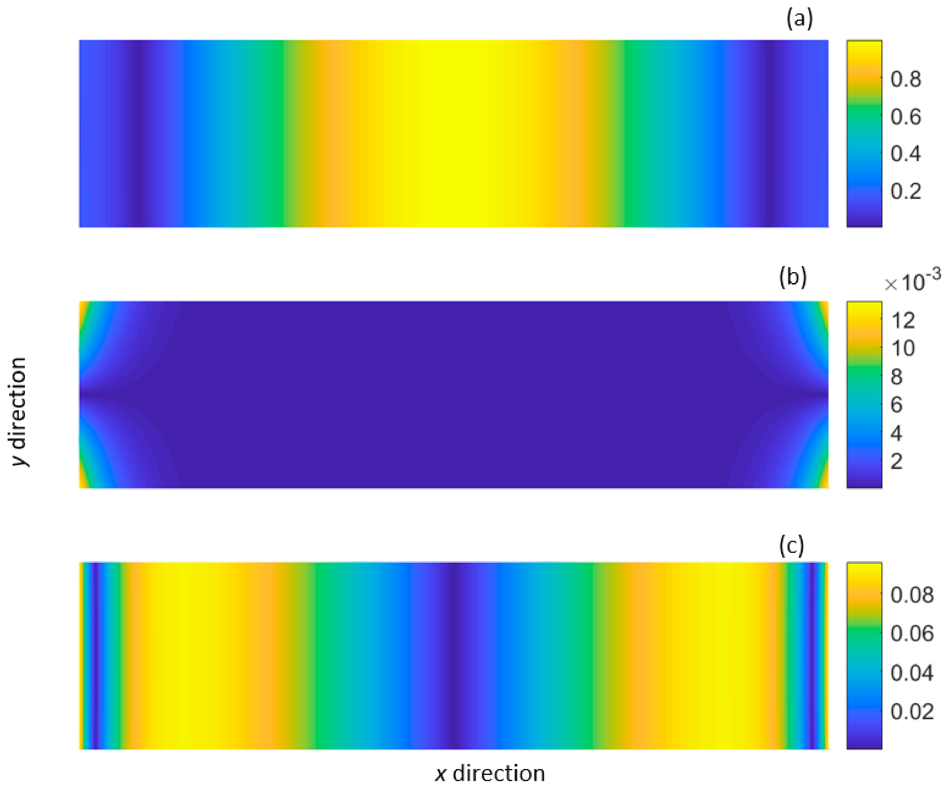
A number of discretised point sources along the centre line of the plate (shown in Figure 4) is proposed to excite this mode. The amplitude of point sources is determined by the mode shape shown in Figure 5. The shear and extensional displacements along the centre line of the plate are extracted from Figure 5a,c and represented in Figure 6a,b. Note that colour maps shown in Figure 5a,c are based on absolute displacement amplitude, while Figure 6a,b incorporate phase variations so that positive and negative displacements are presented. Further details on the amplitude of point sources and excitation of this wave mode will be presented in Figure 6.
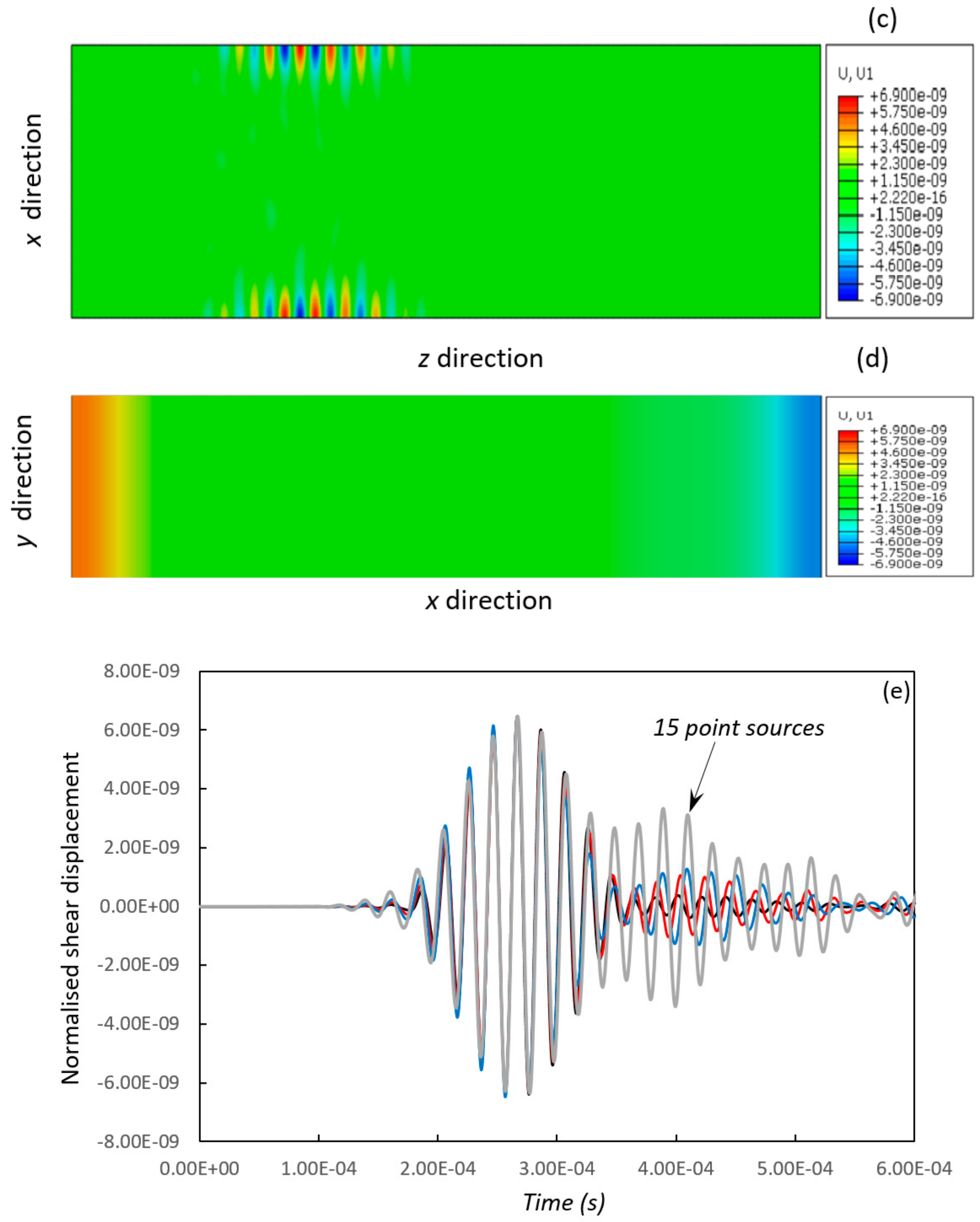
Rayleigh wave S0* has displacements focused near the edge of the plate. The simplest way to excite this wave mode is to try to place a single transducer on the edge of the plate. This would indeed generate S0*; however, other compressional and shearing type waves will be generated as well. To excite a pure Rayleigh S0* mode, a series of numerical experiments were conducted by varying the number of sources and the direction of the excitation displacement. The generated mode shape was presented in Figure 6c,d and then compared to the predicted mode shape shown in Figure 5. It was found that S0* could be excited by applying the shear-displacement loading at a number of point sources; however, a noise region would appear behind the S0* wave mode. This noise region could be significantly reduced by applying both shear and extensional displacements at each point source. This is because the extensional displacement is comparable to the shear displacement, and elimination of the extensional displacement would produce additional noise. Furthermore, the extensional and the shear displacement have a phase difference of 90°. This corresponds to a quarter of a period at 50 kHz in the time domain with the extensional displacement leading the shear displacement. In the Abaqus module, both shear and extensional displacements were assigned to each point source in the loading stage. The number of point sources was gradually reduced from 79 to 3.
Figure 6a,b show the profile of the loading displacement calculated from SAFE. The generated wave propagation displacement from Abaqus is presented in Figure 6c–e. The incident wave is centred at 50 kHz. Figure 6a,b is used to determine the amplitude of the loading at each point source in Abaqus. The solid lines in Figure 6a,b is displacement amplitude obtained from SAFE. The shear displacement is evenly sampled in Figure 6a and the amplitude associated with each location is used as the amplitude of the corresponding point source in Abaqus. The extensional displacement in Figure 6b is evenly sampled in the same way. Note that the amplitudes shown in Figure 6a,b are normalized relative amplitudes between point sources. In Abaqus, these normalized amplitudes are multiplied by a constant 10−8, so that displacements have the unit of meter in Abaqus. It can be seen that both shear and extensional displacements of this mode drop almost exponentially from the edge of the plate towards the centre in the width direction (see Figure 6a,b). The point sources from x = −50 mm to x = 50 mm play a minimal role and could be discarded in actual applications. The distance between adjacent point sources should be small to capture the rapid drop of displacements near the edge of the plate (x → −200 mm or 200 mm).
The generated wave will start to propagate from z = 0 towards the far end of the plate z = 1.5 m. The displacement distribution of the generated wave will be a function of both position and time. To verify that the generated wave is indeed the designed wave mode, the generated wave propagation form has been observed in different ways, shown in Figure 6c–e. Figure 6c,d is top and transverse view of the plate at a fixed time, and Figure 6e is the time-domain wave propagation form at a fixed position. Wave speed and mode shape are compared with each other. The intended wave mode has a group velocity of 2979.5 m/s, and the wave speed of the generated wave mode is calculated to be 2978.6 m/s. The difference in terms of wave speed is less than 0.1%. The shear displacement of the intended wave mode is shown in Figure 5a, and this can be compared to the shear displacement of the generated wave mode shown in Figure 6d. It can be seen that the two figures match each other very well, considering phase variation and the symmetric nature of this mode. In addition to the shear displacement, the intended and generated extensional displacement distribution have also been compared and they match each other very well.
Figure 6c,d is generated wave distribution from 79 point sources, and it is clear that a single pure Rayleigh wave has been generated which propagates near the edges of the plate. Figure 6e compares the received time-domain wave forms from a varying number of point sources. As the number of sources decreases, the distance between adjacent point sources increases. The discretised loading displacement profile starts to deviate from the continuous displacement profile, and the noise level increases. When 15 point sources are used, the Rayleigh wave has been significantly influenced by other shearing waves from individual point sources.
4.2. Excitation of Shear Type Modes
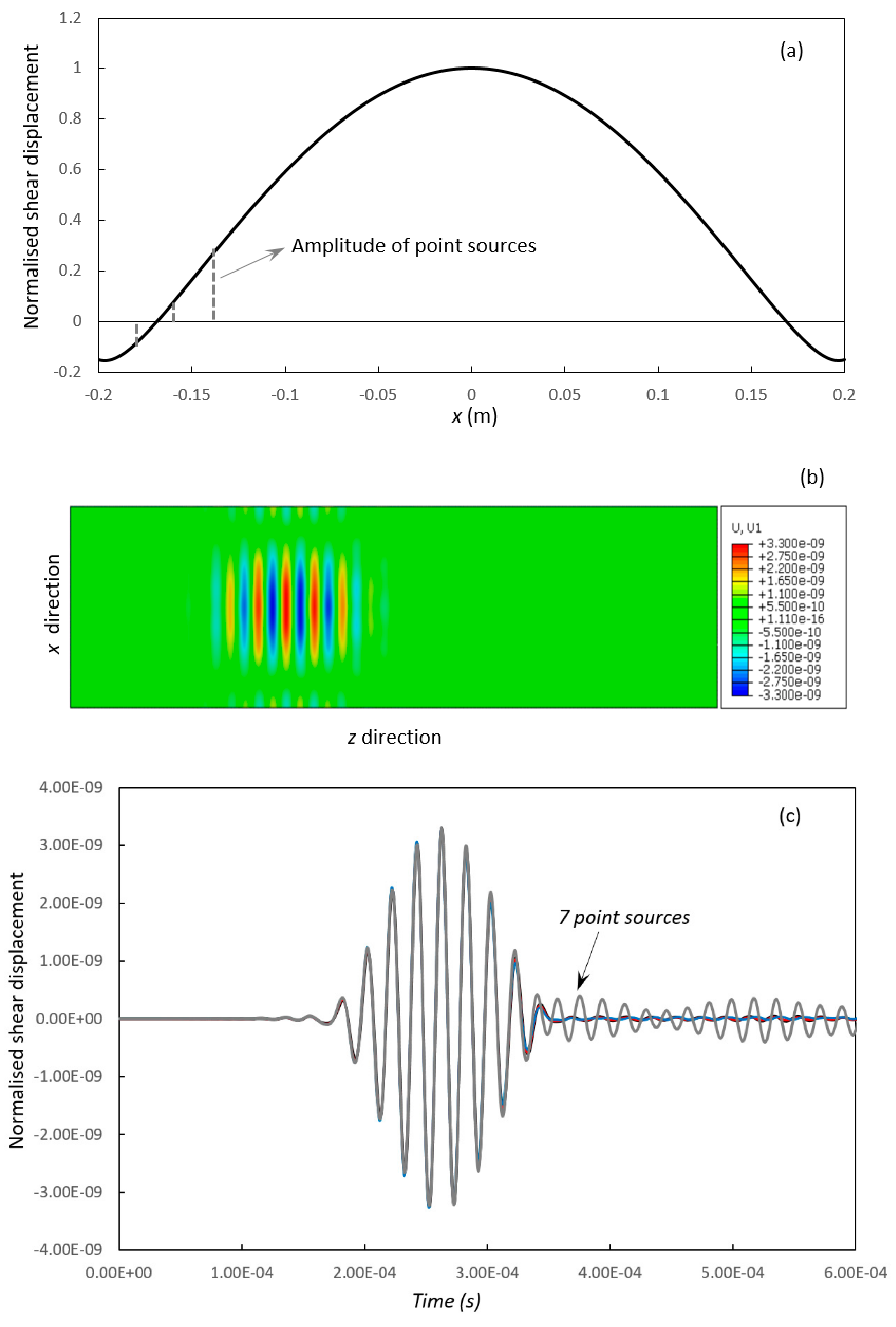
The first shear type mode to be examined is the shear-horizontal type SH0* mode. This mode has a dominant shear displacement, and the shear displacement is strongest near the centre of the plate. Figure 7 shows the modal shape of this mode at 50 kHz. Cegla [44] showed that a continuous excitation profile is able to generate this mode at 2 MHz. In Cegla’s experiment, a single transducer was used to cover most area of the transverse plane of the plate, and the experimental excitation profile approaches the theoretical continuous excitation profile. However, the plate and wavelength studied here is much larger than those studied in [44], and it is more appropriate to represent each transducer as an individual point source. To generate this mode, it was found that the excitation displacement needs to be pointed in the shear (x) direction only. This mode is thus much easier to excite than the Rayleigh mode S0*.
Figure 8a shows the shear displacement excitation profile from SAFE. This profile is discretised and point sources are used to generated SH0* in Abaqus in the loading stage. The shear displacement falls smoothly from the centre of the plate towards the edge, and the number of point sources used to capture this mode is relatively small compared to S0*. Figure 8b shows the generated shear-displacement distribution profile from 19 point sources, and a single pure SH0* mode has been generated which propagates at the centre of the plate. Figure 8c compares the received time domain displacements excited by different numbers of point sources. Now, 9 point sources are enough to generate a pure SH0* mode with negligible noise. The noise level increases slightly when only 7 point sources are used.
Figure 9 shows the excitation of another shear type mode, A1*. The dispersion curves for this mode are given in Figure 2. It can be seen that this mode has relatively flat velocity curves near 50 kHz. The two-dimensional shape of this mode is not presented here for the sake of space, however its shear displacement is shown in Figure 9a, and the generated displacement distribution profile is shown in Figure 9b. This mode has positive and negative peaks in the width (x) direction. Figure 9c shows that 9 point sources are enough to excite the mode with negligible noise. The noise starts to appear when 7 or fewer point sources are used.
4.3. Excitation of Extensional Type Modes
Figure 10 shows the mode shape of an extensional type mode E1* at 30 kHz. This mode is generally dispersive; however, in a narrow region near 30 kHz, it has relatively flat velocity curves (see Figure 2). Along the width direction of the plate there is a dominant extensional displacement with four peak regions. The trough displacement, however, is not zero with a minimal extensional displacement of around 42% of the maximum. This means that this mode can be used to cover the entire plate without any blind regions, which is an attractive property.
Figure 11a shows the extensional displacement distribution along the centre line of the plate, which is discretised and then used at the loading stage in the Abaqus model. Figure 11b,c show the displacement distribution generated in Abaqus. A single mode wave pattern can be seen clearly in Figure 11b with 19 evenly distributed point sources. The number of point sources can be further reduced, and the noise level is still low when only 7 sources are used. The noise level increases significantly when 3 point sources are used. Note that a number of other extensional modes have relatively flat dispersion curves but are not reported here for the sake of space.
4.4. Excitation of Flexural Type Modes
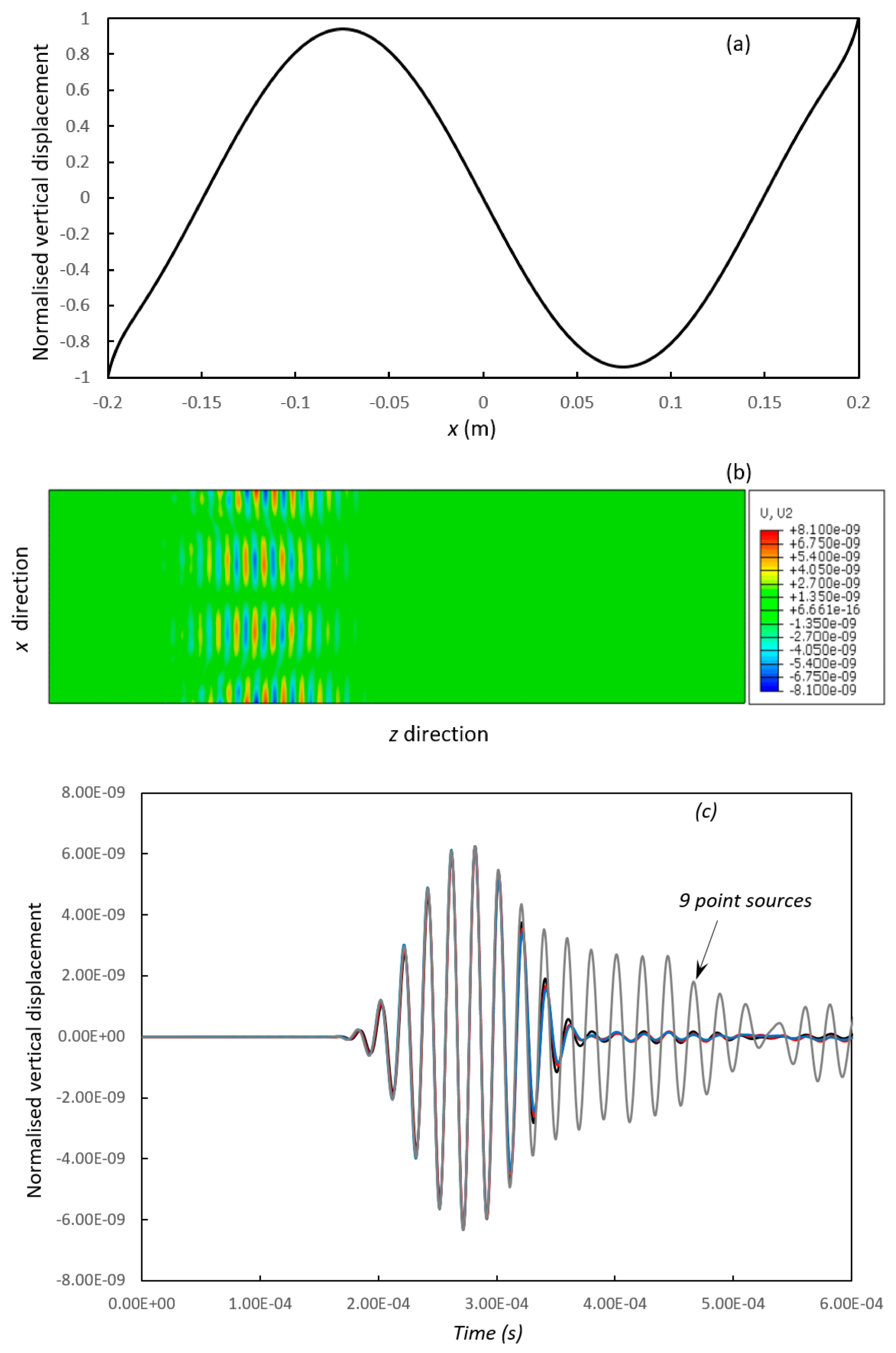
In this section, a flexural type mode, F2* is examined that has a dominant vertical (y direction) displacement. The dispersion curves are shown in Figure 2. It can be seen that F2* is generally dispersive, especially in the low frequency range. The mode shape of F2* at 50 kHz is shown in Figure 12. This frequency is chosen because the dispersion curves are relatively flat here. The shear displacement is negligible, and the extensional displacement is relatively strong only near the surface of the plate.
The vertical displacement (flexural type displacement that vibrates up and down in the thickness direction) along the centre of the plate is discretised to excite this mode in Figure 13. It has four antinodal positions along the width of the plate. It can be seen that a single F2* mode can be excited by 15 or more evenly distributed point sources. The noise level increases significantly when 9 point sources are used. Note that other flexural type modes have been excited here but are not described.
5. Conclusions
In this paper, a two-dimensional, semi-analytical finite element method is used to study the dispersion curves and mode shapes of wave modes in a rectangular plate. These waves are different to Lamb waves in that guided waves are bounded by four surfaces and propagate in only a single direction. All the wave modes have displacements in three directions of the plate; however, each has a dominant displacement in a single direction. According to the dominant displacement, wave modes can be classified into four categories: Rayleigh surface waves, shear waves, extensional waves and flexural waves. This paper studies the excitation of a single wave mode by a set of evenly distributed point sources. The four types of wave modes are all discussed in this paper, and their excitation is visualised in Abaqus.
For simple and systematic presentation, all the point sources are distributed evenly along the horizontal centre line of the plate. It was found that a single wave mode can be generated by a finite number of point sources. The number of point sources required to generate a single mode is related to the wave shape of the mode. The surface wave S0* has a displacement that decays almost exponentially along the width direction of the plate, and a large number of point sources are required to excite this mode accurately. Furthermore, this mode has comparable displacements in both the shear and extensional directions, and it was found that the quality of the signal could be improved by applying shear and extensional displacement loading at each point source. This two-directional excitation method may be difficult to implement in reality, and practical implementation of this method requires further investigation. However, all the other three types of wave modes require excitation displacement to be applied in only one direction.
The modes studied in this paper were chosen by the relative flatness of their dispersion curves, so that they can propagate far. They have dominant displacements in different directions, which could be used in different applications. For instance, Palacios et al. used ultrasonic actuators to instantaneously delaminate the ice layer from a steel substrate [47]. This required the shear stress between the two layers to exceed a certain value, and this was achieved at resonance frequencies where the ultrasonic actuators provided maximum current outputs for a given driving voltage. Localized stress-concentration areas could be observed when one or two actuators were used. The research carried out here could potentially benefit these applications by improving stress-concentration areas. A number of modes studied here have not previously been investigated. For example, the extensional type E1* mode has extensional displacement along the entire width of the plate without nodal positions. Its minimal extensional displacement is above 40% of the maximum and could thus be used to cover the whole plate. The practical application of this and other modes reported in this paper will be under further investigation.
Author Contributions
Wenbo Duan carried out the semi-analytical finite element method and initiated the concept to excite intended wave modes; Xudong Niu implemented the three dimensional numerical analysis in Abaqus; Wenbo Duan and Tat-Hean Gan contributed to the drafting of the manuscript; Jamil Kanfoud and Hua-Peng Chen supervised the work reported in this paper.
Conflicts of Interest
The authors declare no conflict of interest.
References
- Lamb, H. On Waves in an Elastic Plate. Proc. R. Soc. Lond. Ser. A 1917, 93, 114–128. [Google Scholar] [CrossRef]
- Rayleigh, L. On the free vibrations of an infinite plate of homogeneous isotropic elastic matter. Proc. Lond. Math. Soc. 1889, 20, 225–234. [Google Scholar] [CrossRef]
- Meleshko, V.V.; Bondarenko, A.A.; Dovgiy, S.A.; Trofimchuk, A.N.; van Heijst, G.J.F. Elastic waveguides: History and the state of the art. I. J. Math. Sci. 2009, 162, 99–120. [Google Scholar] [CrossRef]
- Diligent, O. Interaction between Fundamental Lamb Modes and Defects in Plates. Ph.D. Thesis, Mechanical Engineering Department, Imperial College London, London, UK, 2003. [Google Scholar]
- Lee, B.C.; Staszewski, W.J. Lamb Wave Propagation modelling for damage detection: I. Two-dimensional analysis. Smart Mater. Struct. 2007, 16, 249–259. [Google Scholar] [CrossRef]
- Burrows, S.E.; Dutton, B.; Dixon, S. Laser generation of Lamb waves for defect detection: Experimental methods and finite element modelling. IEEE Trans. Ultrason. Ferroelectr. Freq. Control 2012, 59, 82–89. [Google Scholar] [CrossRef] [PubMed]
- Mindlin, R.D.; Fox, E.A. Vibrations and waves in elastic bars of rectangular cross section. Trans. ASME J. Appl. Mech. 1960, 27, 152–158. [Google Scholar] [CrossRef]
- Medick, M.A. Extensional waves in elastic bars of rectangular cross section. J. Acoust. Soc. Am. 1968, 43, 152–161. [Google Scholar] [CrossRef]
- Kastrzhitskaya, E.V.; Meleshko, V.V. Propagation of harmonic waves in an elastic rectangular waveguide. Sov. Appl. Mech. 1990, 26, 773–781. [Google Scholar] [CrossRef]
- Lowe, M.J.S. Matrix techniques for modelling ultrasonic waves in multi-layered media. IEEE Trans. Ultrason. Ferroelectr. Freq. Control 1995, 47, 525–542. [Google Scholar] [CrossRef]
- Krushynska, A.A.; Meleshko, V.V. Normal waves in elastic bars of rectangular cross section. J. Acoust. Soc. Am. 2011, 129, 1324–1335. [Google Scholar] [CrossRef] [PubMed]
- Kuo, C.W.; Suh, C.S. On the dispersion and attenuation of guided waves in tubular section with multi-layered viscoelastic coating—Part I: Axial wave propagation. Int. J. Appl. Mech. 2017, 9, 1750001. [Google Scholar] [CrossRef]
- Mukdadi, O.M.; Desai, Y.M.; Datta, S.K.; Shah, A.H.; Niklasson, A.J. Elastic guided waves in a layered plate with rectangular cross section. J. Acoust. Soc. Am. 2002, 112, 1766–1779. [Google Scholar] [CrossRef] [PubMed]
- Hayashi, T.; Song, W.J.; Rose, J.L. Guided wave dispersion curves for a bar with an arbitrary cross-section, a rod and rail example. Ultrasonics 2003, 41, 175–183. [Google Scholar] [CrossRef]
- Bartoli, I.; Marzani, A.; Lanza di Scalea, F.; Viola, E. Modeling wave propagation in damped waveguides of arbitrary cross-section. J. Sound Vib. 2006, 295, 685–707. [Google Scholar] [CrossRef]
- Mu, J.; Rose, J.L. Guided wave propagation and mode differentiation in hollow cylinders with viscoelastic coatings. J. Acoust. Soc. Am. 2008, 124, 866–874. [Google Scholar] [CrossRef] [PubMed]
- Treyssède, F. Elastic waves in helical waveguides. Wave Motion 2008, 45, 457–470. [Google Scholar] [CrossRef]
- Treyssède, F.; Laguerre, L. Investigation of elastic modes propagating in multi-wire helical waveguides. J. Sound Vib. 2010, 329, 1702–1716. [Google Scholar] [CrossRef]
- Mazzotti, M.; Marzani, A.; Bartoli, I.; Viola, E. Guided waves dispersion analysis for prestressed viscoelastic waveguides by means of the SAFE method. Int. J. Solids Struct. 2012, 49, 2359–2372. [Google Scholar] [CrossRef]
- Treyssède, F. Dispersion curve veering of longitudinal guided waves propagating inside prestressed seven-wire strands. J. Sound Vib. 2016, 367, 56–68. [Google Scholar] [CrossRef]
- Nguyen, K.L.; Treyssède, F.; Hazard, C. Numerical modeling of three-dimensional open elastic waveguides combining semi-analytical finite element and perfectly matched layer methods. J. Sound Vib. 2015, 344, 158–178. [Google Scholar] [CrossRef]
- Duan, W.; Kirby, R.; Mudge, P.; Gan, T.-H. A one dimensional numerical approach for computing the eigenmodes of elastic waves in buried pipelines. J. Sound Vib. 2016, 384, 177–193. [Google Scholar] [CrossRef]
- Zuo, P.; Fan, Z. SAFE-PML approach for modal study of waveguides with arbitrary cross sections immersed in inviscid fluid. J. Sound Vib. 2017, 406, 181–196. [Google Scholar] [CrossRef]
- Mazzotti, M.; Bartoli, I.; Marzani, A.; Viola, E. A coupled SAFE-2.5D BEM approach for the dispersion analysis of damped leaky guided waves in embedded waveguides of arbitrary cross-section. Ultrasonics 2013, 53, 1227–1241. [Google Scholar] [CrossRef] [PubMed]
- Hua, J.; Mu, J.; Rose, J.L. Guided wave propagation in single and double layer hollow cylinders embedded in infinite media. J. Acoust. Soc. Am. 2011, 129, 691–700. [Google Scholar]
- Castaings, M.; Lowe, M. Finite element model for waves guided along solid systems of arbitrary section coupled to infinite solid media. J. Acoust. Soc. Am. 2008, 123, 696–708. [Google Scholar] [CrossRef] [PubMed]
- Gunawan, A.; Hirose, S. Boundary element analysis of guided waves in a bar with an arbitrary cross-section. Eng. Anal. Bound. Elem. 2005, 29, 913–924. [Google Scholar] [CrossRef]
- Mazzotti, M.; Bartoli, I.; Marzani, A.; Viola, E. A 2.5D boundary element formulation for modeling damped waves in arbitrary cross-section waveguides and cavities. J. Comput. Phys. 2013, 248, 363–382. [Google Scholar] [CrossRef]
- Mace, B.R.; Duhamel, D.; Brennan, M.J.; Hinke, L. Finite element prediction of wave motion in structural waveguides. J. Acoust. Soc. Am. 2005, 117, 2835–2843. [Google Scholar] [CrossRef] [PubMed]
- Mace, B.R.; Manconi, E. Modelling Wave Propagation in Two-Dimensional Structures Using Finite Element Analysis. J. Sound Vib. 2008, 318, 884–902. [Google Scholar] [CrossRef]
- Maki, Y.; Mace, B.R.; Brennan, M.J. Numerical issues concerning the wave and finite element method for free and forced vibrations of waveguides. J. Sound Vib. 2009, 327, 92–108. [Google Scholar]
- Søe-Knudesn, A.; Sorokin, S. On accuracy of the wave finite element predictions of wavenumbers and power flow: A benchmark problem. J. Sound Vib. 2011, 330, 2694–2700. [Google Scholar] [CrossRef]
- Song, C. The scaled boundary finite element method in structural dynamics. Int. J. Numer. Methods Eng. 2009, 77, 1139–1171. [Google Scholar] [CrossRef]
- Gravenkamp, H.; Man, H.; Song, C.; Prager, J. The computation of dispersion relations for three-dimensional elastic waveguides using the Scaled Boundary Finite Element Method. J. Sound Vib. 2013, 332, 3756–3771. [Google Scholar] [CrossRef]
- Gravenkamp, H.; Birk, C.; Song, C. Computation of dispersion curves for embedded waveguides using dashpot boundary condition. J. Acoust. Soc. Am. 2014, 135, 1127–1138. [Google Scholar] [CrossRef] [PubMed]
- Gravenkamp, H.; Birk, C.; Van, J. Modeling ultrasonic waves in elastic waveguides of arbitrary cross-section embedded in infinite solid medium. Comput. Struct. 2015, 149, 61–71. [Google Scholar] [CrossRef]
- Moser, F.; Jacobs, L.; Qu, J. Modelling elastic wave propagation in waveguides with finite element method. NDT E Int. 1999, 32, 225–234. [Google Scholar] [CrossRef]
- Benmeddour, F.; Treyssède, F.; Laguerre, L. Numerical modeling of guided wave interaction with non-axisymmetric cracks in elastic cylinders. Int. J. Solids Struct. 2011, 48, 764–774. [Google Scholar] [CrossRef]
- Duan, W.; Kirby, R. A numerical model for the scattering of elastic waves from a non-axisymmetric defect in a pipe. Finite Elem. Anal. Des. 2015, 100, 28–40. [Google Scholar] [CrossRef]
- Duan, W.; Kirby, R.; Mudge, P. On the scattering of elastic waves from a non-axisymmetric defect in a coated pipe. Ultrasonics 2016, 65, 228–241. [Google Scholar] [CrossRef] [PubMed]
- Duan, W.; Kirby, R.; Mudge, P. On the scattering of torsional waves from axisymmetric defects in buried pipelines. J. Acoust. Soc. Am. 2017, 141, 3250–3261. [Google Scholar] [CrossRef] [PubMed]
- Gravenkamp, H.; Birk, C.; Song, C.M. Simulation of elastic guided waves interacting with defects in arbitrarily long structures using the scaled boundary finite element method. J. Comput. Phys. 2015, 295, 438–455. [Google Scholar] [CrossRef]
- Morse, R.W. Dispersion of compressional waves in isotropic rods of rectangular cross section. J. Acoust. Soc. Am. 1948, 20, 833–838. [Google Scholar] [CrossRef]
- Cegla, F.B. Energy concentration at the center of large aspect ratio rectangular waveguides at high frequencies. J. Acoust. Soc. Am. 2008, 123, 4218–4226. [Google Scholar] [CrossRef] [PubMed]
- Cui, H.; Lin, W.; Zhang, H.; Wang, X.; Trevelyan, J. Characteristics of group velocities of backward waves in a hollow cylinder. J. Acoust. Soc. Am. 2014, 135, 3398–3408. [Google Scholar] [CrossRef] [PubMed] [Green Version]
- Bjurstrom, H.; Ryden, N. Detecting the thickness mode frequency in a concrete plate using backward wave propagation. J. Acoust. Soc. Am. 2016, 139, 649–657. [Google Scholar] [CrossRef] [PubMed]
- Palacios, J.; Smith, E.; Rose, J.; Royer, R. Instantaneous de-icing of freezer ice via ultrasonic actuation. AIAA J. 2011, 49, 1158–1167. [Google Scholar] [CrossRef]
Figure 1.
Dispersion curves for a nickel plate with an aspect ratio of eight. ![Metals 07 00552 i001]() , Current semi-analytical finite-element (SAFE) solutions;
, Current semi-analytical finite-element (SAFE) solutions; ![Metals 07 00552 i002]() , numerical solutions given by Mukdadi et al. [13].
, numerical solutions given by Mukdadi et al. [13].
 , Current semi-analytical finite-element (SAFE) solutions;
  , numerical solutions given by Mukdadi et al. [13].
Figure 1.
Dispersion curves for a nickel plate with an aspect ratio of eight. ![Metals 07 00552 i001]() , Current semi-analytical finite-element (SAFE) solutions;
, Current semi-analytical finite-element (SAFE) solutions; ![Metals 07 00552 i002]() , numerical solutions given by Mukdadi et al. [13].
, numerical solutions given by Mukdadi et al. [13].
, Current semi-analytical finite-element (SAFE) solutions; , numerical solutions given by Mukdadi et al. [13].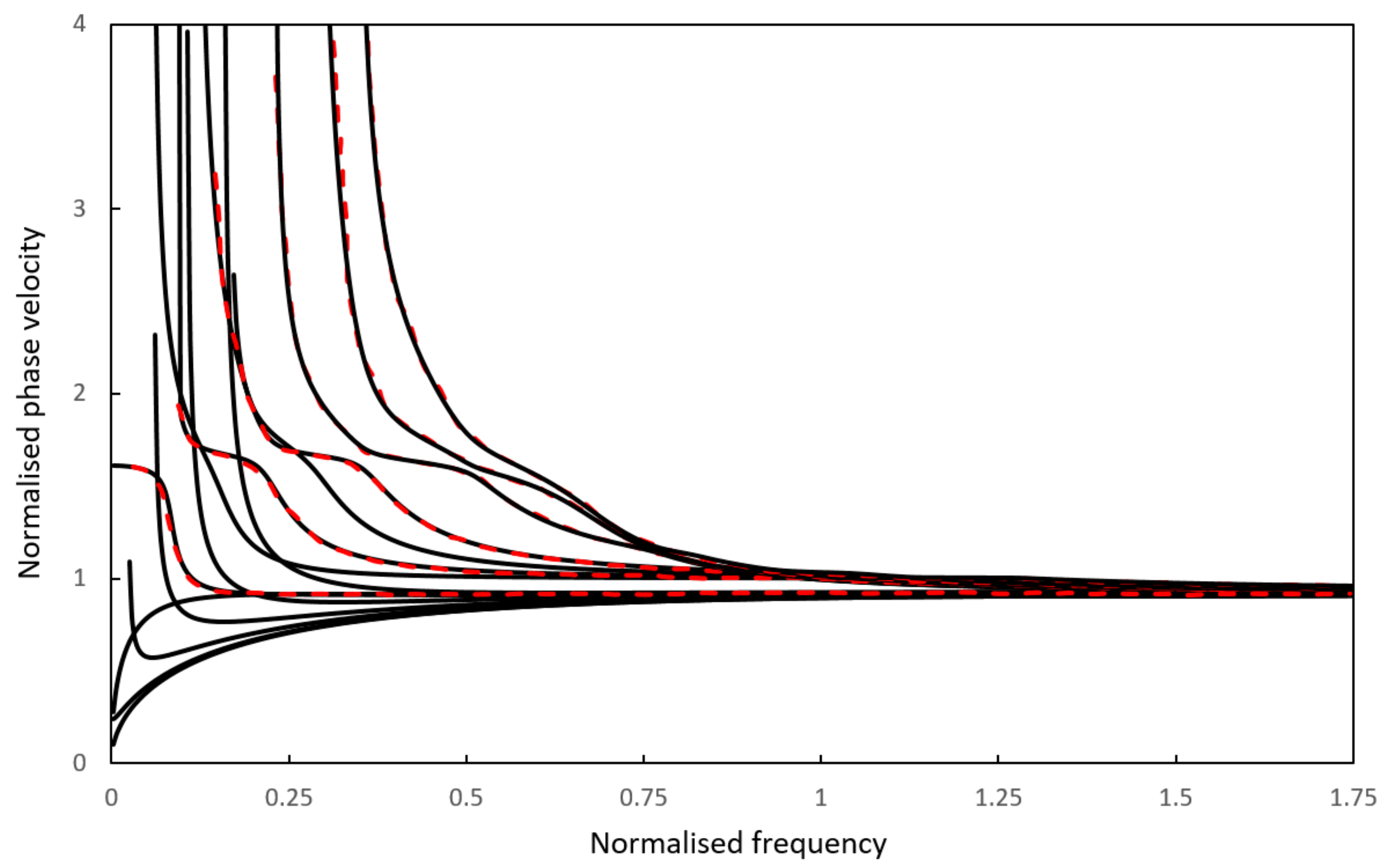
Figure 2.
Dispersion curves for a steel plate with an aspect ratio of 40: (a) phase velocity; (b) group velocity.
Figure 2.
Dispersion curves for a steel plate with an aspect ratio of 40: (a) phase velocity; (b) group velocity.
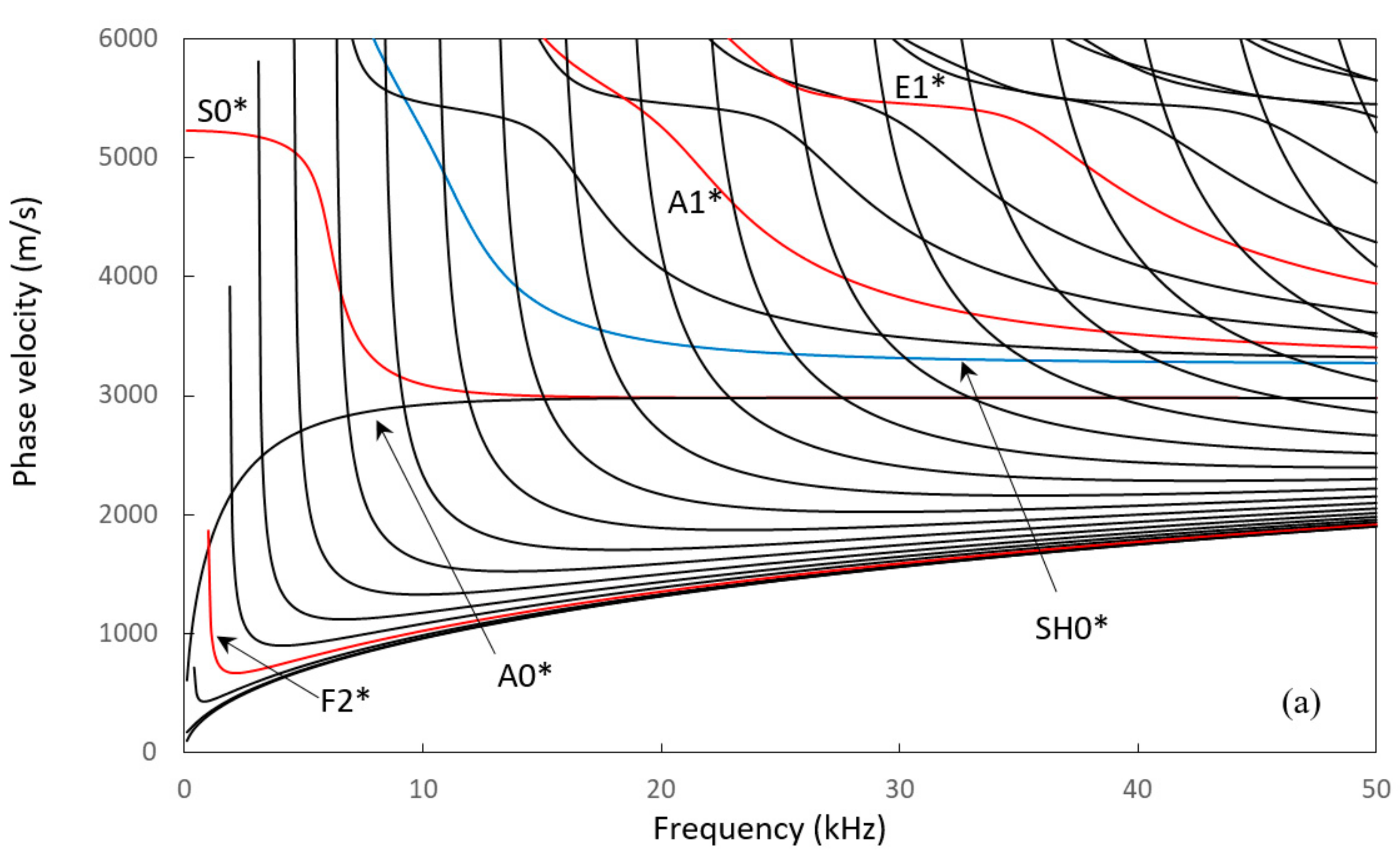

Figure 3.
Dispersion curves for Lamb waves in an infinite plate: (a) phase velocity; (b) group velocity. Red line: 10 mm thickness; black line: 400 mm thickness.
Figure 3.
Dispersion curves for Lamb waves in an infinite plate: (a) phase velocity; (b) group velocity. Red line: 10 mm thickness; black line: 400 mm thickness.

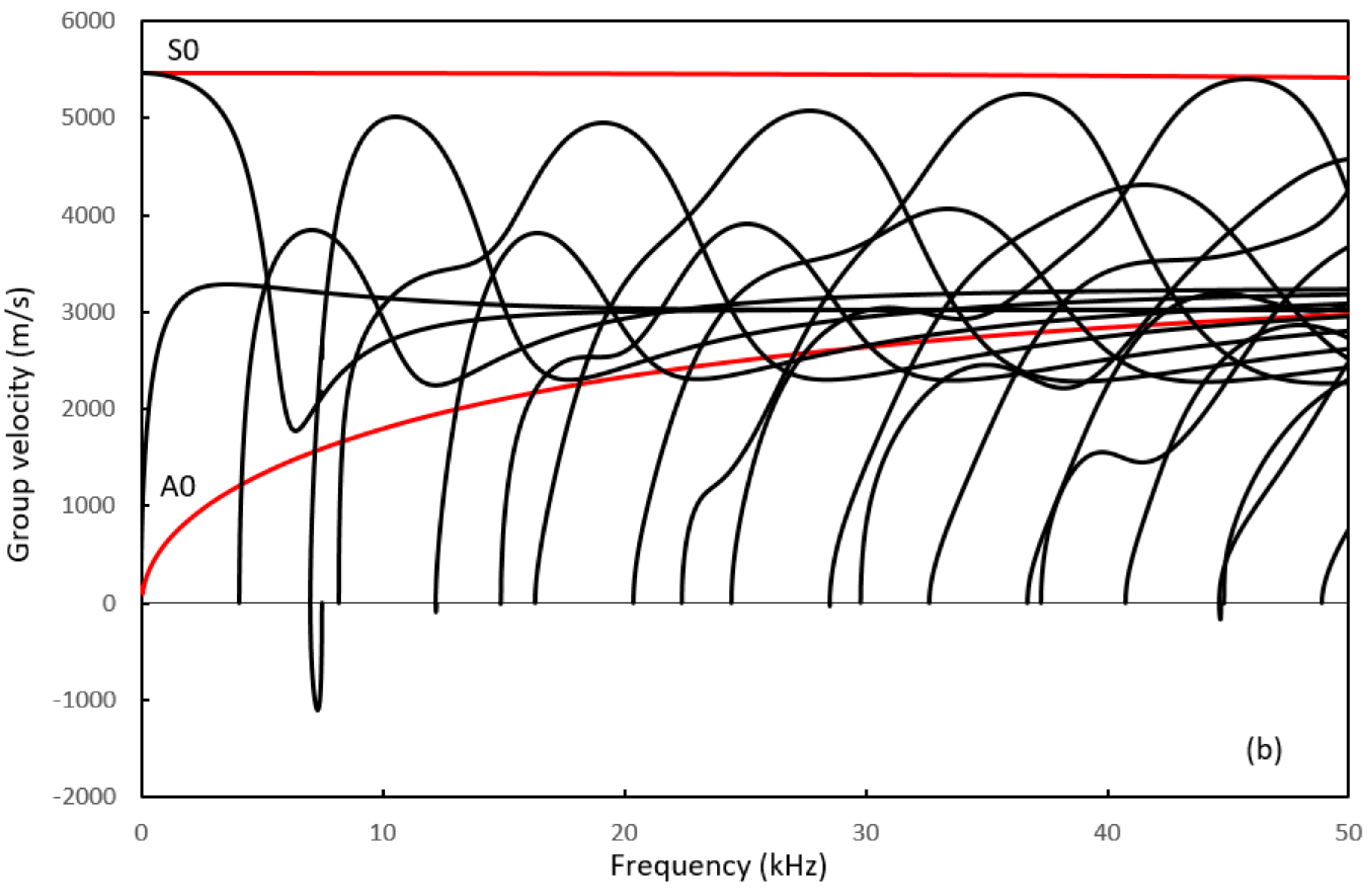
Figure 4.
Point source arrangement to excite a wave mode in the rectangular plate.

Figure 5.
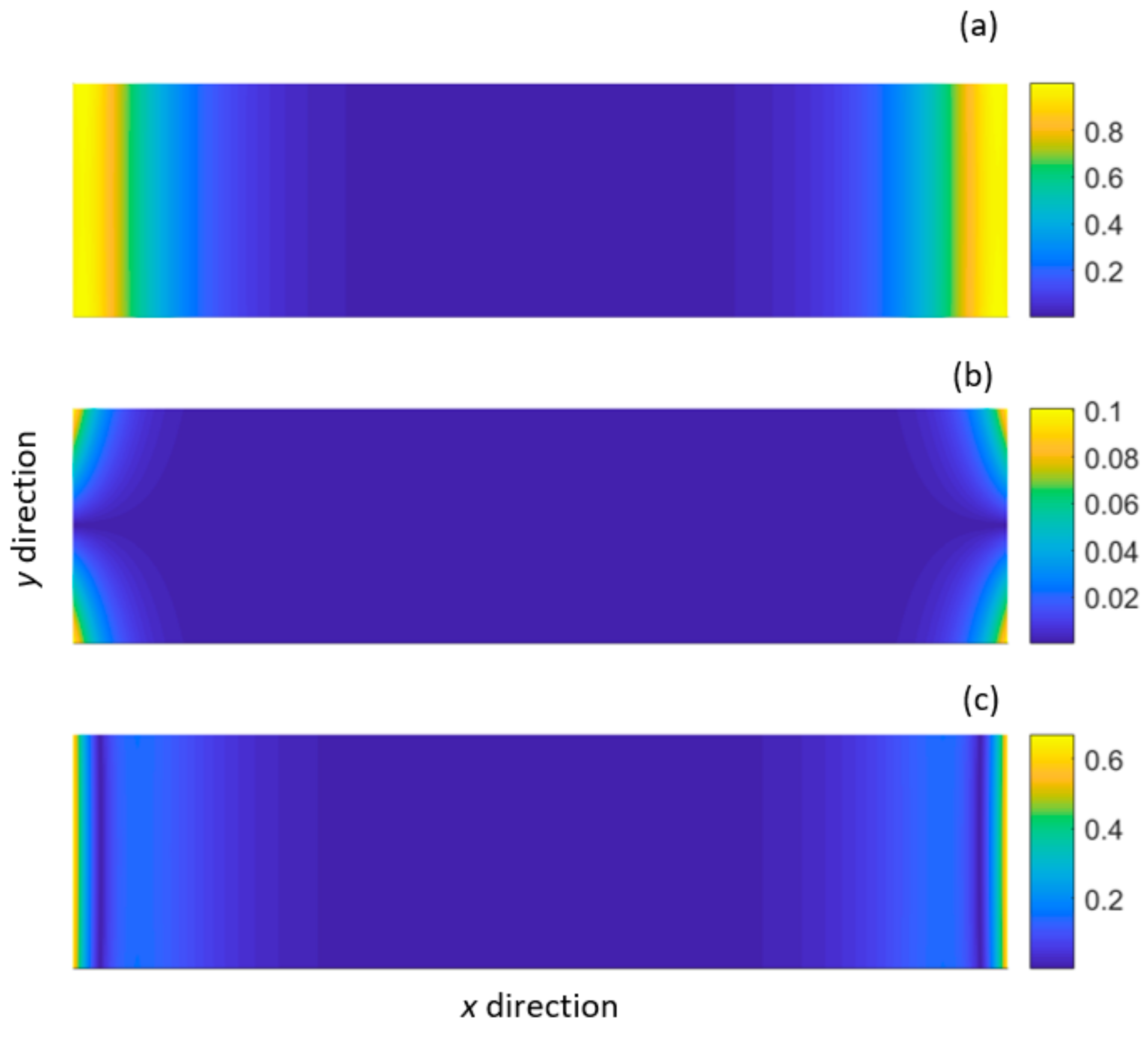
Normalised displacement distribution of the symmetric mode (S0*): (a) shear displacement (x direction); (b) vertical displacement (y direction); (c) extensional displacement (z direction).
Figure 5.
Normalised displacement distribution of the symmetric mode (S0*): (a) shear displacement (x direction); (b) vertical displacement (y direction); (c) extensional displacement (z direction).

Figure 6.
Excitation of Rayleigh mode S0*: (a) shear displacement loading; (b) extensional displacement loading; (c) generated shear displacement distribution (top view); (d) generated shear displacement distribution (transverse view); (e) time domain displacement at receiver position. ![Metals 07 00552 i003]() , 79 point sources;
, 79 point sources; ![Metals 07 00552 i004]() , 39 point sources;
, 39 point sources; ![Metals 07 00552 i005]() , 19 point sources;
, 19 point sources; ![Metals 07 00552 i006]() , 15 point sources.
, 15 point sources.
 , 79 point sources;
  , 39 point sources;
  , 19 point sources;
  , 15 point sources.
Figure 6.
Excitation of Rayleigh mode S0*: (a) shear displacement loading; (b) extensional displacement loading; (c) generated shear displacement distribution (top view); (d) generated shear displacement distribution (transverse view); (e) time domain displacement at receiver position. ![Metals 07 00552 i003]() , 79 point sources;
, 79 point sources; ![Metals 07 00552 i004]() , 39 point sources;
, 39 point sources; ![Metals 07 00552 i005]() , 19 point sources;
, 19 point sources; ![Metals 07 00552 i006]() , 15 point sources.
, 15 point sources.
, 79 point sources; , 39 point sources; , 19 point sources; , 15 point sources.

Figure 7.
Normalised displacement distribution of the shear-horizontal type mode (SH0*): (a) shear displacement (x direction); (b) vertical displacement (y direction); (c) extensional displacement (z direction).
Figure 7.
Normalised displacement distribution of the shear-horizontal type mode (SH0*): (a) shear displacement (x direction); (b) vertical displacement (y direction); (c) extensional displacement (z direction).

Figure 8.
Excitation of shear-type mode SH0*: (a) shear displacement loading; (b) generated shear displacement distribution (top view); (c) time domain displacement at receiver position. ![Metals 07 00552 i007]() , 19 point sources;
, 19 point sources; ![Metals 07 00552 i008]() , 15 point sources;
, 15 point sources; ![Metals 07 00552 i009]() , 9 point sources;
, 9 point sources; ![Metals 07 00552 i010]() , 7 point sources.
, 7 point sources.
 , 19 point sources;
  , 15 point sources;
  , 9 point sources;
  , 7 point sources.
Figure 8.
Excitation of shear-type mode SH0*: (a) shear displacement loading; (b) generated shear displacement distribution (top view); (c) time domain displacement at receiver position. ![Metals 07 00552 i007]() , 19 point sources;
, 19 point sources; ![Metals 07 00552 i008]() , 15 point sources;
, 15 point sources; ![Metals 07 00552 i009]() , 9 point sources;
, 9 point sources; ![Metals 07 00552 i010]() , 7 point sources.
, 7 point sources.
, 19 point sources; , 15 point sources; , 9 point sources; , 7 point sources.
Figure 9.
Excitation of shear-type mode A1*: (a) shear displacement loading; (b) generated shear displacement distribution (top view); (c) time domain displacement at receiver position. ![Metals 07 00552 i011]() , 19 point sources;
, 19 point sources; ![Metals 07 00552 i012]() , 15 point sources;
, 15 point sources; ![Metals 07 00552 i013]() , 9 point sources;
, 9 point sources; ![Metals 07 00552 i014]() , 7 point sources.
, 7 point sources.
 , 19 point sources;
  , 15 point sources;
  , 9 point sources;
  , 7 point sources.
Figure 9.
Excitation of shear-type mode A1*: (a) shear displacement loading; (b) generated shear displacement distribution (top view); (c) time domain displacement at receiver position. ![Metals 07 00552 i011]() , 19 point sources;
, 19 point sources; ![Metals 07 00552 i012]() , 15 point sources;
, 15 point sources; ![Metals 07 00552 i013]() , 9 point sources;
, 9 point sources; ![Metals 07 00552 i014]() , 7 point sources.
, 7 point sources.
, 19 point sources; , 15 point sources; , 9 point sources; , 7 point sources.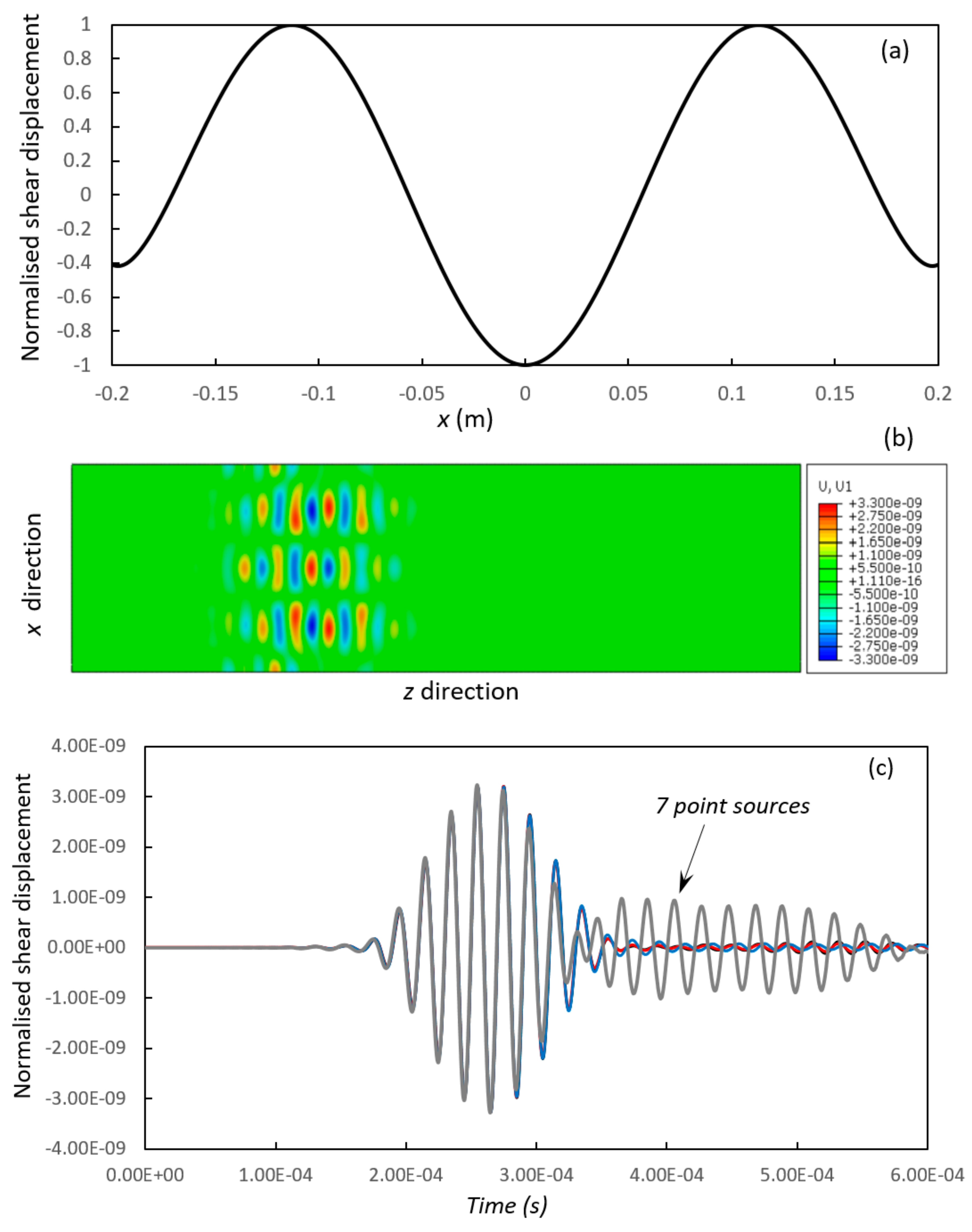
Figure 10.
Normalised displacement distribution of the E1* mode: (a) shear displacement (x direction); (b) vertical displacement (y direction); (c) extensional displacement (z direction).
Figure 10.
Normalised displacement distribution of the E1* mode: (a) shear displacement (x direction); (b) vertical displacement (y direction); (c) extensional displacement (z direction).

Figure 11.
Excitation of extensional type mode E1*: (a) extensional displacement loading; (b) generated extensional displacement distribution (top view); (c) time domain displacement at receiver position. ![Metals 07 00552 i015]() , 19 point sources;
, 19 point sources; ![Metals 07 00552 i016]() , 15 point sources;
, 15 point sources; ![Metals 07 00552 i017]() , 7 point sources;
, 7 point sources; ![Metals 07 00552 i018]() , 3 point sources.
, 3 point sources.
 , 19 point sources;
  , 15 point sources;
  , 7 point sources;
  , 3 point sources.
Figure 11.
Excitation of extensional type mode E1*: (a) extensional displacement loading; (b) generated extensional displacement distribution (top view); (c) time domain displacement at receiver position. ![Metals 07 00552 i015]() , 19 point sources;
, 19 point sources; ![Metals 07 00552 i016]() , 15 point sources;
, 15 point sources; ![Metals 07 00552 i017]() , 7 point sources;
, 7 point sources; ![Metals 07 00552 i018]() , 3 point sources.
, 3 point sources.
, 19 point sources; , 15 point sources; , 7 point sources; , 3 point sources.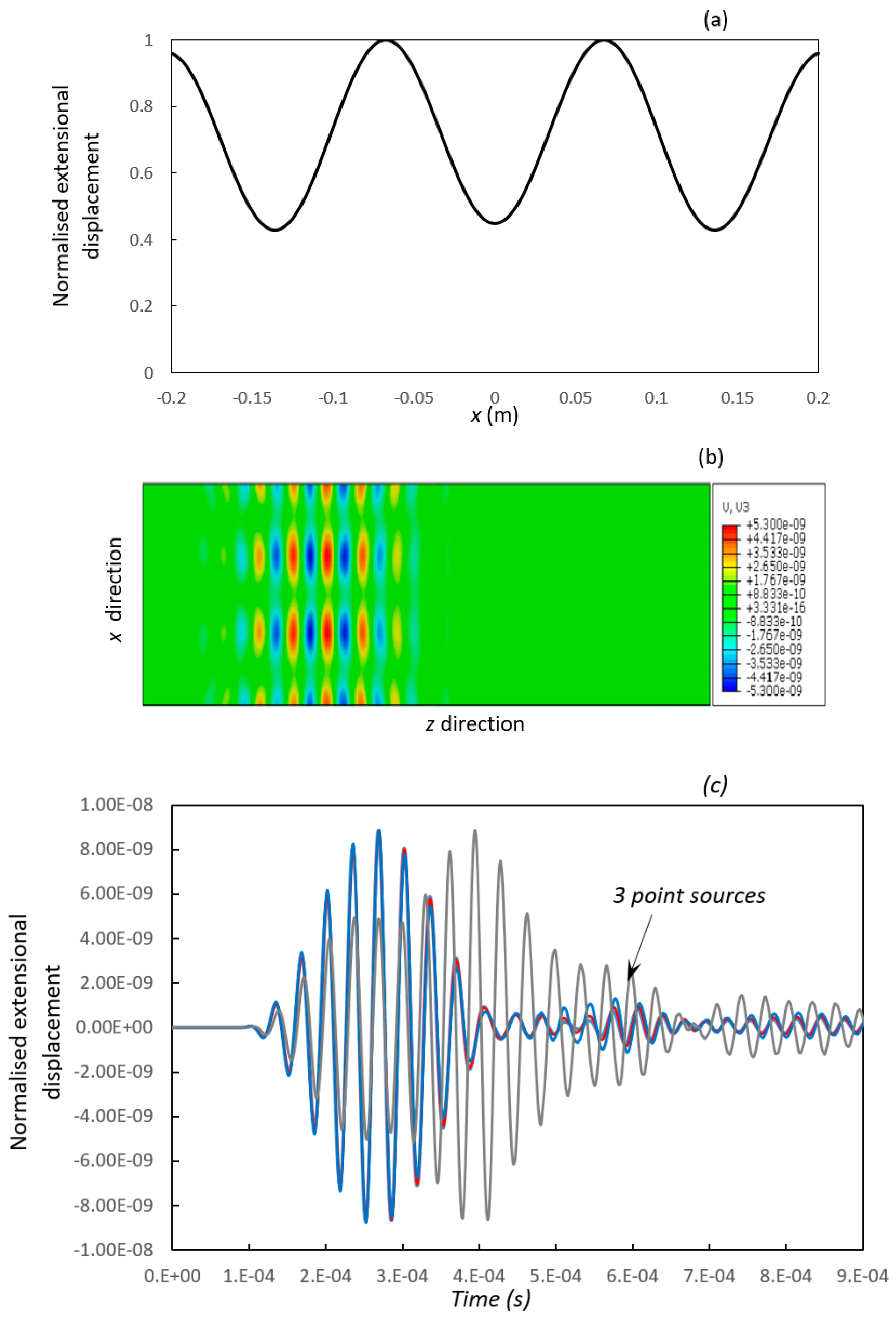
Figure 12.
Normalised displacement distribution of the F2* mode: (a) shear displacement (x direction); (b) vertical displacement (y direction); (c) extensional displacement (z direction).
Figure 12.
Normalised displacement distribution of the F2* mode: (a) shear displacement (x direction); (b) vertical displacement (y direction); (c) extensional displacement (z direction).
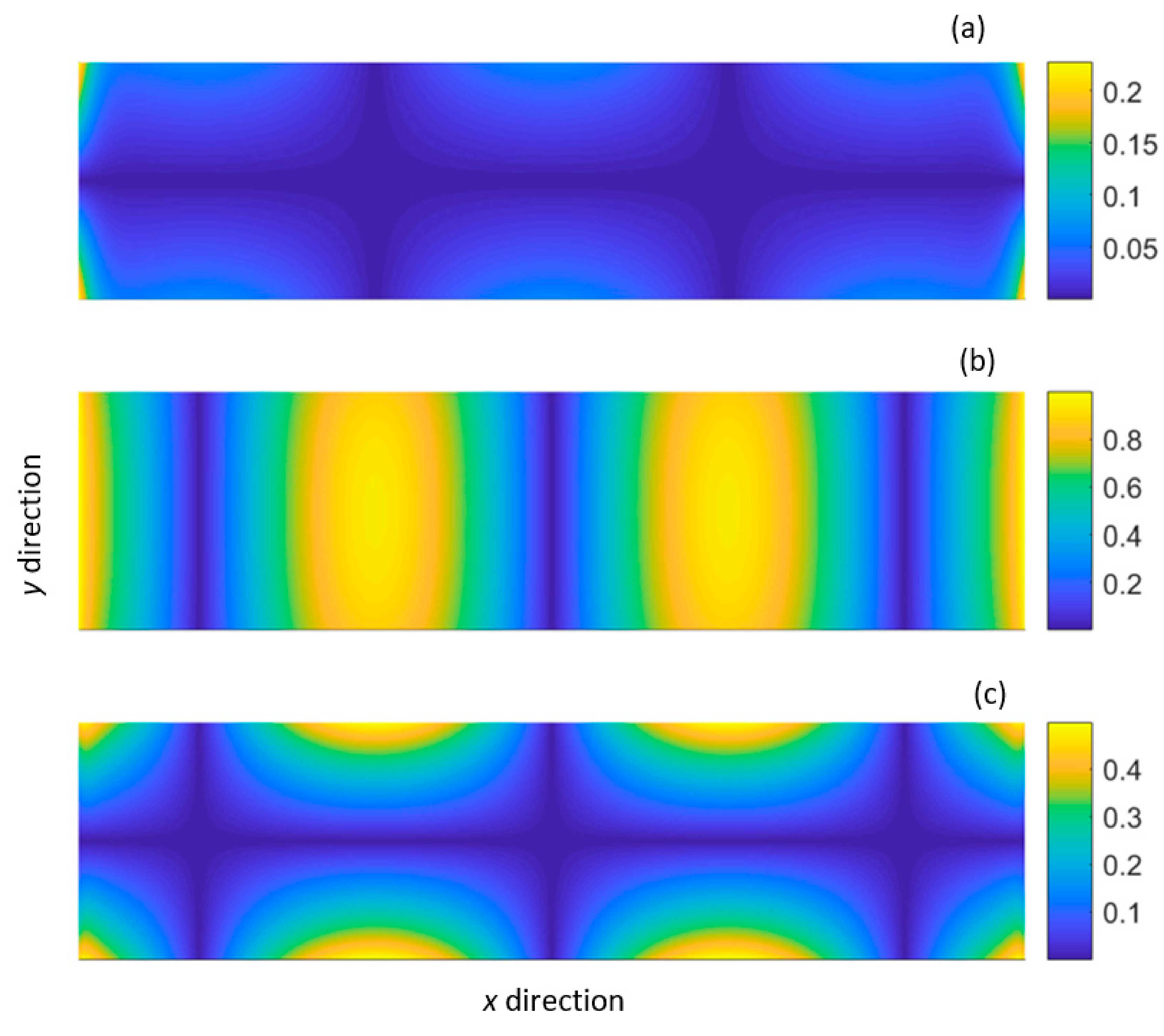
Figure 13.
Excitation of flexural-type mode F2*: (a) vertical displacement loading; (b) generated vertical displacement distribution (top view); (c) time domain displacement at receiver position. ![Metals 07 00552 i019]() , 39 point sources;
, 39 point sources; ![Metals 07 00552 i020]() , 19 point sources;
, 19 point sources; ![Metals 07 00552 i021]() , 15 point sources;
, 15 point sources; ![Metals 07 00552 i022]() , 9 point sources.
, 9 point sources.
 , 39 point sources;
  , 19 point sources;
  , 15 point sources;
  , 9 point sources.
Figure 13.
Excitation of flexural-type mode F2*: (a) vertical displacement loading; (b) generated vertical displacement distribution (top view); (c) time domain displacement at receiver position. ![Metals 07 00552 i019]() , 39 point sources;
, 39 point sources; ![Metals 07 00552 i020]() , 19 point sources;
, 19 point sources; ![Metals 07 00552 i021]() , 15 point sources;
, 15 point sources; ![Metals 07 00552 i022]() , 9 point sources.
, 9 point sources.
, 39 point sources; , 19 point sources; , 15 point sources; , 9 point sources.
© 2017 by the authors. Licensee MDPI, Basel, Switzerland. This article is an open access article distributed under the terms and conditions of the Creative Commons Attribution (CC BY) license (http://creativecommons.org/licenses/by/4.0/).
Share and Cite
MDPI and ACS Style
Duan, W.; Niu, X.; Gan, T.-H.; Kanfoud, J.; Chen, H.-P. A Numerical Study on the Excitation of Guided Waves in Rectangular Plates Using Multiple Point Sources. Metals 2017, 7, 552. https://doi.org/10.3390/met7120552
AMA Style
Duan W, Niu X, Gan T-H, Kanfoud J, Chen H-P. A Numerical Study on the Excitation of Guided Waves in Rectangular Plates Using Multiple Point Sources. Metals. 2017; 7(12):552. https://doi.org/10.3390/met7120552
Chicago/Turabian StyleDuan, Wenbo, Xudong Niu, Tat-Hean Gan, Jamil Kanfoud, and Hua-Peng Chen. 2017. "A Numerical Study on the Excitation of Guided Waves in Rectangular Plates Using Multiple Point Sources" Metals 7, no. 12: 552. https://doi.org/10.3390/met7120552
Note that from the first issue of 2016, this journal uses article numbers instead of page numbers. See further details here.