Modelling of the Superplastic Deformation of the Near-α Titanium Alloy (Ti-2.5Al-1.8Mn) Using Arrhenius-Type Constitutive Model and Artificial Neural Network

Abstract

The paper focuses on developing constitutive models for superplastic deformation behaviour of near-α titanium alloy (Ti-2.5Al-1.8Mn) at elevated temperatures in a range from 840 to 890 °C and in a strain rate range from 2 × 10⁻⁴ to 8 × 10⁻⁴ s⁻¹. Stress–strain experimental tensile tests data were used to develop the mathematical models. Both, hyperbolic sine Arrhenius-type constitutive model and artificial neural-network model were constructed. A comparative study on the competence of the developed models to predict the superplastic deformation behaviour of this alloy was made. The fitting results suggest that the artificial neural-network model has higher accuracy and is more efficient in fitting the superplastic deformation flow behaviour of near-α Titanium alloy (Ti-2.5Al-1.8Mn) at superplastic forming than the Arrhenius-type constitutive model. However, the tested results revealed that the error for the artificial neural-network is higher than the case of Arrhenius-type constitutive model for predicting the unmodelled conditions.

1. Introduction

The flow behaviour of material during hot forming process is usually complicated. The hardening and softening mechanisms both mainly affect the strain rate and temperature [1,2,3]. The understanding of metallic alloys deformation behaviour at elevated temperatures helps to provide information about the metal forming processes. Three main categories of models are utilised to describe the stress flow behavior of metallic alloys: (1) physical based; (2) phenomenological and (3) artificial neural network constitutive models [4,5,6,7,8]. Phenomenological constitutive models are usually used in the simulation of hot forming processes due to their practicability and accuracy. For titanium alloys, the more significant part of literature on the constitutive modelling pays particular attention to α + β type alloys, especially Ti-6Al-4V titanium alloy [8,9,10,11]. The Arrhenius-type constitutive equation (ACE), where the flow stress is expressed by the hyperbolic laws, was first proposed by Jonas et al. [12]. Many studies have used the Arrhenius hyperbolic equation to establish the flow stress of different metallic alloys during deformation at elevated temperatures [6,7].

Recently, artificial neural network (ANN) has provided fundamentally novel and different approaches for materials modelling and processing control from statistical or numerical methods [13]. ANN architecture consists of an input layer, an output layer and one or several hidden layers. Those parts are connected to form a unit called neurons. The input layer is set up to collect data from outside. The output layer sends back the information to the users. The number of hidden layers can vary in function from the amount of data put in the input and output layer. In fact, the hidden layer has the ability of simplifying the complexity of a non-linear problem. The main idea of ANN analysis is to minimise the differences between the known targets of the inputs and the ANN outputs. Therefore, ANN has the capabilities to adjust, memorise and anticipate. Thus, it is thought to be more efficient than regression equations thanks to its extrapolation and interpolation of specific data ranges capabilities. This method provides a new way of using examples of a precise function to find the model constants that will make a specific mapping function with the aim of approximating the function as precisely as possible [14,15]. Furthermore, ANN is especially more suitable in the treatment of non-linear and complicated relationships. It has been increasingly used for modelling the hot deformation behaviour of metallic materials [16,17]. ANN is capable of self and also recognises patterns in a series of input and output values without any prior natural assumptions. ANN does not require any physical knowledge about restoration criteria and deformation. Thus, it is readily suitable to model the hot deformation behaviour of materials in different treatment regimes. ANN offers a good option for modelling because it can keep the data in memory. It can deal with discrete data and adjust the old network to approximate the new experimental data [18]. ANN adjusts itself with the aim of reproducing the function target according to the training sample input. Due to their high ability of parallelism, ANN is truly suitable for estimating the flow stress from experimental data. A back-propagation neural network model was developed to predict the flow stress of Ti-6Al-4V α + β type alloy [19]. The authors of [19] highlighted the possibility of the successful training of the ANN in both β and α + β phase regions. The Arrhenius-type model and the artificial neural network were developed for other Ti40 stable β type titanium alloy [16] and a good agreement between the predicted and the experimental flow stress values was observed in the case of the ANN model.

The purpose of the current study was to suggest a suitable approach for modelling and predicting the deformation behaviour of near-α Ti-2.5Al-1.8Mn alloy, based on superplastic tensile tests data. The Arrhenius constitutive equations were applied to describe the relationship between the flow stress, deformation temperature and constant strain rate at superplastic conditions. The comprehensive model describes the compensation of the strain effect and proposes a relationship between the flow stress, strain rate and temperature of the alloys at elevated temperatures. An ANN model was also developed to predict the flow stress as a function of strain, strain rate and temperature. The validity of the detailed results based on the proposed ACE and ANN model were also compared. The correlation coefficient, the mean absolute relative error and the root mean square error were computed to evaluate the performance of both model types.

2. Materials and Experiments

Conventional sheets of Ti-2.5wt%Al-1.8wt%Mn alloy with a thickness of 1.55 mm were analysed. Superplastic indicators were determined using uniaxial tensile test on a Walter–Bay LFM100 test machine (Walter + Bai AG, Löhningen, Switzerland)) with a DionPro program (Walter + Bai AG, Version. 4.80, Löhningen, Switzerland ) service for the in-situ control traverse motion. The samples were cut parallel to the rolling direction by wire cutting electro-discharge machining process. The gage section size was 6 mm × 1.5 mm, and the gage length was 17 mm. Constant strain rate tests were performed in a temperature range of 840 to 890 °C and constant strain rate values of 2 × 10⁻⁴, 6 × 10⁻⁴ and 8 × 10⁻⁴ s⁻¹. The temperatures and strain rates were within the superplastic deformation strain rate–temperature range according to [20].

3. Test Results

Figure 1 shows the experimental flow stress curves obtained at a constant strain rate values of 2 × 10⁻⁴, 4 × 10⁻⁴ and 8 × 10⁻⁴ s⁻¹ and in a temperature range of 840 to 890 °C. It could be observed that the steady stage begun from the strain value of approximately 0.1. The flow stress values typically increase with increasing strain from 0.1 to 1.3 at all studied conditions. Temperature, strain rate and stress affected the strain hardening behaviour of the studied alloy due to dynamic grain growth phenomenon as described in [20].

The stress–strain data obtained at the various test conditions were used to construct the ACE and ANN models to compare the predictability of both models.

4. Modeling Experiments

4.1. Arrhenius Constitutive Model (ACE)

The influence of strain rate and temperature on deformation behaviour can be expressed via Zener–Holloman parameter (Z) (Equation (1)) and an exponent-type equation (Equation (2)) [21,22,23].

$$Z=\dot{{\epsilon }^{.}}ex{p}^{\frac{Q}{RT}}$$

(1)

$$\dot{{\epsilon }^{.}}=Af\left(\sigma \right)ex{p}^{\left(-\frac{Q}{RT}\right)}$$

(2)

where A is a material constant, $\dot{{\epsilon }^{.}}$ is a strain rate in s⁻¹, T is a temperature in K, and Q is an effective activation energy of deformation in kJ/mol, R is a gas constant = 8.314 J/(mol·K), $f\left(\sigma \right)$ is a function of flow stress, can be expressed as follows:

$$f\left(\sigma \right)=\{\begin{array}{}\left(3\right)& {\sigma }^{n_1},& for\alpha \sigma <0.8\left(4\right)& {exp}^{\left(\beta \sigma \right)},& for\alpha \sigma >1.2\left(5\right)& {\left[\sinh \right(\alpha \sigma \left)\right]}^{n_2},& forvarious\sigma \end{array}$$

where β, $n_1$, n₂ $\mathrm{and}\alpha =$ β/$n_1$ are the material constants. In general, Equation (3) is a power law function, which is appropriable for low stress level $(\alpha \sigma <0.8)$. Equation (4) is an exponential law equation, which is used for high stress level $(\alpha \sigma >1.2)$. Equation (5), a hyperbolic sine law, that typically applies to a wide stress range. Thus, the strain rate can be obtained by the following Equations:

$$\dot{\epsilon }=\{\begin{array}{}\left(6\right)& A_1{\sigma }^{n_1}{exp}^{(-\frac{Q_1}{RT})}-Powerlaw\hfill \left(7\right)& A_2{e}^{\left(\beta \sigma \right)}{exp}^{(-\frac{Q_2}{RT})}-Expontiallaw\hfill \left(8\right)& A_3{\left[\sinh \right(\alpha \sigma \left)\right]}^{n_2}{exp}^{(-\frac{Q_3}{RT})}-Hyperbolicsinelaw\hfill \end{array}$$

4.1.1. Determination of the Arrhenius Constitutive Model Constants

The true stress and true strain data presented in Figure 1 was used to assess the material constants of the constitutive Equations (6)–(8). The true strain of 0.4 (50%) was used as an example to describe the typical procedures of the material constants determination. The following Equations (9) and (10) were obtained by taking the natural logarithm of both sides of Equations (6) and (7):

$$\ln \dot{\epsilon }=\ln A_1+n_1\ln \sigma -\frac{Q_1}{RT}\Rightarrow n_1={\left[\frac{\partial \ln \dot{\epsilon }}{\partial \ln \sigma }\right]}_T$$

(9)

$$\ln \dot{\epsilon }=\ln A_2+\beta \sigma -\frac{Q_2}{RT}\Rightarrow \beta ={\left[\frac{\partial \ln \dot{\epsilon }}{\partial \sigma }\right]}_T$$

(10)

Figure 2 demonstrates the $\ln \dot{\epsilon }-\ln \sigma$ (Figure 2a), $\ln \dot{\epsilon }-\sigma$ (Figure 2b), $\ln \dot{\epsilon }-\ln \sinh \left(\alpha \sigma \right)$ (Figure 2c) and $\ln \sinh \left(\alpha \sigma \right)-\frac{1000}{RT}$ (Figure 2d) linear plots. The slope of plots in Figure 2 varies in limited range. The values of $n_1$, $\beta$ and $Q_{1,2}$ were calculated as the mean values of the slopes of the $\ln \dot{\epsilon }-\ln \sigma$ and $\ln \dot{\epsilon }-\sigma$ plots, respectively (Figure 2a,b).

Equation (11) was obtained by taking the natural logarithm of both sides of Equation (8) to calculate the $Q_3$ and n₂ values:

$$\ln \dot{\epsilon }=\ln A_3+n_2\ln \sinh \left(\alpha \sigma \right)-\frac{Q_3}{RT}$$

(11)

Equations (12) and (13) were obtained by the partial differentiation of Equation (11):

$$n_2={\left[\frac{\partial \ln \dot{\epsilon }}{\partial \ln \left[\sinh \left(\alpha \sigma \right)\right]}\right]}_T$$

(12)

$$Q_3=R\times {\left[\frac{\partial \ln \dot{\epsilon }}{\partial \ln \left[\sinh \left(\alpha \sigma \right)\right]}\right]}_T\times {\left[\frac{\partial \ln \left[\sinh \left(\alpha \sigma \right)\right]}{\partial \left(\frac{1}{T}\right)}\right]}_{\dot{\epsilon }}$$

(13)

Thus, the $n_2$ and $Q_3$ values were achieved from the slope of $\ln \dot{\epsilon }-\ln \sinh \left(\alpha \sigma \right)$ and $\ln \sinh \left(\alpha \sigma \right)-\frac{1000}{RT}$ plotted lines, which are shown in Figure 2c,d.

$Q_1$ and $Q_2$ calculated as same as $Q_3$ as follows:

$$Q_1=R\times {\left[\frac{\partial \ln \dot{\epsilon }}{\partial \ln \sigma }\right]}_T\times {\left[\frac{\partial \ln \sigma }{\partial \left(\frac{1}{T}\right)}\right]}_{\dot{\epsilon }}$$

(14)

$$Q_2=R\times {\left[\frac{\partial \ln \dot{\epsilon }}{\partial \sigma }\right]}_T\times {\left[\frac{\partial \sigma }{\partial \left(\frac{1}{T}\right)}\right]}_{\dot{\epsilon }}$$

(15)

The model parameters at a strain of 0.4 (50%) are collected in

Table 1. The calculated values of A₁, A₂, A₃, n₁, n₂, β, $Q_{1,2,3}$ and α constants of Arrhenius-type constitutive equation (ACE) model.

ln(A1)	n1/m *	Q1 [KJ/mol]	ln(A2)	β [MPa−1]	Q2 [KJ/mol]	α	ln(A3)	n2	Q3 [KJ/mol]
14.6	2.8/0.35	287 ± 12	17.5	0.162	265 ± 10	0.057	21.5	2.166	279 ± 15

* The strain rate sensitivity m-index values were determined as $m=\frac{1}{n_1}$.

.

The relationship between $T, \dot{\epsilon }, \mathrm{and}\sigma$ can be expressed as follows:

$$\dot{\epsilon }=A_3{\left[\sinh \left(\alpha \sigma \right)\right]}^{n_2}ex{p}^{\left(-\frac{Q_3}{RT}\right)}$$

(16)

$$\dot{\epsilon }=2.5\times {10}^9{\left[\sinh \left(0.057\sigma \right)\right]}^{2.166}ex{p}^{\left(-\frac{279\times 1000}{RT}\right)}$$

(17)

Zener–Hollomon parameter Z can be used to describe the flow stress according to the hyperbolic sine law.

$$\sigma =\frac{1}{\alpha }\ln \left\{{\left(\frac{z}{A_3}\right)}^{\frac{1}{n_2}}+{\left[{\left(\frac{z}{A_3}\right)}^{\frac{2}{n_2}}+1\right]}^{\frac{1}{2}}\right\}$$

(18)

where $Z=\dot{\epsilon }ex{p}^{\frac{Q_3}{RT}}$ (Equation (1)).

Finally, the flow stress (σ) versus and the strain rate ($\dot{\epsilon }$) can be described by the follow equation:

$$\sigma =\frac{1}{0.057}\ln \left\{{\left(\frac{\dot{\epsilon }ex{p}^{\frac{279\times {10}^3}{RT}}}{2.5\times {10}^9}\right)}^{\frac{1}{2.166}}+{\left[{\left(\frac{\dot{\epsilon }ex{p}^{\frac{279\times {10}^3}{RT}}}{2.5\times {10}^9}\right)}^{\frac{2}{2.166}}+1\right]}^{\frac{1}{2}}\right\}$$

(19)

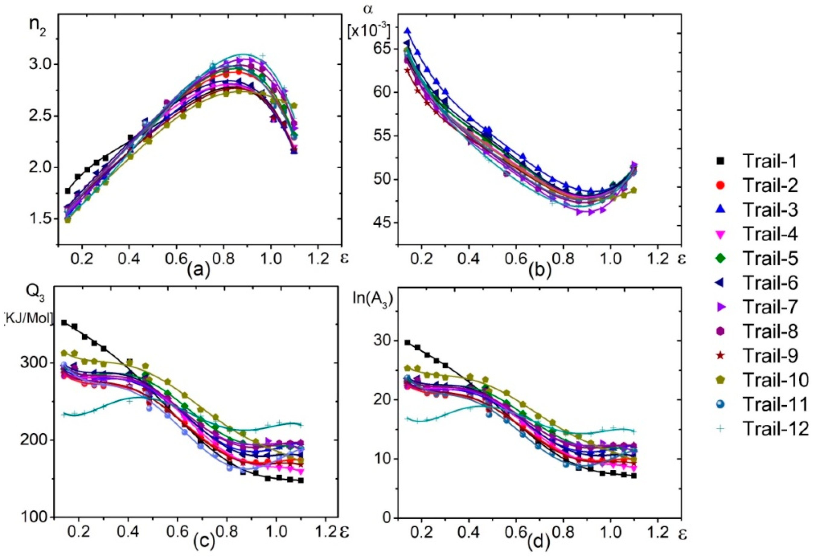
4.1.2. Compensation of Strain Effect

It is known that strain affects the material constants [24,25]. Thus, the strain effect on the material constants should be considered in order to predict the flow stress behavior at deformation. The material constants were determined at different strains within the strain range of 0.1–1.1, as shown in Figure 3. It was considered that the material constants (α, n₂, $Q_3$ and ln(A₃)) exhibit a polynomial relation with the strains according to [24,25,26].

The stress exponent n₂ is typically used to identify the dominant mechanism that controlled the hot deformation process. Thus, the different superplastic deformation mechanisms can be associated with various n₂ values. According to [27,28], grain boundary sliding and dislocation viscous glide mechanism may lead to n values close to 2 and 3 respectively and the mechanisms related to n values in the range of 4 to 6 are associated with dislocation climb. The relationship between n₂ and the strain is consistent with the downward parabola. As shown in Figure 3a, most n₂ values vary from 1.6 to 2.9. Current n₂ values and previously published results of the grain and dislocation structure analysis [20] permits the prediction of the deformation mechanisms and their evolution with increasing strain. The symbioses between the dislocation viscous glide and the grain boundary sliding mechanisms can be used to suggest the deformation controlled mechanism due to n₂ evolution. The grain structure at the start of deformation was partially unrecrystallised. Grain boundary sliding is the main deformation mechanism in the recrystallised volume at the beginning of deformation; thus, the n₂ is closer to 2. The results showed an increase in the value of n₂ to 3 with increasing strain up to 0.8. Grain boundary sliding occurs simultaneously with continuous dynamic recrystallisation in the deformed and the substructured volume with increasing strain. The decrease in the n₂ value at larger strains may be due to the formation of recrystallized grain structure in all tested specimen and the active grain boundary sliding is accommodated by dislocation mechanisms. High dislocation activity in the α-phase was observed at superplastic deformation of the studied alloy at both small strain of 0.7 and large strain of 1.6. Moreover, a fraction of the deformed β-phase is increased with increasing strain according to [20], which suggested that significant deformation of the β-phase occurred due to the dislocation mechanisms.

The material constant α (Figure 3b) presents an overall downward trend with the increase of strain up to 0.8. Constant α decreases in a strain range of 0.8 to 1.0 and insignificantly change in a strain range of 1.0 to 1.1.

The effective activation energy of deformation also suggested the specific deformation mechanisms and the accompanying processes [29]. The effective activation energy ($Q_3$) versus strain (Figure 3c) and ln(A₃) versus strain (Figure 3d) curves exhibit similar behaviour. The effective activation energy $Q_3$ varies in a range from 285 to 180 kJ/mol for the different strain values in a studied temperature range (Figure 3c). The $Q_3$ decreased significantly to a strain value of 0.8 and insignificantly changed. The decrease in $Q_3$ with increasing strain is in agreement with [25,27,28,30]. The decreasing $Q_3$ value clearly indicates a decrease in the amount of stored energy in the material due to deformation [24,29]. Dislocation density at low strains can decrease due to dynamic recovery and recrystallisation at the beginning of the superplastic deformation, which occurred at low stains in the studied alloy according to [20]. The decrease in crystal defects leads to the formation of more equilibrium states and lower $Q_3$.

The activation energies of the grain boundary self-diffusion are 183 kJ·mol⁻¹ in α-Ti and 153 kJ/mol⁻¹ in β-Ti [31]. The intergranular diffusion activation energy is significantly higher for both phases (from 200 to 360 kJ·mol⁻¹ [31]). The constitutive model predicts the effective activation energy of approximately 180 kJ·mol⁻¹ at strains above 0.7. This value is close to the activation energy for the grain boundary self-diffusion in α-Ti. Therefore, the effective activation energy value can be associated with the grain boundary sliding mechanism [32], which is in agreement with the superplastic phenomenon description [33].

Based on the value of R², the fifth order polynomial was found to represent it more accurately. The material parameters α, n₂ and ln(A₃) have good correlation coefficient Equation (20) which means that their behavior can be modeled using the polynomial equations. The coefficients of the polynomial function are presented in

Table 2. The coefficient of the polynomial for α, n₂, A₃ and $Q_3$ and the R² for this coefficient.

Parameter	Y0	B1	B2	B3	B4	B5	R2
$\alpha$	Y10 = 0.077	B11 = −0.135	B12 = 0.363	B13 = −0.55	B14 = 0.387	B15 = −0.096	0.998
$n_2$	Y20 = 1.19	B21 = 2.99	B22 = −1.57	B23 = 0.48	B24 = 2.193	B25 = −2.58	0.995
$\ln (A_3)$	Y30 = 33.17	B31 = −137.03	B32 = 621.85	B33 = −1272	B34 = 1112.9	B35 = −348.2	0.997
$Q$	Y40 = 384.76	B41 = −1269.25	B42 = 5751.1	B43 = −11,719	B44 = 10,220.4	B45 = −3187	0.997

.

$$\{\begin{array}{c}\alpha =Y_{10}+B_{11}{\epsilon }^1+B_{12}{\epsilon }^2+B_{13}{\epsilon }^3+B_{14}{\epsilon }^4+B_{15}{\epsilon }^5\\ n_2=Y_{20}+B_{21}{\epsilon }^1+B_{22}{\epsilon }^2+B_{23}{\epsilon }^3+B_{24}{\epsilon }^4+B_{25}{\epsilon }^5\\ A_3=Y_{30}+B_{31}{\epsilon }^1+B_{32}{\epsilon }^2+B_{33}{\epsilon }^3+B_{34}{\epsilon }^4+B_{35}{\epsilon }^5\\ Q_3=Y_{40}+B_{41}{\epsilon }^1+B_{42}{\epsilon }^2+B_{43}{\epsilon }^3+B_{44}{\epsilon }^4+B_{45}{\epsilon }^5\end{array}$$

(20)

After determining the material constants, the flow stress at an effective strain rate was predicted using Equation (16).

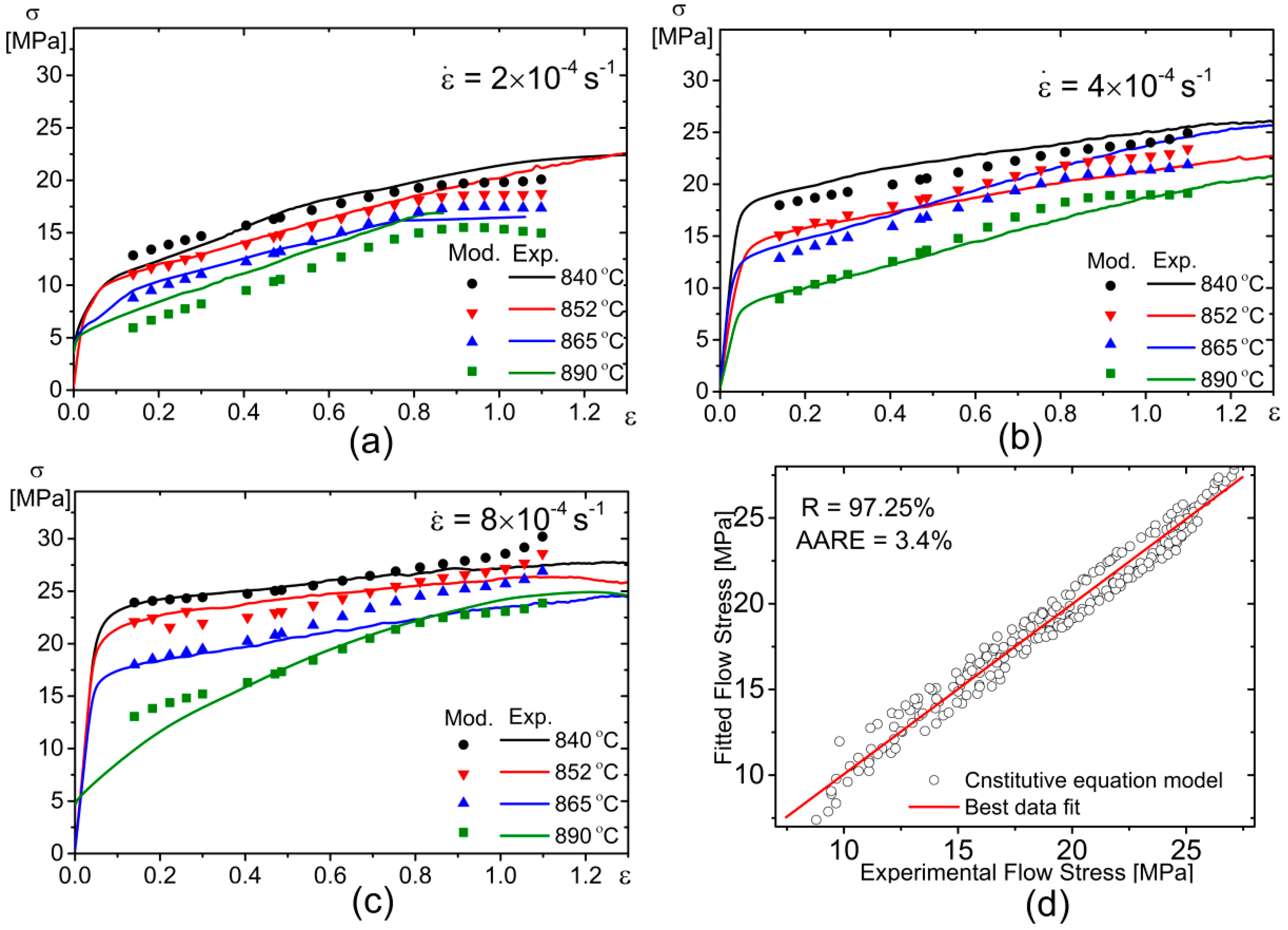
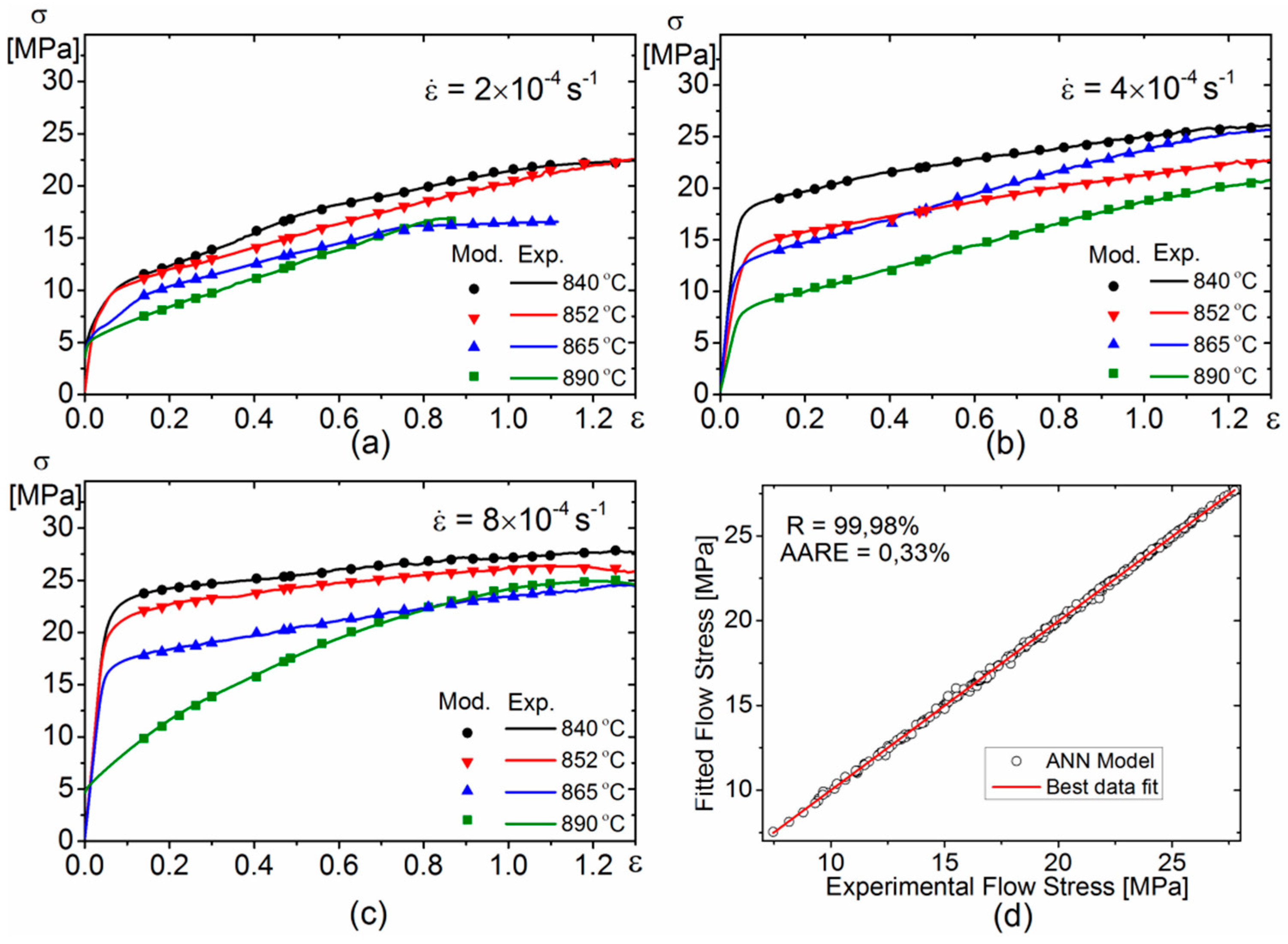
4.1.3. Verification of the Arrhenius Constitutive Equations Model

In order to evaluate the accuracy of the developed ACE equations, a comparison between the fitted and the experimented stress values was performed. The performance of the developed model is evaluated by calculating the correlation coefficient (R) (Equation (21)), average absolute relative error (AARE) (Equation (22)) and the root mean square error (RMSE) (Equation (23)):

$$R=\frac{{\sum }_{i=1}^N\left(E_i-\overline{E}\right)\left(P_i-\overline{P}\right)}{\sqrt{{\sum }_{i=1}^N{\left(E_i-\overline{E}\right)}^2{\sum }_{i=1}^N{\left(P_i-\overline{P}\right)}^2}}$$

(21)

$$AARE=\frac{1}{N}{\displaystyle \sum _{i=1}^N}\left|\frac{E_i-P_i}{E_i}\right|$$

(22)

$$RMSE=\sqrt{\frac{1}{N}{\displaystyle \sum _{i=1}^N}{\left(E_i-P_i\right)}^2}$$

(23)

where E_i is the experimental flow stress, and P_i is the fitted flow stress obtained from the modified constitutive equation. $\overline{E}$ and $\overline{P}$ are the mean values of the experimental and the fitted flow stress values, respectively. N is the total data number that used in current research. R is the statistical index which is typically used to reflect the quality of the correlation between different coefficients. To be useful, the correlation coefficient R requires a significant amount of data. For instance, if the N is too small, the method that provides a relationship between the experimental and the predicted stress may be identified due to the R. In addition, the average absolute relative error (AARE) is an unbiased statistical parameter which may indicate the predictability of an equation and can be calculated term by term.

Figure 4 shows the experimental stress–strain curves with verification of the constitutive equations and the correlation between them in a temperature range of 840–890 °C and a strain rate range of 2 × 10⁻⁴–8 × 10⁻⁴ s⁻¹. It is found that the predicted stresses have a good agreement with the experimental stresses. The values of R, AARE and RMSE are 97.25%, 3.4% and 1.09, respectively. Thus, the results reflect a reasonable predictability of the modified constitutive equation (Figure 4d).

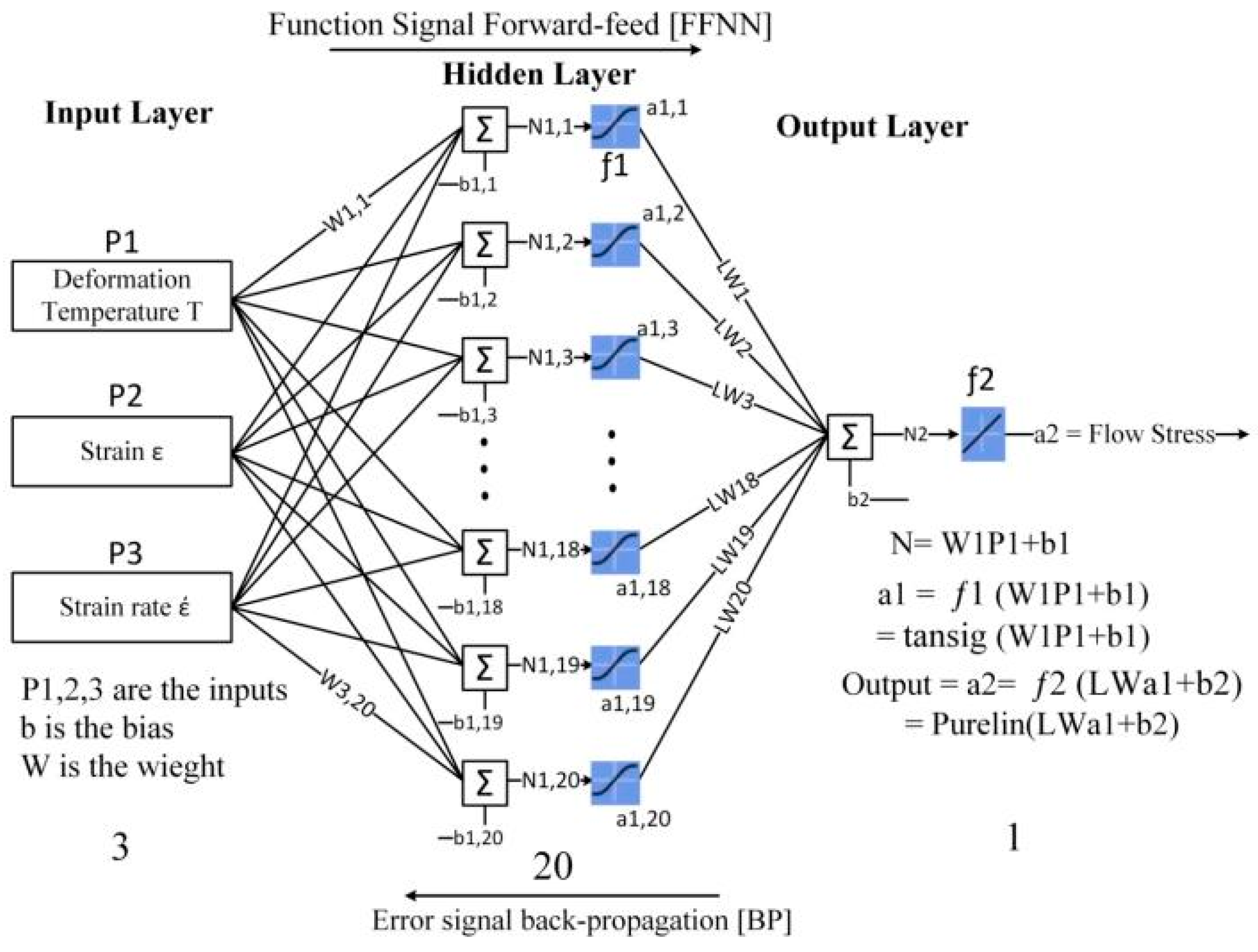
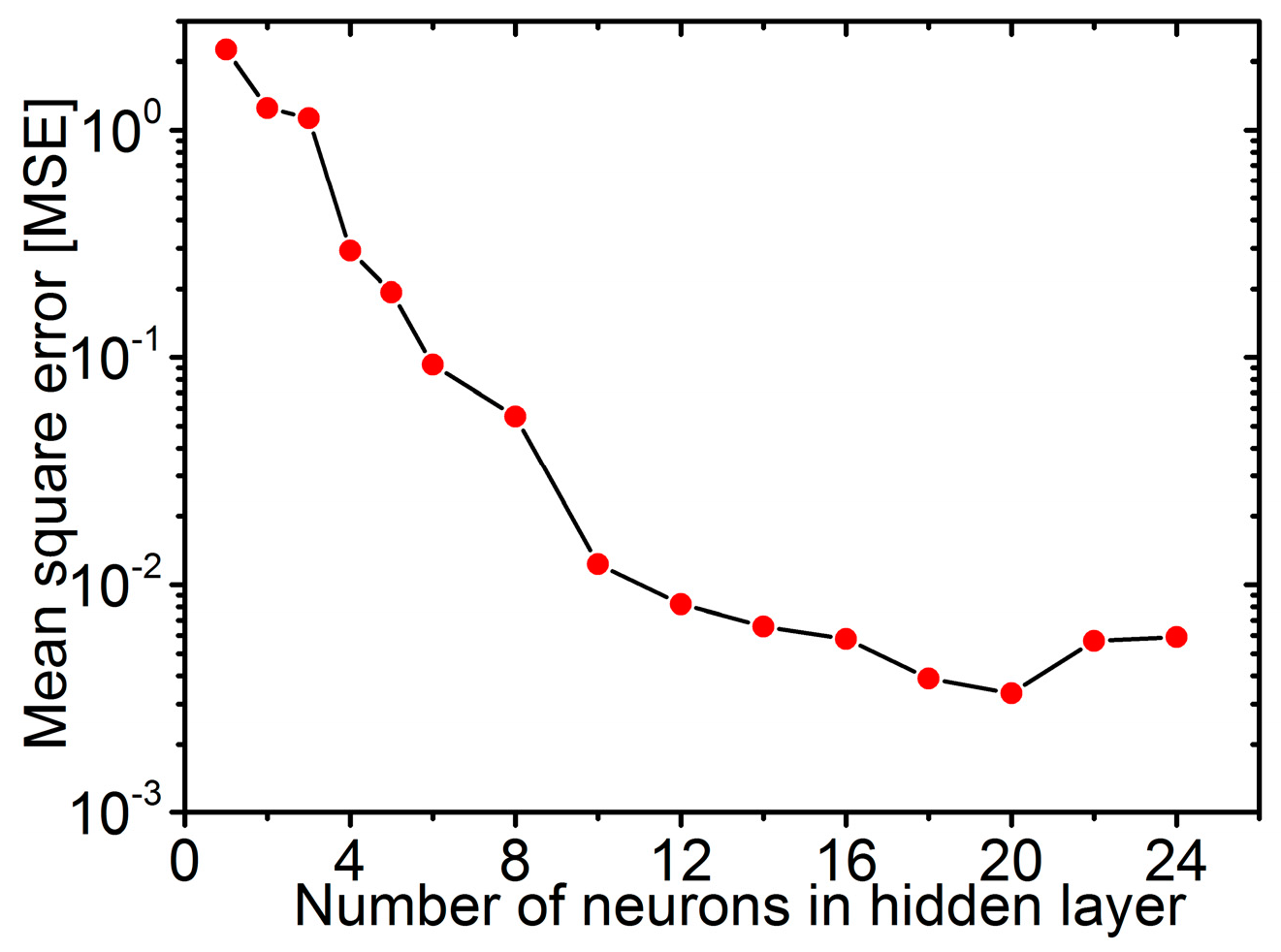
4.2. Artificial Neural Network Analysis

A typical ANN model is generally constructed using various steps, such as: (i) collecting the data; (ii) determining the input/output (target) parameters; (iii) analysing and pre-processing the experimental data; (iv) training the ANN; (v) testing the trained ANN; and, finally, (vi) evaluating the performance of the constructed ANN [34,35,36,37,38,39,40,41,42,43,44]. A popular learning method for algorithms with multilayer observations is back-propagation (BP). It is the standard method for modifying the weights and biases by utilising a gradient descent procedure to reduce the error for a particular training pattern [35]. The ANN with one hidden layer could delineate any function of interest and is truly utilised for many practical problems [38]. In the current work, a typical three-layer back-propagation ANN was consequently used to predict the flow stress behaviour of the studied near-α Titanium alloy Ti-2.5Al-1.8Mn. The strain, strain rate and temperature of deformation were selected as the inputs, and the flow stress values was set as the target in the model. The used ANN architecture is demonstrated in Figure 5.

Both input and target variables were normalised within the range from 0 to 1 before training the supposed model. It was necessary to achieve the network in a right form to be read. As a result, the initial data should be unified to make the ANN training more efficient [37]. The typical method for unifying is expressed as Equation (24):

$$X^{\prime }=\frac{X-0.95X_{\min }}{1.05X_{\max }-0.95X_{\min }}$$

(24)

where X is the initial data value; X_min and X_max are the minimum and maximum values of X, respectively; X′ is the associated data of the corresponding X.

The complex effect of the number of neurons in the hidden layer on the performance of the network is observed similar to [38]. In the case of the simple ANN structure, the trained ANN could not have enough ability to correctly learn the process in order to find the correlation between the input and the target variables. Therefore, it could not converge during training else the trained data may be overfitted. Thus, several network structures with different number of neurons in the hidden layer were studied.

The trial-and-error technique was started with one neuron in the hidden layer and further executed with more neurons. It was required to identify the appropriate number of hidden layers. Figure 6 shows the dependence of the number of neurons in a hidden layer on the network performance. The values of the mean square error (MSE) were used to check the performance of the used ANN. It was noticed that MSE reached the minimum at 20 neurons.

The network’s predictions are refined to approximate the experimental data during training on the basis of the availability of data and the reliability of the target. Training functions, transfer function and training algorithm should be chosen for ANN. In this investigation, the transfer functions that have been used are tan-sigmoid and purelin. The trained network should be tested to show an appropriate reliability and accuracy. Among various possible learning algorithms, the back-propagation algorithm is the most popular utilised for training the ANN [40]. ANN with BP algorithm learns by adjusting the weights, and these adjustments are stored as knowledge.

In this work, the most suitable network was developed to predict the superplastic deformation behaviour of near-α Titanium alloy Ti-2.5Al-1.8Mn alloy. The optimised ANN model consists of three input neurones; a single hidden layer with 20 neurones, one output neurone with transfer functions of ‘tan-sigmoid’ and ‘pure linear’. The feed forward BP algorithm is used to train the ANN. The ANN training parameters are presented in

Table 3. Settings of training parameters for the neural network.

Name of Network Parameters	Contents
Network	Back-Propagation
Training function	TrainLM
Performance function	MSE
Training epoch	8000
Goal	1 × 10−6
Transfer function of hidden layer	Tan-sigmoid
Transfer function of output	Liner (purelin)

. The work was carried out by using the neural network toolbox available in MATLAB 2015b software. The goal of MSE for the training was set as 10⁻⁶. One complete pass through a set of input–output pairs during the training of the network was considered as an epoch [34]. The network was trained to stabilise the error values that was reached after approximately 8000 epochs. It is in agreement with [34].

Figure 7 shows the comparison and the correlation between the fitted and the experimental stresses obtained from the ANN model. As shown, the fitted stresses have an excellent agreement with the experimental stresses at all values of temperature and strain rate. The values of the performance indicators R, AARE and RMSE are 99.98 %, 0.33 % and 0.079 respectively. These values are more accurate than the constitutive equations model. It is in agreement with results observed in other studies [34,35,36,37,38,39,40,41,42,43,44].

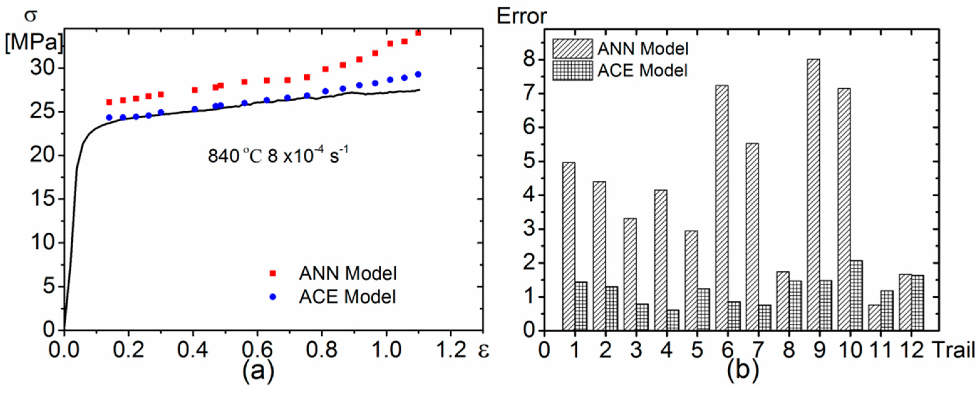
5. Cross-Validation of the Models

In order to find which of the two models (ACE or ANN) predicts the material behaviour better, the cross-validation procedure was utilized. Both models were verified by extracting the stress–strain experimental curves one by one and twelve trial datasets were constructed as listed in

Table 4. The excluded conditions in trial datasets.

Trial Number	Excluded Conditions
	Temperature (°C)	Strain Rate (s−1)
Trial-1	840	2 × 10−4
Trial-2	840	4 × 10−4
Trial-3	840	8 × 10−4
Trial-4	852	2 × 10−4
Trial-5	852	4 × 10−4
Trial-6	852	8 × 10−4
Trial-7	865	2 × 10−4
Trial-8	865	4 × 10−4
Trial-9	865	8 × 10−4
Trial-10	890	2 × 10−4
Trial-11	890	4 × 10−4
Trial-12	890	8 × 10−4

. Both models were subsequently reconstructed for each trial dataset and the predictions made for conditions of excluded stress–strain curve were compared with the experimental data.

Figure 8 shows the material constants versus strain curves calculated for each trial dataset. The material constants nearly exhibit the same behaviour with increasing strain for all trials except for Trails 1 and 12. When the curve at 890 °C and 8 × 10⁻⁴ s⁻¹ was excluded (Trial 12), the effective activation energy at lower strains exhibits lower values compared to the other trials. Conversely, the effective activation energy is higher at lower strains compared to other trials in the case of 840 °C and 2 × 10⁻⁴ s⁻¹ (Trial 1). Trail 1 and Trail 12 are data extremes (Trail 1 is minimum temperature and minimum strain rate; Trail 12 is maximum temperature and maximum strain rate). The extreme points exhibited different behavior compared with the other trails because, the temperature and strain rate were narrow, resulting in simulation error. Simulation error of extremes points can be decreased by increasing the temperature and strain rate ranges. Unfortunately, this observation is cumbersome to analyze because the current alloy exhibits superplasticity in limited temperature–strain rate ranges which were studied.

The error between the experimental and predicted flow stress was calculated as follows (Equation (25)):

$$Error=\frac{1}{{\epsilon }_{\max }}{\displaystyle \underset{0}{\overset{{\epsilon }_{\max }}{\int }}}\left|{\sigma }_{exp.}\left(\epsilon \right)-{\sigma }_{mod.}\left(\epsilon \right)\right| d\epsilon$$

(25)

where ${\sigma }_{exp}\left(\epsilon \right)\mathrm{and}{\sigma }_{mod}\left(\epsilon \right)\mathrm{are}$ the experimental and the predicted flow stresses given as functions of effective strain ($\epsilon$) respectively, ${\epsilon }_{\max }$ is the value of the maximum strain. Figure 9 shows the comparison of the stress–strain curves constructed for Trial-3 (Figure 9a) and the errors between the experimental flow stress and the predicted flow stress of both models (Figure 9b).

It can be clearly seen that even though the ANN model was more accurate in the approximation and the fitting of the initial data than ACE, the ANN error for all trials is higher than that of ACE error (Figure 9). However, after both models have been tested by cross-validation technique, the ACE model exhibits better predictability of the stress values at superplastic deformation compared to the ANN model.

6. Conclusions

Hot tension tests were performed to characterise the flow behaviour of near-α titanium alloy Ti-2.5Al-1.8Mn in a temperature range of 840–890 °C, a strain rate range of 2 × 10⁻⁴–8 × 10⁻⁴ s⁻¹ and a true strain range of 0.1–1.1. The Arrhenius-type constitutive equation (ACE) and the Artificial Neural Network (ANN) were developed to model the superplastic deformation behaviour of the studied alloy.

The following conclusions were drawn from the current results:

(1)

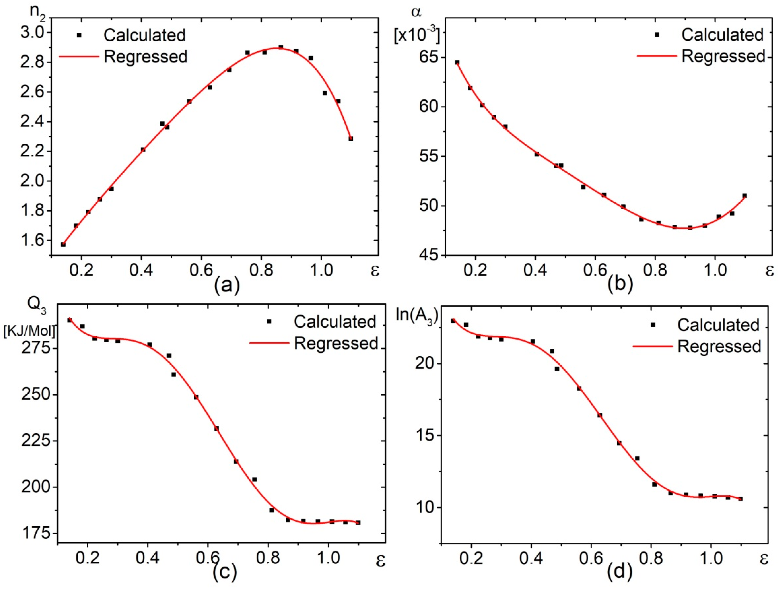
The values of α, n₂, $Q_3$ and A₃ in the Arrhenius-type hyperbolic constitutive equation were found to be the function of strain in the studied strain rate–temperature–strain range. The material constant versus strain dependence suggested that, the symbiosis between the dislocation viscous glide and the grain boundary sliding are the deformation mechanisms.

(2)

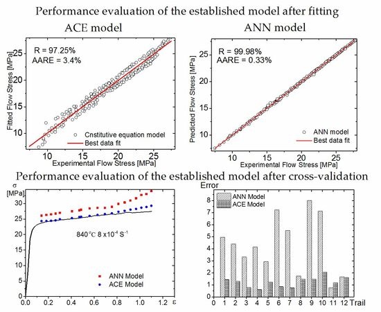
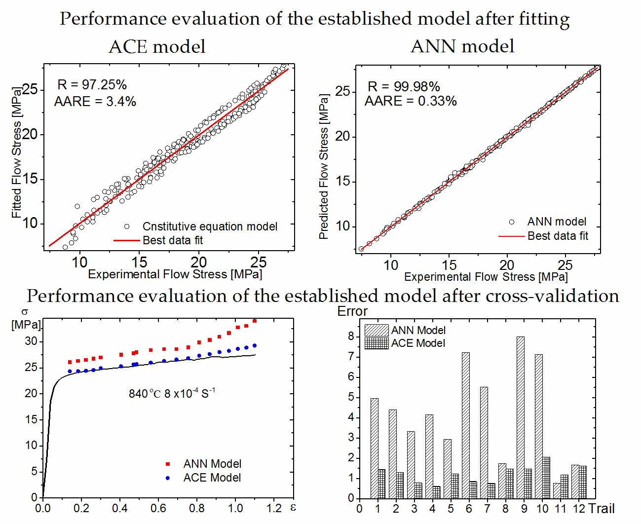
The correlation coefficient (R), the mean absolute relative error (AARE) and the root mean square error (RMSE) obtained from the developed ACE and ANN are 95.25%, 5.2% and 1.09, respectively for the constitutive equations. In the case of ANN, the value of R, AARE and RMSE are 99.97%, 0.32% and 0.079 respectively. The ANN model exhibits higher accuracy and much better efficiency in approximating the hot deformation behaviour than the ACE at the points used for training in ANN.

(3)

Both models were verified by extracting the stress–strain experimental curves one by one, and comparing their predictability following the cross-validation approach. The ACE model exhibits better predictability of the superplastic deformation behavior as compared to the ANN model. An important outcome of this analysis is that, despite the rising popularity of the artificial neural networks, one should exercise caution when using them for predicting mechanical behaviour of materials. Cross-validation should be mandatory for such kind of ANN usage. In some cases, as shown in this work, the verification technique demonstrated that the classical approach based on the constitutive equations of Arrhenius type is more effective and reliable than the artificial neural networks.

References

- Franciosi, P.; Berbenni, S. Heterogeneous crystal and poly-crystal plasticity modeling from a transformation field analysis within a regularized Schmid law. J. Mech. Phys. Solids 2007, 55, 2265–2299. [Google Scholar] [CrossRef]
- Sommitsch, C.; Sievert, R.; Wlanis, T.; Günther, B.; Wieser, V. Modelling of creep-fatigue in containers during aluminium and copper extrusion. Comput. Mater. Sci. 2007, 39, 55–64. [Google Scholar] [CrossRef]
- Dan, W.J.; Zhang, W.G.; Li, S.H.; Lin, Z.Q. A model for strain-induced martensitic transformation of TRIP steel with strain rate. Comput. Mater. Sci. 2007, 40, 101–107. [Google Scholar] [CrossRef]
- Haghdadi, N.; Zarei-Hanzaki, A.; Abedi, H.R. The flow behavior modeling of cast A356 aluminum alloy at elevated temperatures considering the effect of strain. Mater. Sci. Eng. A 2012, 535, 252–257. [Google Scholar] [CrossRef]
- Marandi, A.; Zarei-Hanzaki, A.; Haghdadi, N.; Eskandari, M. The prediction of hot deformation behavior in Fe-21Mn-2.5Si-1.5Al transformation-twinning induced plasticity steel. Mater. Sci. Eng. A 2012, 554, 72–78. [Google Scholar] [CrossRef]
- Zhang, H.; Wen, W.; Cui, H.; Xu, Y. A modified Zerilli-Armstrong model for alloy IC10 over a wide range of temperatures and strain rates. Mater. Sci. Eng. A 2009, 527, 328–333. [Google Scholar] [CrossRef]
- Voyiadjis, G.Z.; Almasri, A.H. A physically based constitutive model for fcc metals with applications to dynamic hardness. Mech. Mater. 2008, 40, 549–563. [Google Scholar] [CrossRef]
- Lin, Y.C.; Chen, X.-M. A critical review of experimental results and constitutive descriptions for metals and alloys in hot working. Mater. Des. 2011, 32, 1733–1759. [Google Scholar] [CrossRef]
- Vanderhasten, M.; Rabet, L.; Verlinden, B. Ti–6Al–4V: Deformation map and modelisation of tensile behavior. Mater. Des. 2008, 29, 1090–1098. [Google Scholar] [CrossRef]
- Cai, J.; Li, F.; Liu, T.; Chen, B.; He, M. Constitutive equations for elevated temperature flow stress of Ti-6Al-4V alloy considering the effect of strain. Mater. Des. 2011, 32, 1144–1151. [Google Scholar] [CrossRef]
- Shafaat, M.A.; Omidvar, H.; Fallah, B. Prediction of hot compression flow curves of Ti-6Al-4V alloy in α+β phase region. Mater. Des. 2011, 32, 4689–4695. [Google Scholar] [CrossRef]
- Jonas, J.J.; Sellars, C.M.; Tegart, W.J.M. Strength and structure under hot-working conditions. Metall. Rev. 1969, 14, 1–24. [Google Scholar] [CrossRef]
- Bahrami, A.; Anijdan, S.H.M.; Hosseini, H.R.M.; Shafyei, A.; Narimani, R. Effective parameters modeling in compression of an austenitic stainless steel using artificial neural network. Comput. Mater. Sci. 2005, 34, 335–341. [Google Scholar] [CrossRef]
- Guo, Z.; Malinov, S.; Sha, W. Modelling beta transus temperature of titanium alloys using artificial neural network. Comput. Mater. Sci. 2005, 32, 1–12. [Google Scholar] [CrossRef]
- Malinov, S.; Sha, W. Application of artificial neural networks for modelling correlations in titanium alloys. Mater. Sci. Eng. A 2004, 365, 202–211. [Google Scholar] [CrossRef]
- Sun, Y.; Zeng, W.D.; Zhao, Y.Q.; Zhang, X.M.; Shu, Y.; Zhou, Y.G. Modeling constitutive relationship of Ti40 alloy using artificial neural network. Mater. Des. 2011, 32, 1537–1541. [Google Scholar] [CrossRef]
- Mandal, S.; Sivaprasad, P.V.; Venugopal, S. Capability of a Feed-Forward Artificial Neural Network to Predict the Constitutive Flow Behavior of As Cast 304 Stainless Steel Under Hot Deformation. J. Eng. Mater. Technol. 2006, 129, 242–247. [Google Scholar] [CrossRef]
- Qin, Y.J.; Pan, Q.L.; He, Y.B.; Li, W.B.; Liu, X.Y.; Fan, X. Artificial Neural Network Modeling to Evaluate and Predict the Deformation Behavior of ZK60 Magnesium Alloy During Hot Compression. Mater. Manuf. Process. 2010, 25, 539–545. [Google Scholar] [CrossRef]
- Reddy, N.S.; Lee, Y.H.; Park, C.H.; Lee, C.S. Prediction of flow stress in Ti-6Al-4V alloy with an equiaxed α+β microstructure by artificial neural networks. Mater. Sci. Eng. A 2008, 492, 276–282. [Google Scholar] [CrossRef]
- Mikhaylovskaya, A.V.; Mosleh, A.O.; Kotov, A.D.; Kwame, J.S.; Pourcelot, T.; Golovin, I.S.; Portnoy, V.K. Superplastic deformation behaviour and microstructure evolution of near-α Ti-Al-Mn alloy. Mater. Sci. Eng. A 2017, 708, 469–477. [Google Scholar] [CrossRef]
- Samantaray, D.; Mandal, S.; Bhaduri, A.K.; Sivaprasad, P.V. An overview on constitutive modelling to predict elevated temperature flow behaviour of fast reactor structural materials. Trans. Indian Inst. Met. 2010, 63, 823–831. [Google Scholar] [CrossRef]
- Zener, C.; Hollomon, J.H. Effect of Strain Rate Upon Plastic Flow of Steel. J. Appl. Phys. 1944, 15, 22–32. [Google Scholar] [CrossRef]
- Sellars, C.M.; McTegart, W.J. On the mechanism of hot deformation. Acta Metall. 1966, 14, 1136–1138. [Google Scholar] [CrossRef]
- Rao, K.P.; Hawbolt, E.B. Development of Constitutive Relationships Using Compression Testing of a Medium Carbon Steel. J. Eng. Mater. Technol. 1992, 114, 116–123. [Google Scholar] [CrossRef]
- Mandal, S.; Rakesh, V.; Sivaprasad, P.V.; Venugopal, S.; Kasiviswanathan, K.V. Constitutive equations to predict high temperature flow stress in a Ti-modified austenitic stainless steel. Mater. Sci. Eng. A 2009, 500, 114–121. [Google Scholar] [CrossRef]
- Lin, Y.C.; Chen, M.-S.; Zhong, J. Constitutive modeling for elevated temperature flow behavior of 42CrMo steel. Comput. Mater. Sci. 2008, 42, 470–477. [Google Scholar] [CrossRef]
- Mahmudi, R.; Rezaee-Bazzaz, A.; Banaie-Fard, H.R. Investigation of stress exponent in the room-temperature creep of Sn-40Pb-2.5Sb solder alloy. J. Alloys Compd. 2007, 429, 192–197. [Google Scholar] [CrossRef]
- Langdon, T.G. Identifiying creep mechanisms at low stresses. Mater. Sci. Eng. A 2000, 283, 266–273. [Google Scholar] [CrossRef]
- Yang, X.; Guo, H.; Liang, H.; Yao, Z.; Yuan, S. Flow Behavior and Constitutive Equation of Ti-6.5Al-2Sn-4Zr-4Mo-1W-0.2Si Titanium Alloy. J. Mater. Eng. Perform. 2016, 25, 1347–1359. [Google Scholar] [CrossRef]
- Pu, Z.J.; Wu, K.H.; Shi, J.; Zou, D. Development of constitutive relationships for the hot deformation of boron microalloying TiAlCrV alloys. Mater. Sci. Eng. A 1995, 192–193, 780–787. [Google Scholar] [CrossRef]
- Weiss, I.; Semiatin, S.L. Thermomechanical processing of alpha titanium alloys—An overview. Mater. Sci. Eng. A 1999, 263, 243–256. [Google Scholar] [CrossRef]
- Frost, H.J.; Ashby, M.F. Deformation Mechanism Maps: The Plasticity and Creep of Metals and Ceramics, 1st ed.; Pergamon Press: New York, NY, USA, 1982; p. 166. ISBN 0080293379. [Google Scholar]
- Nieh, T.G.; Wadsworth, J.; Sherby, O.D. Superplasticity in Metals and Ceramics, 1st ed.; Cambridge University Press: Cambridge, UK, 1997; p. 288. ISBN 100521561051. [Google Scholar]
- Zhao, J.; Ding, H.; Zhao, W.; Huang, M.; Wei, D.; Jiang, Z. Modelling of the hot deformation behaviour of a titanium alloy using constitutive equations and artificial neural network. Comput. Mater. Sci. 2014, 92, 47–56. [Google Scholar] [CrossRef]
- Genel, K.; Kurnaz, S.C.; Durman, M. Modeling of tribological properties of alumina fiber reinforced zinc–aluminum composites using artificial neural network. Mater. Sci. Eng. A 2003, 363, 203–210. [Google Scholar] [CrossRef]
- Hornik, K.; Stinchcombe, M.; White, H. Multilayer feedforward networks are universal approximators. Neural Netw. 1989, 2, 359–366. [Google Scholar] [CrossRef]
- Wu, S.W.; Zhou, X.G.; Cao, G.M.; Liu, Z.Y.; Wang, G.D. The improvement on constitutive modeling of Nb-Ti micro alloyed steel by using intelligent algorithms. Mater. Des. 2017, 116, 676–685. [Google Scholar] [CrossRef]
- Guo, L.F.; Li, B.C.; Xue, Y.; Zhang, Z.M. Constitutive Relationship Model of Al-W Alloy Using Artificial Neural Network. Adv. Mater. Res. 2014, 1004–1005, 1120–1124. [Google Scholar] [CrossRef]
- Ji, G.; Li, F.; Li, Q.; Li, H.; Li, Z. A comparative study on Arrhenius-type constitutive model and artificial neural network model to predict high-temperature deformation behaviour in Aermet100 steel. Mater. Sci. Eng. A 2011, 528, 4774–4782. [Google Scholar] [CrossRef]
- Sun, Y.; Zeng, W.D.; Zhao, Y.Q.; Qi, Y.L.; Ma, X.; Han, Y.F. Development of constitutive relationship model of Ti600 alloy using artificial neural network. Comput. Mater. Sci. 2010, 48, 686–691. [Google Scholar] [CrossRef]
- Peng, W.; Zeng, W.; Wang, Q.; Yu, H. Comparative study on constitutive relationship of as-cast Ti60 titanium alloy during hot deformation based on Arrhenius-type and artificial neural network models. Mater. Des. 2013, 51, 95–104. [Google Scholar] [CrossRef]
- Li, H.Y.; Wei, D.D.; Li, Y.H.; Wang, X.F. Application of artificial neural network and constitutive equations to describe the hot compressive behavior of 28CrMnMoV steel. Mater. Des. 2012, 35, 557–562. [Google Scholar] [CrossRef]
- Haghdadi, N.; Zarei-Hanzaki, A.; Khalesian, A.R.; Abedi, H.R. Artificial neural network modeling to predict the hot deformation behavior of an A356 aluminum alloy. Mater. Des. 2013, 49, 386–391. [Google Scholar] [CrossRef]
- Guo, L.; Li, B.; Zhang, Z. Constitutive relationship model of TC21 alloy based on artificial neural network. Trans. Nonferr. Met. Soc. China 2013, 23, 1761–1765. [Google Scholar] [CrossRef]