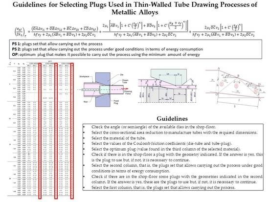
Guidelines for Selecting Plugs Used in Thin-Walled Tube Drawing Processes of Metallic Alloys


Department of Manufacturing Engineering, Industrial Engineering School, Universidad Nacional de Educación a Distancia (UNED), St/Juan del Rosal 12, E28040 Madrid, Spain
*
Author to whom correspondence should be addressed.
Metals 2017, 7(12), 572; https://doi.org/10.3390/met7120572
Submission received: 18 November 2017
/
Revised: 11 December 2017
/
Accepted: 13 December 2017
/
Published: 18 December 2017
(This article belongs to the Special Issue Metallic Materials and Manufacturing)
Abstract
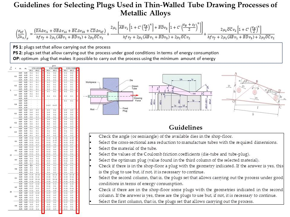
:In this paper, some practical guidelines to select the plug or set of plugs more adequate to carry out drawing processes of thin-walled tubes carried out with fixed conical inner plug are presented. For this purpose, the most relevant input parameters have been considered in this study: the tube material, the most important geometrical parameters of the process (die semiangle, , and cross-sectional area reduction, ) and the friction conditions (Coulomb friction coefficients, , between the die and the tube outer surface, and , between the plug and the tube inner surface). Three work-hardening materials are analyzed: the annealed copper UNS C11000, the aluminum UNS A91100, and the stainless steel UNS S34000. The analysis is realized by means of the upper bound method (UBM), modelling the plastic deformation zone by triangular rigid zones (TRZ), under the validated assumption that the process occurs under plane strain conditions. The obtained results allow establishing, for each material, a group of geometrical parameters, friction conditions, a set of plugs that make possible to carry out the process under good conditions, and the optimum plug to carry out the process using the minimum amount of energy. The proposed model is validated by means of an own finite element analysis (FEA) carried out under different conditions and, in addition, by other finite element method (FEM) simulations and real experiments taken from other researchers found in the literature (called literature simulations and literature experimental results, respectively). As a main conclusion, it is possible to affirm that the plug that allows carrying out the process with minimum quantity of energy is cylindrical in most cases.
1. Introduction
Axisymmetric drawing is extensively used in the industry for manufacturing different kind of components, mainly in the shape of bars/rods, wires, and tubes. In the last decades, a lot of research has been developed in order to analyze this group of metal forming processes and particularly their main characteristics and interrelations between the variables involved. Thus, Celentano et al. [1] have analyzed the mechanical behaviour of steel rods during multiple-step wire cold-drawing processes by numerical and experimental techniques, assessing the influence of the number of wire reductions and the presence of back tension on the material response during the process. The influence of back tension was also studied by the authors in their previous work [2]. Another study [3] was focused on obtaining the drawing stresses required to carry out the process, modelling wire and plate drawing operations by an analytical method such as the slab method (SM) and a numerical one such as the finite element method (FEM). The results were also compared with results found in the literature [4,5,6,7,8,9,10,11,12,13,14,15,16,17,18,19,20,21,22,23,24,25,26,27,28,29,30,31], particularly with Wistreich’s experimental solutions in wire drawing and with Green and Hill and the upper bound technique in plate drawing. The work of Vega et al. [4] investigated the effect of the process variables such as semi-die angle and reduction in area, and the coefficient of friction on the drawing forces of copper wires, paying attention to the die design in order to obtain the best quality of wire. Some other studies have focused on analyzing the influence of geometrical conditions on the appearance of internal defects such as the well-known central burst or chevron crack [5]. In the work of McAllen and Phelan [6], they presented a modified damage model that was implemented into a finite element model using a Fortran subroutine that enabled the analysis of the occurrence of central burst defects in single and multipass wire drawing operations. Weygand et al. [7] demonstrated the influence of residual stresses in the occurrence of longitudinal cracks (splits) in tungsten wires.
Nevertheless, drawing processes remain as a field of huge interest in view of the variety of works that are being published nowadays on the basis of new emerging approaches. Thus, Haddi et al. [8] have analyzed the influence of drawing conditions on temperature rise and drawing stress in cold drawn copper wires; Lambiase and Di Ilio [9] have studied the deformation inhomogeneity of flat wires produced by roll drawing processes; Panteghini et al. [10] have determined the effects of the strain-hardening law in the numerical simulation of wire drawing processes in their work of 2010. An important group of studies are focused in the analysis of residual stresses of the drawn parts, as in the work of Toribio et al. [11], who have studied the influence of residual stress and plastic strain distributions in wires under different drawing conditions (inlet die angle, die bearing length, varying die angle, and straining path) on their hydrogen embrittlement susceptibility, the residual stress redistribution induced by fatigue [12], and the role of overloading on the reduction of residual stresses in cold-drawn pre-stressing steel wires [13]. The reduction of tensile residual stresses during drawing has been also studied by Ripoll et al. in their work of 2010 [14], considering as application tungsten wires.
There is also a high interest in investigating some related phenomena that can be a problem when the component produced is under service conditions, such as damage induced in the drawn parts [15] or evolution of surface defects [16], and, of course, the study of the effects of friction phenomenon and related aspects such as die wear and lubrication [17]. Besides the finite element simulation and experimental testing, the development of analytical methods is an active field as well [18]. Analytical modelling of the hydrodynamic drawing process is proposed in [19], analyzing the effect of the geometry of workpiece and die, the work hardening effects of materials, and fluid properties to determine the fluid film thickness, concluding that a stable fluid film can be established for low drawing speeds combining both a multiple reduction die and a supply of lubricant at high pressures to the inlet of the dies. The microstructural behaviour of drawn parts [20] and the size effects at micron scale are also fields of study [21] and there are also new works that consider a multi-objective approach of analysis, taking into account process forces, die wear, material thinning, and damage [22]. As it can be seen after the literature review, most of these works are focused in fabrication of solid profiles, but there is a lack of information regarding drawing of tubes.
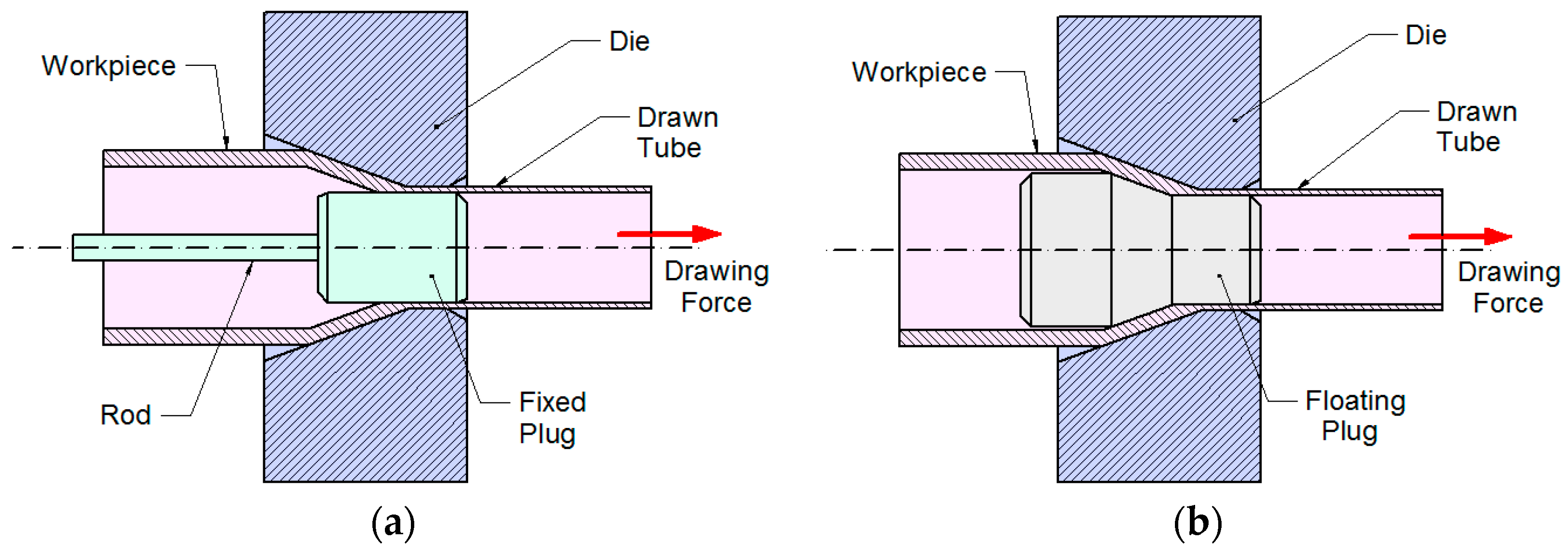
Metallic tubes are usually used in a great number of industrial sectors such as aerospace, defense, medical, transport and nuclear industries, to name but a few. Obtaining such types of pieces, in particular thin-walled ones, usually involves a cold finishing process in which the tube is drawn through a die until its diameter, the thickness of its wall, or both reach values of supply standard [23,24]. Usually, mandrels and plugs are located inside the die in order to achieve a more accurate dimension of the inner diameter of the tube [25]. Figure 1 shows the tube drawing process with a plug, fixed by a rod (a) and floating (b).
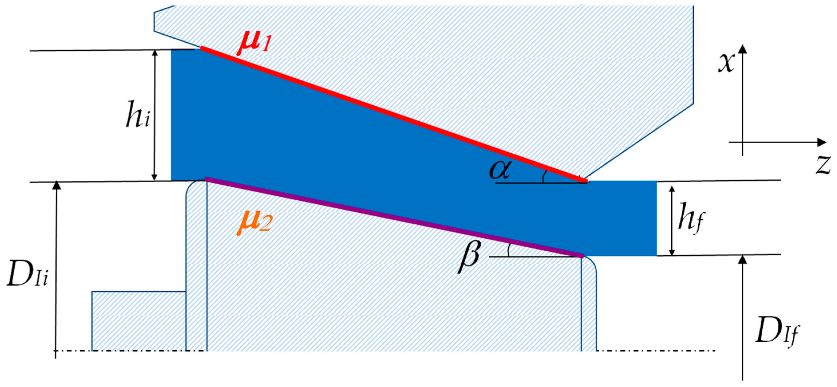
Tube drawing process in convergent conical die with fixed conical inner plug fixed to the draw bench is the process analyzed in this work. The tube inner diameter is going to be considered constant along the process. Then, the initial and final inner diameters ( and , respectively) can be considered constant along the process and of value ( ≈ ≈ ), varying only the thickness from an initial value of to a final one of , as illustrated in Figure 2.
The thin-walled tube drawing process with a fixed conical inner plug can be considered that occurs under plane strain conditions since there is no appreciable variation of its inner diameter ( ≈ ≈ ), as indicated above. According to Hill [26], these conditions represent a material under shear stress state in which the material flow takes place as a result of the denominated shear yield stress, . In addition, a superposed hydrostatic stress, generally of compression, can exist. This stress alters the values of the principal stresses and , but does not influence the material flow [23].
However, the metal at the die exit is free to undergo transverse or circumferential strains, as indicated in several classical handbooks on metal forming and plasticity [27,28,29] because it is in a state of uniaxial stress rather than of plane strain. That makes some authors recommend the plug to be slightly larger than necessary to obtain the precise dimensions of the tube [25] and constitutes the real limit of the tube drawing, since the strength that finally limits the last pass is the uniaxial yield stress, , and no the yield stress under plane strain, . Although the plane strain conditions stay in the real deformation zone, such limit represents the instability of the material under tension and comes given by
where represents the limit of instability of the material under tension (Limit-IMUT).
The process variables related to the geometry are the conical convergent die semiangle , the fixed conical plug semiangle, , place inside of the die; and the tube cross-sectional area reduction, , defined by an equation obtained in a previous work [23].
On the other hand, the existing friction between the interfaces die-tube outer surface and plug-tube inner surface has been considered of Coulomb type and with values of the Coulomb friction coefficients and , respectively.
This paper, focused on the thin-walled tubes drawing processes with a fixed conical inner plug, gives some interesting guidelines to select the plug or set of plugs more adequate to carry out the finishing process described above, considering the tube material, the most relevant geometrical factors of the problem, and the friction conditions. The analysis is carried out by means of the upper bound method (UBM), modelling the plastic deformation zone by triangular rigid zones (TRZ), and considering that the process occurs under plane strain and Coulomb friction conditions. A two-dimensional finite element model is designed to validate the results obtained by the analytical method. In addition, the model has been validated by other finite element method (FEM) simulations and real experiments taken from other researchers found in the literature [30,31] (called literature simulations and literature experimental results, respectively).
2. Methods and Materials
2.1. Analytical Model Based in the Upper Bound Method
The upper bound method has been used to analyze this problem. This method is able to provide a value of the energy required in the process bigger than or equal to the one looked for. Therefore, taking the solution corresponding to the equality a quite approximated estimation is obtained, in many cases, to the solution of the problem.
The UBM application requires the previous modelling of the deformation zone. In this case, three triangular rigid zones (TRZ) have been used [32,33] as it can be seen in Figure 3. For establishing it, different geometric configurations were analyzed in another work of the authors [34], along with its robustness. In that work, it was possible to see that the energy values involved in the tube drawing process, in adimensional terms, are practically independent of the angle ϕ, when dies with small conical semiangles, α, are used, and show certain dispersion for high α values, being the minimum dispersion of the values (smaller than a 7.5%) when ϕ = 30°.
Applying the UBM to the tube drawing process, the following equation is obtained:
where is the necessary power to carry out the process; is the stress at the die exit; and are the diameter and the final thickness of the tube, respectively; is the velocity at the tube exit; is the shear yield stress along the different discontinuity lines; , , , and are the mechanic effects along the discontinuity lines , , , and , respectively; and are the friction effect between the material in the deformation zone and the die along the and ; is the friction effect between the material in the deformation zone and the inner plug along the ; is the relative speed between the i and j blocks (the three triangular ones and the rectangular at the entrance and at the exit of the tube); and, finally, the pressure in the die has been supposed equal to the pressure in the plug and of value , given by the following equation:
Along the history of the analysis of metal forming processes, a great number of equations have been established in order to define the behaviour of work-hardening materials, especially in classical handbooks of mechanical testing [35], key journal articles about time-temperature relations in metals and alloys [36], and flow curves at different temperatures and strain rates [37], but also in handbooks of reference on metal forming [36,37]. In this work, the materials have been approached by theoretical work-hardening materials (TWH), whose effective flow stress-strain equations can be approached by
where is the stress; is the initial yield stress; is the strength coefficient; is the plastic strain; is the work-hardening coefficient; and is a constant of fit. The constant is structure-dependent and is influenced by processing, while is a material property.
Keeping in mind the value of the pressure given by the Equation (4), the symmetry of the problem, the geometric and cinematic relationships that exist between the segments and the relative velocities (Figure 3), and the values of , , , and given, in a general way, as a function of the plastic strain, , by
and, in particular, by
where , , and are the final deformation and the deformation in segments and , respectively. As there are different possible deformation values between and , and between and , in a first approach, the values of and can be calculated as
Equation (3) can be written by means of Equation (13) that represents the adimensional total energy necessary to carry out the process.
In this research, three theoretical work-hardening materials have been used. Namely, the annealed copper UNS C11000, the aluminum UNS A91100 and the stainless steel UNS S34000. Figure 4 shows the flow stress-strain curves for all of them. Both the well-known experimental curves of these materials taken from the literature (literature stress-strain experimental curves) [25,26,27,28,29,32,33,35,36,37,38,39,40,41] and the theoretical ones proposed in this work that, as it can be seen in Figure 4, fit very close to the first ones.
2.2. Numerical Modelling
In order to validate the analytical model presented in this paper, a finite element analysis (FEA) has been carried out. The finite element software used in this analysis is DEFORM (Scientific Forming Technologies Corporation, v11.0, Columbus, OH, USA) [42]. This program is a specific purpose code that is especially designed to simulate both bulk [43] and sheet metal forming processes [44]. The design of the tools (die and mandrel) has been previously developed in AutoCAD (Autodesk Developer Network, 2013, San Rafael, CA, USA) and subsequently imported into DEFORM™-F2. The geometrical parameters considered in the finite element (FE) model are described in Figure 5.
The dimensions of the tube for a cross-sectional area reduction of 10% are presented in Table 3. The length of the tube is 100 mm to guarantee that the process reaches a permanent regime.
DEFORM F2™ is a numerical code of implicit methodology that uses the Newton-Raphson method for solving the equations. The mesh is created by the mesh generator of DEFORM F2™ that consists of a fully automatic, optimized remeshing algorithm [42], and the user only has to define the geometrical complexity and accuracy required for the problem. As indicated in the DEFORM user’s manual [42], the program implements a contact boundary condition with robust remeshing, so the mesh at the contact zone will be remeshed automatically in every case. Considering that tube drawing is not a complex problem from a numerical point of view compared to other problem geometries (for example, extrusion or stamping of complex profiles), a moderate complexity and a moderate to accurate level for accuracy have been chosen. The numerical analysis is developed in 250 steps, and the step increment is defined as 10.
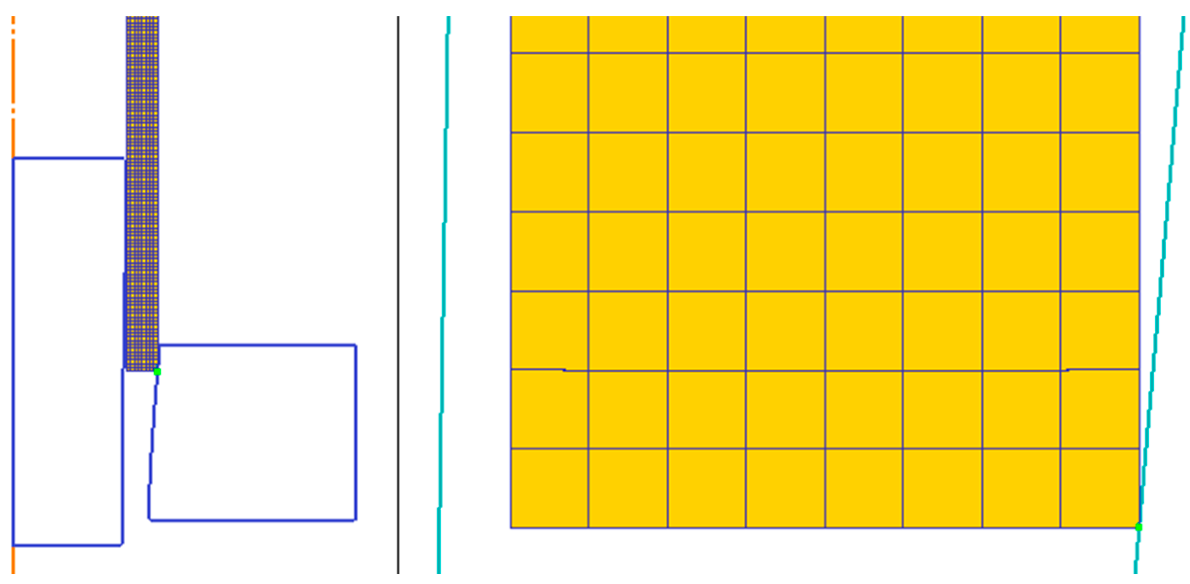
The number of mesh elements in all models is around 2700, with more than 3000 nodes, a number high enough to provide robust results after running several models with different mesh sizes. Considering that the initial wall thickness of the tube is 2.34 mm, that eight mesh elements have been included along the wall thickness of the tube according to our experience and to previous works found in the literature [48], and that the mesh elements are quadrilateral, then the starting mesh size is around 0.3 mm. The tube material considered in the FE model is the alloy UNS C11000 (CDA-110 in DEFORM F2™), and it has been imported from its library.
The configuration of the mesh at the initial step is presented in Figure 6, where it can be seen how the tube is in contact with the die in one single point (a contact line in tridimensional view). In this figure, it can also be appreciated that the workpiece has been meshed with first order continuum elements of quadrilateral shape.
In an industrial drawing process of thin-walled tubes with fixed conical inner plug, both the die and the mandrel remain fixed through the deformation process. Due to the fact that in DEFORM F2™ it is mandatory to assign movement to one of the tools, the boundary conditions imposed consist of constraining the movement in axial direction of the nodes at the tube inlet, and assigning a constant velocity of 50 mm/s in axial direction to the mandrel and the die, a typical value used in industrial applications of this process. This way of modeling boundary conditions is commonly used in simulation of tube drawing by finite element method [46].
3. Results and Discussion
3.1. Theoretical Results
Curves similar to the ones shown in Figure 7 have been plotted for each material and each combination of variables values collected in Table 2 along with its limit for the instability of the material under tension (Limit–IMUT). From these curves, it has been possible to establish for each group of values (, , , ) and material, the set of plugs that make possible to carry out the process, among them, those that make possible to carry out the process under good conditions, and the concrete plug that makes possible to carry out the process using the minimum amount of energy. Such intervals and angles have been collected in Table 4.
3.2. Analytical Model Validation by Finite Element Analysis
Figure 8 shows the comparison of results obtained by finite element analysis (FEA) versus the ones previously obtained by the UBM proposed in this paper. Results for a rigid-perfectly plastic (RPP) material behaviour implemented in the UBM are presented as well in the graphs.
It can be seen that the UBM model with theoretical work-hardening materials (TWH) provides an upper limit of the energy required as all the curves present higher values than the ones obtained by the FE model. Even for a rigid-perfectly plastic (RPP) material, results from FEA are under the UBM model, except in the case of = 5°. It is worth noting that FEA results get closer to the UBM ones in the nearby of optimum. This effect is also noticeable when more extreme conditions are considered (higher cross-sectional area reductions and higher friction conditions), as it is shown in Figure 9, where both methods present very similar results in the proximity of the optimum plug semiangle.
According to this, the UBM model provides results in good agreement with the ones obtained by FEA, and it can be validated as a suitable tool in plug selection for thin-walled tube drawing processes.
3.3. Analytical Model Validation by Literature Results
Additionally, the method has been validated by experimental results taken from external works found in the literature about the theme, called literature results. Concretely, the model of UBM has been validated by FEM simulations (literature simulations) and experimental values (literature experiments) of other authors [30,31].
The material used in these works [30,31], a Ni–Ti shape-memory-alloy (Ni–Ti SMA_LE), has been approximated by a theoretical one (Ni–Ti SMA_T); in the same way that the others used in the present work. The constants of the material are collected in Table 5. This theoretical material has been plotted, in Figure 10, along with the literature experimental material provided in the Yoshida and Furuya’s work [31].
Figure 11 shows the validation of the UBM model given in this work. In this figure, the values obtained with the model of UBM proposed using the same parameters that in the Yoshida and Furuya’s work [31] have been plotted. Table 6 collects the values of σzf/2 k found in the literature. Concretely, in the column 1, the literature FEM simulations values (LFEM); in column 2, the literature experimental ones (LE); and, in the column 3, the obtained results by the UBM model proposed in this work (UBM) using the same parameters values that in the above mentioned work [48]. The parameters values are, concretely, α = 13°, β = 11°, μ1 = 0.10; μ2 = 0.05, and the cross-sectional area reductions r = 0.10, 0.16, and 0.20.
As it is possible to see, the values obtained with the UBM model proposed follow the same trend as those obtained by simulations with other software programs of FEM, different from ours, and with the real experiments (all of them taken from the literature)—being the obtained values from the UBM greater than the other results—as was expected, since this method provides a higher limit [49]. However, the UBM provides the most accurate results in the area of the optimal semiangles, as can be shown in Figure 8 and Figure 9, and it was also observed in previous works focused in plate drawing analysis [50], where UBT provided an upper limit of the energy involved in the process, but the solution was quite accurate for semiangle values next to the optimal semiangles obtained by FEM. Therefore, although the values obtained with the UBM differ from those obtained with other simulation and experimental methods, they can be used to determine the abscissas where the minimums (or intervals around the minimum) of the functions represented are produced; that is, the angles or semi-angles of the plugs or set of plugs that allow the process to be carried out, to be carried out under good conditions or to be carried out under optimum conditions. The method used also provides an upper limit of the energy required in the process, so it also serves to determine the maximum power that will be needed to perform the process and, therefore, will serve to select the machine in which it can be performed. The proposed UBM model is simple and economical to use, since it only requires a spreadsheet for its application while the specific software programs to develop the simulations are usually expensive, require qualified personnel specifically for its management and use longer implementation time. On the other hand, real experiments (not the literature ones used in this work) require specific facilities, certain machines and tools, test tubes of different materials, and qualified personnel for the management and maintenance of all equipment as well as for the analysis of the results. Summarizing, the application of the proposed UBM model is advantageous over other methods for the selection of plugs used in thin-walled tube drawing processes of metallic alloys.
4. Conclusions
This paper, focused on drawing processes of thin-walled tubes carried out with fixed conical inner plugs, gives some practical guidelines to select the plug or set of plugs more adequate to perform the cold finishing process in which the tube is drawn through a die, until that its diameter, the thickness of its wall, or both reach values of supply standard.
The analysis is developed by means of the upper bound method (UBM), modelling the plastic deformation zone by triangular rigid zones (TRZ), and considering that the process occurs under plane strain and Coulomb friction conditions. The UBM has been validated by conducting a finite element analysis (FEA) of different cases under different process conditions and results show a good agreement in all cases.
In addition, the results have been compared with others, both of simulations by finite element method (FEM) and experimental ones, found in the literature about the theme. From this comparison, it can be seen that the results obtained by the UBM follow the same trend, being higher than all of them, as it was expected, since this method provides an upper limit.
The study has allowed establishing for each material and combination of the variables and of the friction conditions a first set of plugs that allows carrying out the process (PS1), a second set of plugs that allow carrying out the process under good conditions in terms of energy consumption (PS2), and the optimum plug that makes possible to carry out the process using the minimum amount of energy (OP). Therefore, the best would be selecting the optimum plug in order to perform the process with the lower energy as possible. However, in the shop-floors all the plugs are not always available since they are very costly, and they are not bought in all sizes or, even although there are among the resources of the shop-floor, in this moment, it can be possible that they are being repaired or under maintenance. Then, in many cases, it will be necessary to use other available plugs to obtain the products to satisfy the customers in the agree deadlines. The guideline step to step to select the most adequate plug in each case is
- ▪
- Check the angle (or semiangle) of the available dies in the shop-floor.
- ▪
- Select the cross-sectional area reduction to manufacture tubes with the required dimensions.
- ▪
- Select the material of the tube.
- ▪
- Select the values of the Coulomb friction coefficients (die-tube and tube-plug).
- ▪
- Select the optimum plug (value found in the third column of the selected material).
- ▪
- Check if there is in the shop-floor a plug with the geometry indicated. If the answer is yes, this is the plug to use but, if not, it is necessary to continue.
- ▪
- Select the second column, that is, the plugs set that allows carrying out the process under good conditions in terms of energy consumption.
- ▪
- Check if there are in the shop-floor some plugs with the geometries indicated in the second column. If the answer is yes, these are the plugs to use but, if not, it is necessary to continue.
- ▪
- Select the first column, that is, the plugs set that allows carrying out the process.
Check if there are some plugs in the shop-floor with the geometries indicated in the first column. If the answer is yes, these are the plugs to use; if not, it will not be possible to carry out the process in the shop-floor. Then, to carry out the process, it is necessary to buy a plug (if possible, the optimum one).
From the analysis of the behaviour of all them, it is possible to establish that the plug that allows carrying out the process with minimum quantity of energy is cylindrical in most cases ( = 0°), being conical only for low (0.10) and medium (0.20) cross-sectional area reductions and certain combinations of the Coulomb friction coefficients ( and ) for die semiangles, , bigger than 10°.
Practical applications of the tube drawing processes can be improved with this study since it provides, in a simple and economic way, an adequate and enough knowledge for technological decision-making based in the energy required to carry out the process; such as machines, dies and, in particular, about the plug selection.
Acknowledgments
This work has been financially supported by funds provided through the Annual Grants Call of the E.T.S.I.I. of UNED through the projects of references 2017-ICF04, 2017-ICF05, and 2017-ICF08. The authors would like to take this opportunity to thank the Research Group of the UNED “Industrial Production and Manufacturing Engineering (IPME)” for the support provided during the development of this work. Especially, to Miguel A. Sebastián (UNED) for the helpful suggestions that he has made during this research.
Author Contributions
Eva María Rubio, Ana María Camacho, and Raúl Pérez conceived and designed the study; Eva María Rubio and Marta María Marín developed the UBM model; Ana María Camacho and Raúl Pérez developed the finite element model; Eva María Rubio, Ana María Camacho, Raúl Pérez, and Marta María Marín analyzed the data; Eva María Rubio, Ana María Camacho, and Raúl Pérez wrote the paper.
Conflicts of Interest
The authors declare no conflict of interest.
References
- Celentano, D.J.; Palacios, M.A.; Rojas, E.L.; Cruchaga, M.A.; Artigas, A.A.; Monsalve, A.E. Simulation and experimental validation of multiple-step wire drawing processes. Finite Elem. Anal. Des. 2009, 45, 163–180. [Google Scholar] [CrossRef]
- Camacho, A.M.; Domingo, R.; Rubio, E.; González, C. Analysis of the influence of back-pull in drawing process by the finite element method. J. Mater. Process. Technol. 2005, 164–165, 1167–1174. [Google Scholar] [CrossRef]
- Rubio, E.M.; Camacho, A.M.; Sevilla, L.; Sebastián, M.A. Calculation of the forward tension in drawing processes. J. Mater. Process. Technol. 2005, 162–163, 551–557. [Google Scholar] [CrossRef]
- Vega, G.; Haddi, A.; Imad, A. Investigation of process parameters effect on the copper-wire drawing. Mater. Des. 2009, 30, 3308–3312. [Google Scholar] [CrossRef]
- Camacho, A.M.; González, C.; Rubio, E.M.; Sebastián, M.A. Influence of geometrical conditions on central burst appearance in axisymmetrical drawing processes. J. Mater. Process. Technol. 2006, 177, 304–306. [Google Scholar] [CrossRef]
- McAllen, P.J.; Phelan, P. Numerical analysis of axisymmetric wire drawing by means of a coupled damage model. J. Mater. Process. Technol. 2007, 183, 210–218. [Google Scholar] [CrossRef]
- Weygand, S.M.; Riedel, H.; Eberhard, B.; Wouters, G. Numerical simulation of the drawing process of tungsten wires. Int. J. Refract. Met. Hard Mater. 2006, 24, 338–342. [Google Scholar] [CrossRef]
- Haddi, A.; Imad, A.; Vega, G. Analysis of temperature and speed effects on the drawing stress for improving the wire drawing process. Mater. Des. 2011, 32, 4310–4315. [Google Scholar] [CrossRef]
- Lambiase, F.; Di Ilio, A. Deformation inhomogeneity in roll drawing process. J. Manuf. Process. 2012, 14, 208–215. [Google Scholar] [CrossRef]
- Panteghini, A.; Genna, F. Effects of the strain-hardening law in the numerical simulation of wire drawing processes. Comput. Mater. Sci. 2010, 49, 236–242. [Google Scholar] [CrossRef]
- Toribio, J.; Lorenzo, M.; Vergara, D. Hydrogen embrittlement susceptibility of prestressing steel wires: The role of the cold-drawing conditions. Procedia Struct. Integr. 2016, 2, 626–631. [Google Scholar] [CrossRef]
- Toribio, J.; Lorenzo, M.; Vergara, D.; Aguado, L. Residual stress redistribution induced by fatigue in cold-drawn prestressing steel wires. Constr. Build. Mater. 2016, 114, 317–322. [Google Scholar] [CrossRef]
- Toribio, J.; Lorenzo, M.; Vergara, D.; Aguado, L. The role of overloading on the reduction of residual stress by cyclic loading in cold-drawn prestressing steel wires. Appl. Sci. 2017, 7, 84. [Google Scholar] [CrossRef]
- Ripoll, M.R.; Weygand, S.M.; Riedel, H. Reduction of tensile residual stresses during the drawing process of tungsten wires. Mater. Sci. Eng. A 2010, 527, 3064–3072. [Google Scholar] [CrossRef]
- Toribio, J.; Lorenzo, M.; Vergara, D.; Kharin, V. Influence of the die geometry on the hydrogen embrittlement susceptibility of cold drawn wires. Eng. Fail. Anal. 2014, 36, 215–225. [Google Scholar] [CrossRef]
- Baek, H.M.; Jin, Y.G.; Hwang, S.K.; Im, Y.-T.; Son, I.-H.; Lee, D.-L. Numerical study on the evolution of surface defects in wire drawing. J. Mater. Process. Technol. 2012, 212, 776–785. [Google Scholar] [CrossRef]
- Felder, E.; Levrau, C. Analysis of the lubrication by a pseudoplastic fluid: Application to wire drawing. Tribol. Int. 2011, 44, 845–849. [Google Scholar] [CrossRef]
- Bermudo, C.; Sevilla, L.; Martín, F.; Trujillo, F. Study of the tool geometry influence in indentation for the analysis and validation of the new modular upper bound technique. Appl. Sci. 2016, 6, 203. [Google Scholar] [CrossRef]
- Lowrie, J.; Ngaile, G. Analytical modeling of hydrodynamic lubrication in a multiple-reduction drawing die. J. Manuf. Process. 2017, 27, 291–303. [Google Scholar] [CrossRef]
- Lei, X.; Dong, L.; Zhang, Z.; Liu, Y.; Hao, Y.; Yang, R.; Zhang, L.-C. Microstructure, texture evolution and mechanical properties of VT3-1 titanium alloy processed by multi-pass drawing and subsequent isothermal annealing. Metals 2017, 7, 131. [Google Scholar] [CrossRef]
- Juul, K.J.; Nielsen, K.L.; Niordson, C.F. Steady-state numerical modeling of size effects in micron scale wire drawing. J. Manuf. Process. 2017, 25, 163–171. [Google Scholar] [CrossRef]
- Filice, L.; Ambrogio, G.; Guerriero, F. A multi-objective approach for wire-drawing process. Procedia CIRP 2013, 12, 294–299. [Google Scholar] [CrossRef]
- Rubio, E.M. Analytical methods application to the study of tube drawing processes with fixed conical inner plug: Slab and Upper Bound Methods. J. Achiev. Mater. Manuf. Eng. 2006, 14, 119–130. [Google Scholar]
- Rubio, E.M.; Marín, M.; Domingo, R.; Sebastián, M.A. Analysis of plate drawing processes by the upper bound method using theoretical work-hardening materials. Int. J. Adv. Manuf. Technol. 2009, 40, 261–269. [Google Scholar] [CrossRef]
- Avitzur, B. Handbook of Metal Forming Processes; John Wiley & Sons: New York, NY, USA, 1983; ISBN 978-0471034742. [Google Scholar]
- Hill, R. The Mathematical Theory of Plasticity; Oxford University Press: London, UK, 1950. [Google Scholar]
- Rowe, G.W. Elements of Metalworking Theory; Edward Arnold: London, UK, 1979. [Google Scholar]
- Hoffman, O.; Sachs, G. Introduction to the Theory of Plasticity for Engineers; McGraw-Hill Book Company Inc.: New York, NY, USA, 1953. [Google Scholar]
- Slater, R.A.C. Engineering Plasticity: Theory and Application to Metal Forming Processes; The Macmillan Press Ltd.: London, UK, 1977; ISBN 9780333157091. [Google Scholar]
- Yoshida, K.; Watanabe, M.; Ishikawa, H. Drawing of Ni-Ti shape-memory-alloy fine tubes used in medical tests. J. Mater. Process. Technol. 2001, 118, 251–255. [Google Scholar] [CrossRef]
- Yoshida, K.; Furuya, H. Mandrel drawing and plug drawing of shape-memory-alloy fine tubes used in catheters and stents. J. Mater. Process. Technol. 2004, 153–154, 145–150. [Google Scholar] [CrossRef]
- Avitzur, B. Metal Forming: The Application of Limit Analysis; Marcel Dekker: New York, NY, USA, 1980. [Google Scholar]
- Talbert, S.H.; Avitzur, B. Element Mechanics of Plastic Flow in Metal Forming; John Wiley & Sons: New York, NY, USA, 1996; ISBN 9780471960034. [Google Scholar]
- Rubio, E.M.; Camacho, A.M.; Pérez, R.; Marín, M. Modelo mejorado de bloques rígidos triangulares para el análisis mediante el método del límite superior de procesos de estirado de tubos con tapón interior cónico fijo. In Actas del XXII Congreso Nacional de Ingeniería Mecánica; Asociación Española de Ingeniería Mecánica: Madrid, Spain, 2018. [Google Scholar]
- Kuhn, H.; Medlin, D. ASM Handbook Volume 8: Mechanical Testing and Evaluation; ASM International Metals Parks: Materials Park, OH, USA, 2000; ISBN 9780871703897. [Google Scholar]
- Hollomon, J.H.; Jaffe, L.D. Time-temperature relations in tempering steel. Trans. Am. Inst. Min. Metall. Eng. 1945, 162, 223–249. [Google Scholar]
- Rao, K.P.; Doraivelu, S.M.; Gopinathan, V. Flow curves and deformation of materials at different temperatures and strain rates. J. Mech. Work. Technol. 1982, 6, 63–88. [Google Scholar] [CrossRef]
- Hosford, W.F.; Caddell, R.M. Metal Forming: Mechanics and Metallurgy; Cambridge University Press: New York, NY, USA, 2007; ISBN 9780521881210. [Google Scholar]
- Johnson, W.; Mellor, P.B. Engineering Plasticity; Ellis Horwood: Chichester, UK, 1983. [Google Scholar]
- Roylance, D. Stress-Stain Curves; Department of Materials Science and Engineering, Massachusets Institute of Tecnology: Cambrige, MA, USA, 2001. [Google Scholar]
- Kalpakjian, S.; Schmid, S.R. Manufacturing Processes for Engineering Materials, 5th ed.; Prentice-Hall/Pearson Education: Upper Saddle River, NJ, USA, 2008. [Google Scholar]
- Corporation, S.F.T. DEFORM-F2 v11.0 User’s Manual; Scientific Forming Technologies Corporation: Columbus, OH, USA, 2014. [Google Scholar]
- Amigo, F.J.; Camacho, A.M. Reduction of induced central damage in cold extrusion of dual-phase steel DP800 using double-pass dies. Metals 2017, 7, 335. [Google Scholar] [CrossRef]
- Centeno, G.; Martínez-Donaire, A.; Bagudanch, I.; Morales-Palma, D.; Garcia-Romeu, M.; Vallellano, C. Revisiting formability and failure of AISI304 sheets in spif: Experimental approach and numerical validation. Metals 2017, 7, 531. [Google Scholar] [CrossRef]
- Neves, F.O.; Button, S.T.; Caminaga, C.; Gentile, F.C. Numerical and experimental analysis of tube drawing with fixed plug. J. Braz. Soc. Mech. Sci. Eng. 2005, 27, 426–431. [Google Scholar] [CrossRef]
- Danckert, J.; Endelt, B. LS-DYNA® used to analyze the drawing of precision tubes. In Proceedings of the 7th European LS-DYNA Conference, Salzburg, Germany, 14–15 May 2009. [Google Scholar]
- Świątkowski, K.; Hatalak, R. Application of modified tools in the process of thin-walled tube drawing. Arch. Metall. Mater. 2006, 51, 193–197. [Google Scholar]
- Palengat, M.; Chagnon, G.; Favier, D.; Louche, H.; Linardon, C.; Plaideau, C. Cold drawing of 316L stainless steel thin-walled tubes: Experiments and finite element analysis. Int. J. Mech. Sci. 2013, 70, 69–78. [Google Scholar] [CrossRef] [Green Version]
- Martín, F.; Camacho, A.M.; Domingo, R.; Sevilla, L. Modular procedure to improve the application of the upper-bound theorem in forging. Mater. Manuf. Process. 2013, 28, 282–286. [Google Scholar] [CrossRef]
- Camacho, A.M.; Rubio, E.M.; González, C.; Sebastián, M.A. Study of drawing processes by analytical and finite element methods. Mater. Sci. Forum 2006, 526, 187–192. [Google Scholar] [CrossRef]
Figure 1.
Tube drawing process with (a) a fixed plug and (b) a floating plug.

Figure 2.
Detail of the plastic deformation zone.

Figure 3.
Modelling of the plastic deformation zone with three triangular rigid zones.
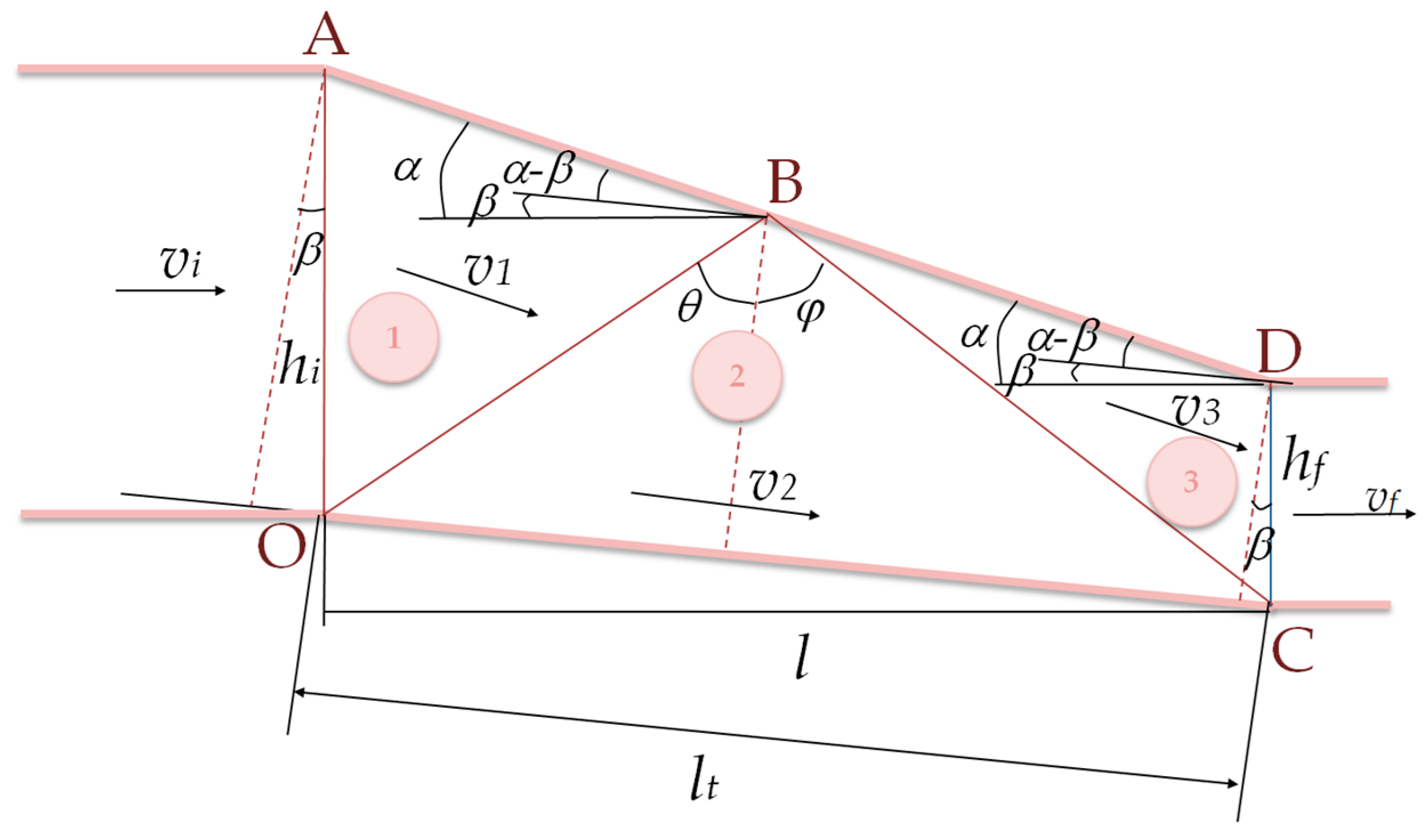
Figure 4.
Literature experimental (LE) and theoretical (T) effective flow stress-strain curves for annealed copper UNS C11000, aluminum UNS A91100, and stainless steel UNS S34000.
Figure 4.
Literature experimental (LE) and theoretical (T) effective flow stress-strain curves for annealed copper UNS C11000, aluminum UNS A91100, and stainless steel UNS S34000.
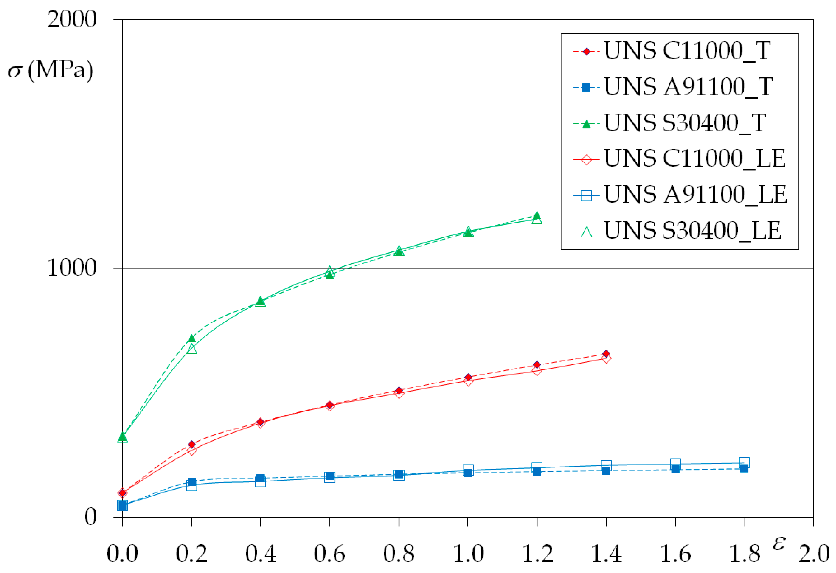
Figure 5.
Geometrical parameters implemented in the finite element (FE) model.
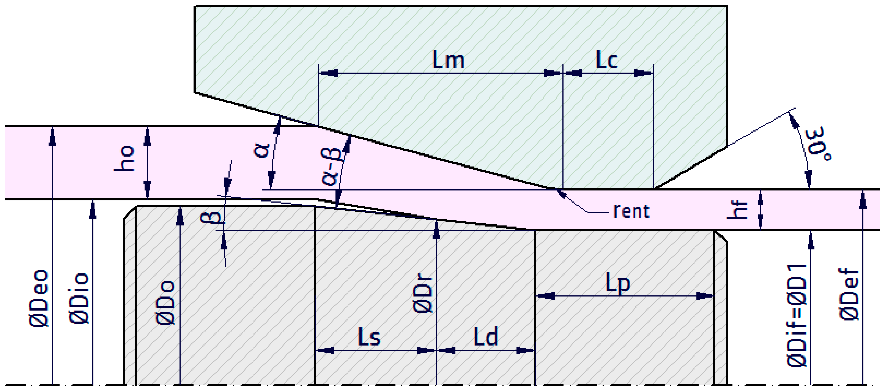
Figure 6.
Mesh at initial step and detail of contact between tube and die.

Figure 7.
Adimensional total energy calculated for = 5°, = 0.10, = 0.05, = 0.25, along with the instability limit of the material under tension (Limit-IMUT) for (a) copper UNS C11000, (b) aluminium UNS A91100, and (c) stainless steel UNS S34000.
Figure 7.
Adimensional total energy calculated for = 5°, = 0.10, = 0.05, = 0.25, along with the instability limit of the material under tension (Limit-IMUT) for (a) copper UNS C11000, (b) aluminium UNS A91100, and (c) stainless steel UNS S34000.

Figure 8.
Validation of UBM model by FEA for different die semiangles and fixed conical plug semiangles ( = 0.10; = 0.05; = 0.05; and copper alloy UNS C11000) and their corresponding effective stress contour diagrams obtained by DEFORM for = 0°: (a) α = 5°; (b) α = 10°; (c) α = 15°; and (d) α = 20°.

Figure 9.
Validation of upper bound method (UBM) model by finite element analysis (FEA) varying other parameters and corresponding effective stress contour diagrams obtained by DEFORM for = 0°: (a) α = 5°; = 0.40; = = 0.05; (b) α = 20°; = 0.10; = = 0.20.
Figure 9.
Validation of upper bound method (UBM) model by finite element analysis (FEA) varying other parameters and corresponding effective stress contour diagrams obtained by DEFORM for = 0°: (a) α = 5°; = 0.40; = = 0.05; (b) α = 20°; = 0.10; = = 0.20.
Figure 10.
Literature experimental (LE) and theoretical (T) effective flow stress-strain curves for the Ni-Ti shape-memory alloy.
Figure 10.
Literature experimental (LE) and theoretical (T) effective flow stress-strain curves for the Ni-Ti shape-memory alloy.

Figure 11.
UBM model validation by literature FEM simulations (LFEM) and literature experimental values (LE) taken as parameters values: r = 10–20%; α = 13°; β = 11°; μ1 = 0.10; μ2 = 0.05 [48].
Figure 11.
UBM model validation by literature FEM simulations (LFEM) and literature experimental values (LE) taken as parameters values: r = 10–20%; α = 13°; β = 11°; μ1 = 0.10; μ2 = 0.05 [48].

| Parameters | Materials | ||
|---|---|---|---|
| UNS C11000 | UNS A91100 | UNS S34000 | |
| (MPa) | 100 | 50 | 320 |
| (MPa) | 315 | 180 | 1275 |
| 0.54 | 0.20 | 0.45 | |
| 1.5 | −1.0 | −1.4 | |
Table 2.
Ranges of values used in the calculation of the total energy.
| (°) | (°) | |||
|---|---|---|---|---|
| 5 | 1–4 | 0.10–0.40 | 0–0.25 | 0–0.25 |
| 10 | 1–9 | |||
| 15 | 1–14 | |||
| 20 | 1–19 |
Table 3.
Tube dimensions (in mm) for = 0.1.
| 22.00 | 20.76 | 17.32 | 16.55 | 2.34 | 2.11 |
Table 4.
PS 1: plugs set that allow carrying out the process; PS 2: plugs set that allow carrying out the process under good conditions in terms of energy consumption; and OP: optimum plug that makes it possible to carry out the process using the minimum amount of energy.
Table 4.
PS 1: plugs set that allow carrying out the process; PS 2: plugs set that allow carrying out the process under good conditions in terms of energy consumption; and OP: optimum plug that makes it possible to carry out the process using the minimum amount of energy.
| (°) | (°) | |||||||||||
|---|---|---|---|---|---|---|---|---|---|---|---|---|
| UNS A91100 | UNS S34000 | UNS C11000 | ||||||||||
| PS 1 | PS 2 | OP | PS 1 | PS 2 | OP | PS 1 | PS 2 | OP | ||||
| 5 | 0.1 | 0.05 | 0.05 | 0–4 | 0–1 | 0 | 0–4 | 0–2 | 0 | 0–4 | 0–2 | 0 |
| 0.05 | 0.25 | 0–3 | 0–1 | 0 | 0–3 | 0–2 | 0 | 0–3 | 0–2 | 0 | ||
| 0.25 | 0.05 | 0–4 | 0–2 | 0 | 0–4 | 0–3 | 0 | 0–4 | 0–3 | 0 | ||
| 0.25 | 0.25 | 0–3 | 0–1 | 0 | 0–4 | 0–2 | 0 | 0–3 | 0–2 | 0 | ||
| 0.2 | 0.05 | 0.05 | 0–3 | 0–1 | 0 | 0–3 | 0–1 | 0 | 0–3 | 0–1 | 0 | |
| 0.05 | 0.25 | 0–1 | 0–1 | 0 | 0–2 | 0–1 | 0 | 0–1 | 0–1 | 0 | ||
| 0.25 | 0.05 | 0–3 | 0–1 | 0 | 0–3 | 0–1 | 0 | 0–3 | 0–1 | 0 | ||
| 0.25 | 0.25 | 0–1 | 0–1 | 0 | 0–2 | 0–1 | 0 | 0–2 | 0–1 | 0 | ||
| 0.3 | 0.05 | 0.05 | 0–1 | 0–1 | 0 | 0–1 | 0–1 | 0 | 0–2 | 0–1 | 0 | |
| 0.05 | 0.25 | 0–2 | 0–1 | 0 | - | - | - | - | - | - | ||
| 0.25 | 0.05 | 0–2 | 0–1 | 0 | 0–2 | 0–1 | 0 | 0–2 | 0–1 | 0 | ||
| 0.25 | 0.25 | - | - | - | - | - | - | - | - | - | ||
| 0.4 | 0.05 | 0.05 | - | - | - | - | - | - | 0–1 | 0–1 | 0 | |
| 0.05 | 0.25 | - | - | - | - | - | - | - | - | - | ||
| 0.25 | 0.05 | - | - | - | 0–0.5 | 0–0.5 | 0 | - | - | - | ||
| 0.25 | 0.25 | - | - | - | - | - | - | - | - | - | ||
| 10 | 0.1 | 0.05 | 0.05 | 0–9 | 0–5 | 2 | 0–9 | 0–6 | 3 | 0–9 | 0–5 | 3 |
| 0.05 | 0.25 | 0–8 | 0–2 | 0 | 0–8 | 0–3 | 0 | 0–8 | 0–3 | 0 | ||
| 0.25 | 0.05 | 0–8 | 0–6 | 2 | 0–8 | 0–4 | 0 | 0–8 | 0–6 | 3 | ||
| 0.25 | 0.25 | 0–8 | 0–3 | 0 | 0–8 | 0–4 | 0 | 0–8 | 0–3 | 0 | ||
| 0.2 | 0.05 | 0.05 | 0–8 | 0–2 | 0 | 0–8 | 0–2 | 0 | 0–8 | 0–2 | 0 | |
| 0.05 | 0.25 | 0–1 | 0–1 | 0 | 0–6 | 0–2 | 0 | 0–6 | 0–2 | 0 | ||
| 0.25 | 0.05 | 0–8 | 0–3 | 0 | 0–8 | 0–3 | 0 | 0–8 | 0–3 | 0 | ||
| 0.25 | 0.25 | 0–6 | 0–2 | 0 | 0–7 | 0–2 | 0 | 0–6 | 0–2 | 0 | ||
| 0.3 | 0.05 | 0.05 | 0–6 | 0–2 | 0 | 0–7 | 0–2 | 0 | 0–7 | 0–2 | 0 | |
| 0.05 | 0.25 | 0–2 | 0–1 | 0 | 0–4 | 0–1 | 0 | 0–4 | 0–1 | 0 | ||
| 0.25 | 0.05 | 0–6 | 0–2 | 0 | 0–7 | 0–2 | 0 | 0–7 | 0–2 | 0 | ||
| 0.25 | 0.25 | 0–3 | 0–1 | 0 | 0–5 | 0–2 | 0 | 0–4 | 0–2 | 0 | ||
| 0.4 | 0.05 | 0.05 | 0–8 | 0–3 | 0 | 0–4 | 0–2 | 0 | 0–5 | 0–2 | 0 | |
| 0.05 | 0.25 | - | - | - | - | - | - | 0–1 | 0–1 | 0 | ||
| 0.25 | 0.05 | 0–4 | 0–2 | 0 | 0–5 | 0–2 | 0 | 0–5 | 0–2 | 0 | ||
| 0.25 | 0.25 | - | - | - | 0–2 | 0–1 | 0 | 0–2 | 0–1 | 0 | ||
| 15 | 0.1 | 0.05 | 0.05 | 0–14 | 0–11 | 7 | 0–14 | 4–12 | 8 | 0–14 | 4–10 | 8 |
| 0.05 | 0.25 | 0–13 | 0–5 | 0 | 0–13 | 4–10 | 8 | 0–13 | 4–10 | 8 | ||
| 0.25 | 0.05 | 0–14 | 0–11 | 7 | 0–14 | 7–11 | 9 | 0–14 | 0–11 | 7 | ||
| 0.25 | 0.25 | 0–13 | 0–7 | 0 | 0–13 | 3–6 | 4 | 0–13 | 0–7 | 0 | ||
| 0.2 | 0.05 | 0.05 | 0–13 | 0–5 | 0 | 0–13 | 0–5 | 3 | 0–13 | 0–5 | 0 | |
| 0.05 | 0.25 | 0–10 | 0–2 | 0 | 0–11 | 0–4 | 0 | 0–10 | 0–2 | 0 | ||
| 0.25 | 0.05 | 0–13 | 0–7 | 0 | 0–13 | 0–6 | 2 | 0–13 | 0–7 | 0 | ||
| 0.25 | 0.25 | 0–11 | 0–2 | 0 | 0–11 | 0–5 | 0 | 0–11 | 0–2 | 0 | ||
| 0.3 | 0.05 | 0.05 | 0–11 | 0–2 | 0 | 0–11 | 0–4 | 0 | 0–11 | 0–4 | 0 | |
| 0.05 | 0.25 | 0–6 | 0–2 | 0 | 0–8 | 0–2 | 0 | 0–10 | 0–2 | 0 | ||
| 0.25 | 0.05 | 0–11 | 0–4 | 0 | 0–11 | 0–3 | 0 | 0–12 | 0–5 | 0 | ||
| 0.25 | 0.25 | 0–7 | 0–2 | 0 | 0–9 | 0–3 | 0 | 0–8 | 0–4 | 0 | ||
| 0.4 | 0.05 | 0.05 | 0–8 | 0–2 | 0 | 0–8 | 0–3 | 0 | 0–10 | 0–2 | 0 | |
| 0.05 | 0.25 | 0–2 | 0–1 | 0 | 0–4 | 0–2 | 0 | 0–6 | 0–2 | 0 | ||
| 0.25 | 0.05 | 0–9 | 0–3 | 0 | 0–9 | 0–3 | 0 | 0–6 | 0–3 | 0 | ||
| 0.25 | 0.25 | 0–4 | 0–2 | 0 | 0–6 | 0–2 | 0 | 0–6 | 0–2 | 0 | ||
| 20 | 0.1 | 0.05 | 0.05 | 0–19 | 10–16 | 14 | 0–19 | 10–16 | 13 | 0–19 | 10–16 | 12 |
| 0.05 | 0.25 | 0–18 | 0–16 | 8 | 0–18 | 5–11 | 8 | 0–18 | 0–12 | 4 | ||
| 0.25 | 0.05 | 0–19 | 10–16 | 14 | 0–19 | 10–16 | 12 | 0–19 | 8–16 | 12 | ||
| 0.25 | 0.25 | 0–18 | 6–14 | 9 | 0–18 | 3–13 | 9 | 0–18 | 0–12 | 6 | ||
| 0.2 | 0.05 | 0.05 | 0–17 | 4–12 | 9 | 0–18 | 3–11 | 7 | 0–18 | 4–11 | 6 | |
| 0.05 | 0.25 | 0–16 | 0–6 | 0 | 0–16 | 0–6 | 0 | 0–16 | 0–6 | 0 | ||
| 0.25 | 0.05 | 0–17 | 0–13 | 8 | 0–17 | 5–10 | 8 | 0–18 | 0–14 | 6 | ||
| 0.25 | 0.25 | 0–16 | 0–9 | 0 | 0–16 | 0–8 | 0 | 0–16 | 0–8 | 0 | ||
| 0.3 | 0.05 | 0.05 | 0–15 | 0–10 | 0 | 0–15 | 0–5 | 0 | 0–16 | 0–7 | 0 | |
| 0.05 | 0.25 | 0–15 | 0–9 | 0 | 0–12 | 0–5 | 0 | 0–13 | 0–5 | 0 | ||
| 0.25 | 0.05 | 0–11 | 0–4 | 0 | 0–15 | 0–6 | 1 | 0–16 | 0–8 | 0 | ||
| 0.25 | 0.25 | 0–13 | 0–6 | 0 | 0–13 | 0–6 | 0 | 0–13 | 0–6 | 0 | ||
| 0.4 | 0.05 | 0.05 | 0–13 | 0–5 | 0 | 0–13 | 0–6 | 0 | 0–15 | 0–5 | 0 | |
| 0.05 | 0.25 | 0–8 | 0–4 | 0 | 0–8 | 0–3 | 0 | 0–9 | 0–3 | 0 | ||
| 0.25 | 0.05 | 0–13 | 0–7 | 0 | 0–13 | 0–5 | 0 | 0–14 | 0–6 | 0 | ||
| 0.25 | 0.25 | 0–10 | 0–4 | 0 | 0–10 | 0–5 | 0 | 0–11 | 0–4 | 0 | ||
Table 5.
Values of , , , and for the Ni–Ti shape-memory-alloy theoretical material used in the comparison with literature experimental results.
Table 5.
Values of , , , and for the Ni–Ti shape-memory-alloy theoretical material used in the comparison with literature experimental results.
| Parameters | Material |
|---|---|
| Ni–Ti-SMA_T | |
| (MPa) | 400 |
| (MPa) | 1750 |
| 0.95 | |
| 1.85 |
Table 6.
σzf/2 k values. Column 1 by literature FEM simulations (LFEM), column 2 by literature experiments (LE), and column 3 by upper bound method (UBM).
Table 6.
σzf/2 k values. Column 1 by literature FEM simulations (LFEM), column 2 by literature experiments (LE), and column 3 by upper bound method (UBM).
| α = 13°; β = 11°; μ1 = 0.10; μ2 = 0.05 | |||
|---|---|---|---|
| r | σzf/2 k LFEM | σzf/2 k LE | σzf/2 k UBM |
| 0.10 | 0.350 | 0.300 | 1.035 |
| 0.16 | 0.550 | 0.450 | 1.130 |
| 0.20 | 0.650 | 0.800 | 1.192 |
© 2017 by the authors. Licensee MDPI, Basel, Switzerland. This article is an open access article distributed under the terms and conditions of the Creative Commons Attribution (CC BY) license (http://creativecommons.org/licenses/by/4.0/).
Share and Cite
MDPI and ACS Style
Rubio, E.M.; Camacho, A.M.; Pérez, R.; Marín, M.M. Guidelines for Selecting Plugs Used in Thin-Walled Tube Drawing Processes of Metallic Alloys. Metals 2017, 7, 572. https://doi.org/10.3390/met7120572
AMA Style
Rubio EM, Camacho AM, Pérez R, Marín MM. Guidelines for Selecting Plugs Used in Thin-Walled Tube Drawing Processes of Metallic Alloys. Metals. 2017; 7(12):572. https://doi.org/10.3390/met7120572
Chicago/Turabian StyleRubio, Eva María, Ana María Camacho, Raúl Pérez, and Marta María Marín. 2017. "Guidelines for Selecting Plugs Used in Thin-Walled Tube Drawing Processes of Metallic Alloys" Metals 7, no. 12: 572. https://doi.org/10.3390/met7120572
Note that from the first issue of 2016, this journal uses article numbers instead of page numbers. See further details here.