
Effects of EMS Induced Flow on Solidification and Solute Transport in Bloom Mold


Abstract
:1. Introduction
2. Model Descriptions
2.1. Basic Assumptions
- (1)
- The transport phenomena in the mold are assumed to be at steady state and the influence of inclusions on the fluid flow, heat transfer, and species transport is neglected to simplify the simulation.
- (2)
- The impact of fluid flow on the internal heat transfer of molten steel is ignored in this model, and the liquid steel is assumed to be an incompressible Newtonian fluid. The influence of mold oscillation and mold taper on the fluid flow is also ignored.
- (3)
- The effect of thermal contraction on the fluid flow and temperature field in the bloom is neglected.
- (4)
- The mold arc is neglected, and the computational zone is assumed to be a vertical model.
- (5)
- The effect of the melt flow on the electromagnetic field is ignored due to the small magnetic Reynolds number (about 0.01) in the stirring process.
2.2. Governing Equations
2.2.1. Turbulent Flow
2.2.2. Heat Transfer Model
2.2.3. Solute Transport Model
2.2.4. Electromagnetism Model
2.2.5. VOF Model
3. Simulation Procedure and Verification
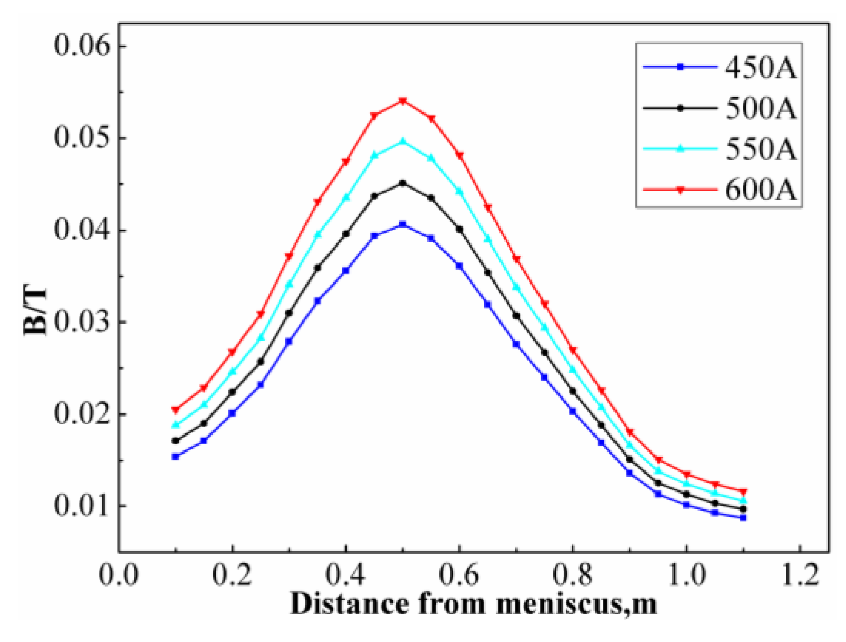
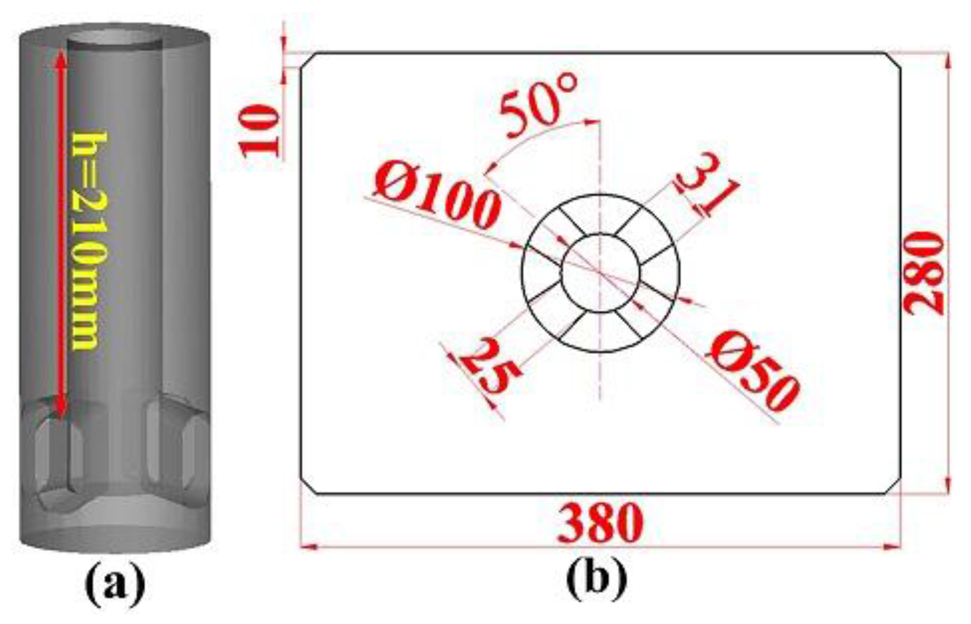
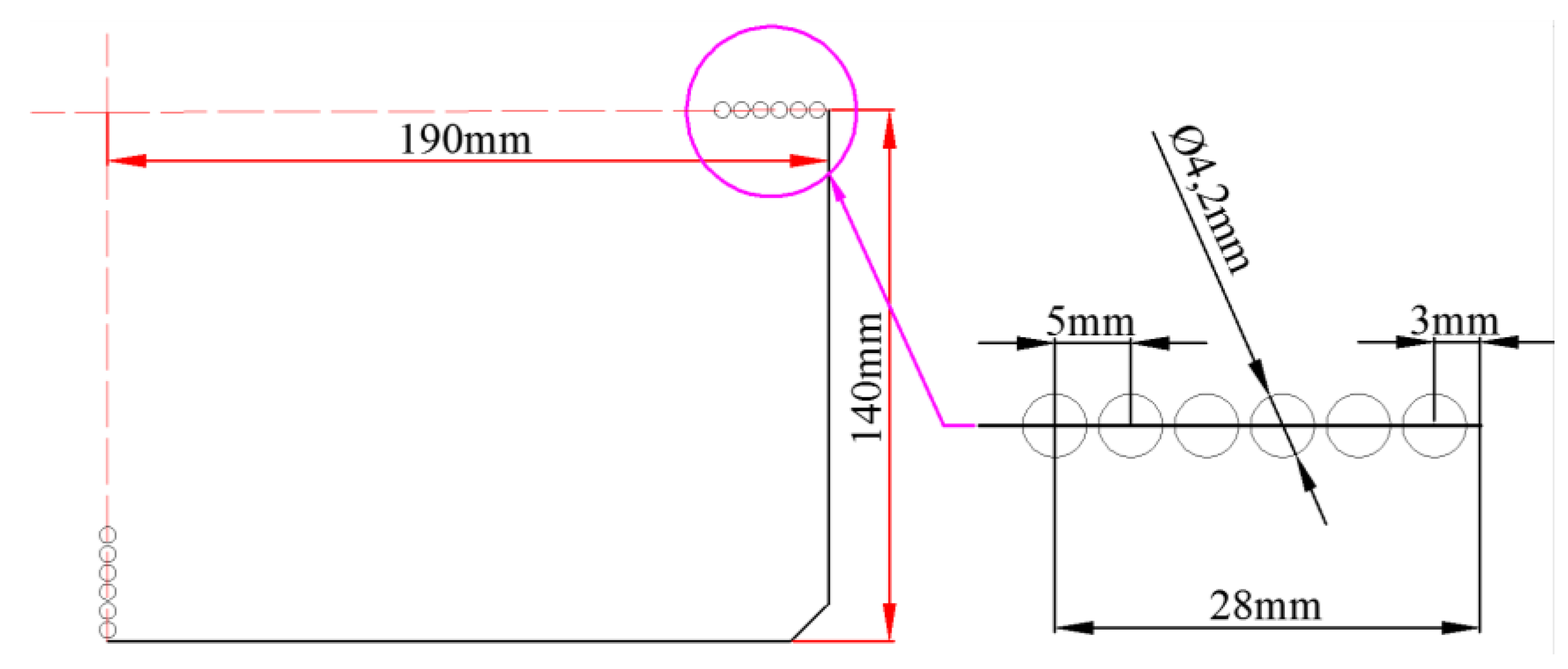
3.1. Operating Condition and Parameters
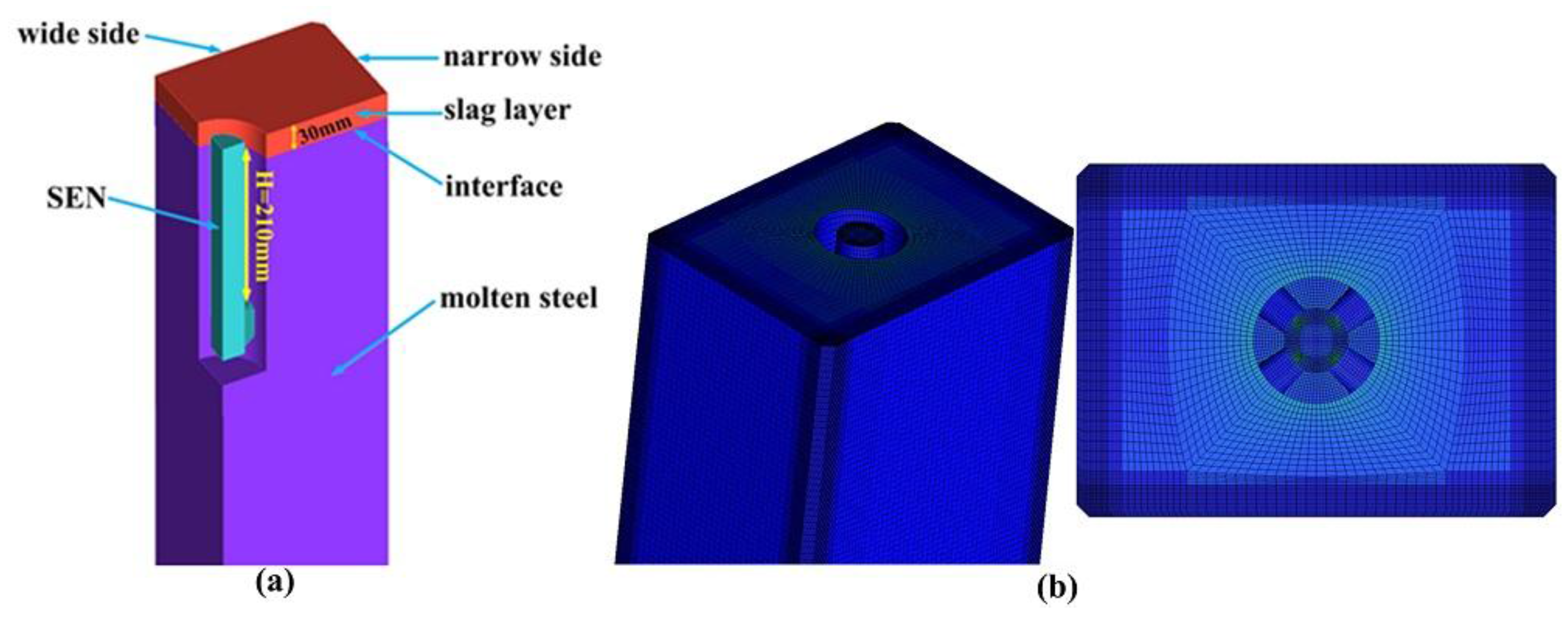
3.2. Model Building
3.3. Initial and Boundary Conditions
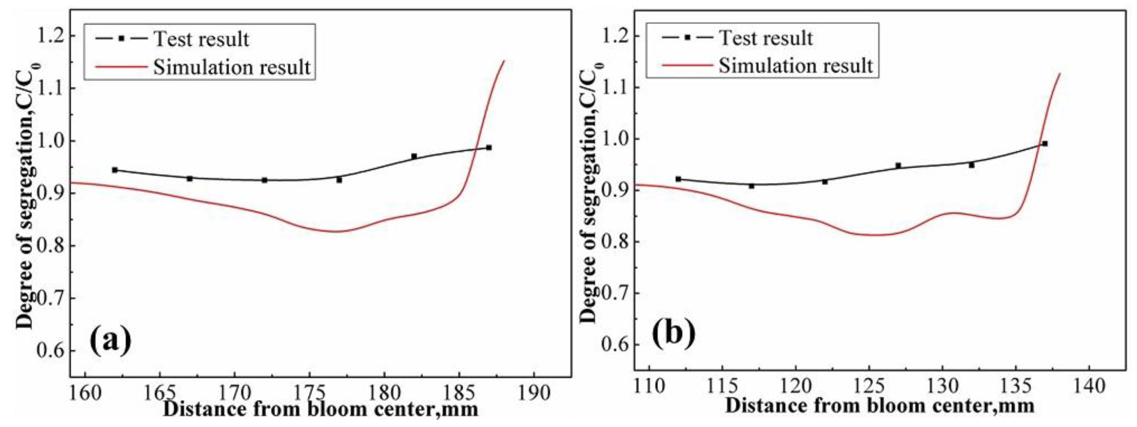
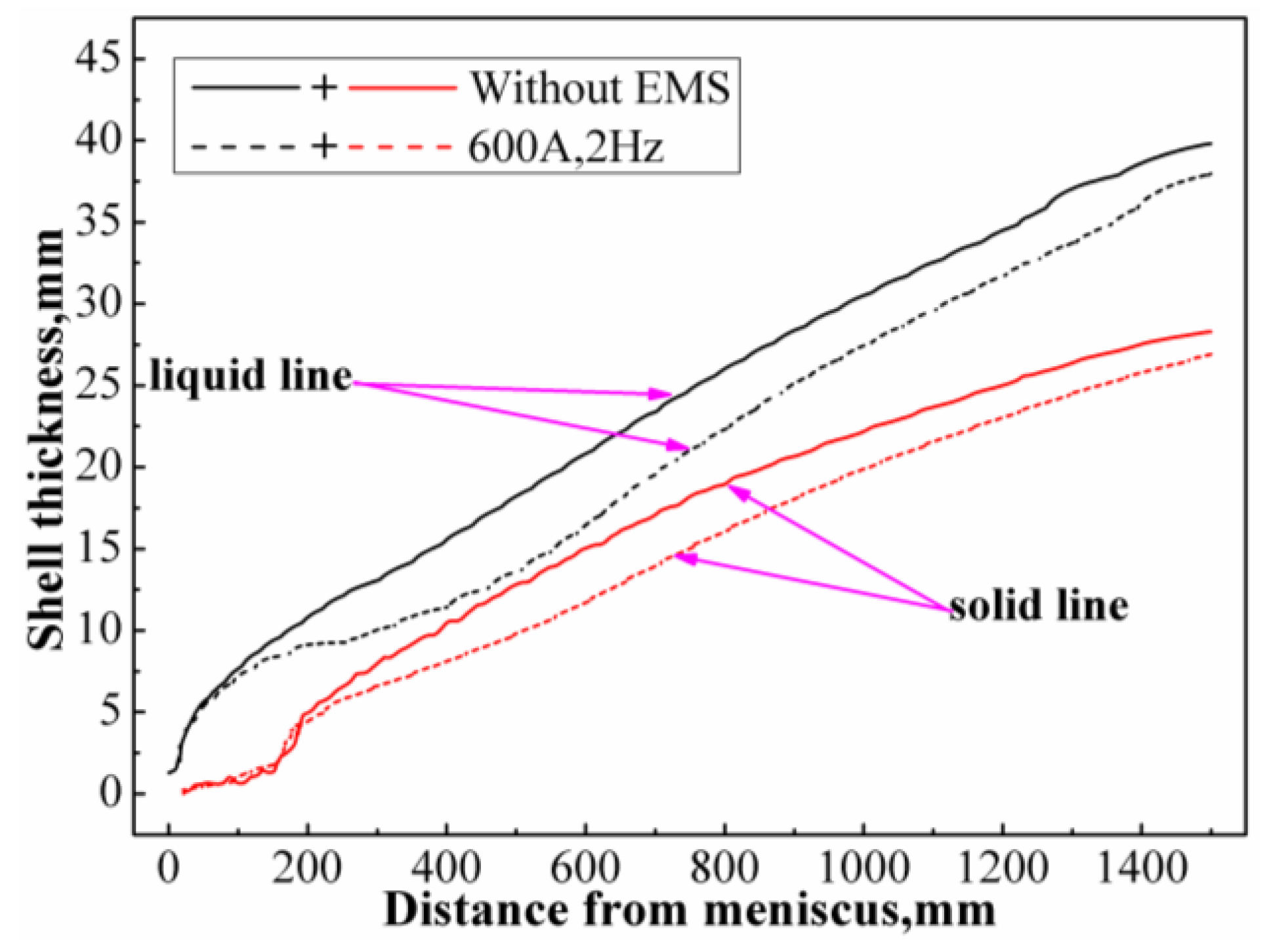
3.4. Verification of Solute Transport
4. Results and Discussion
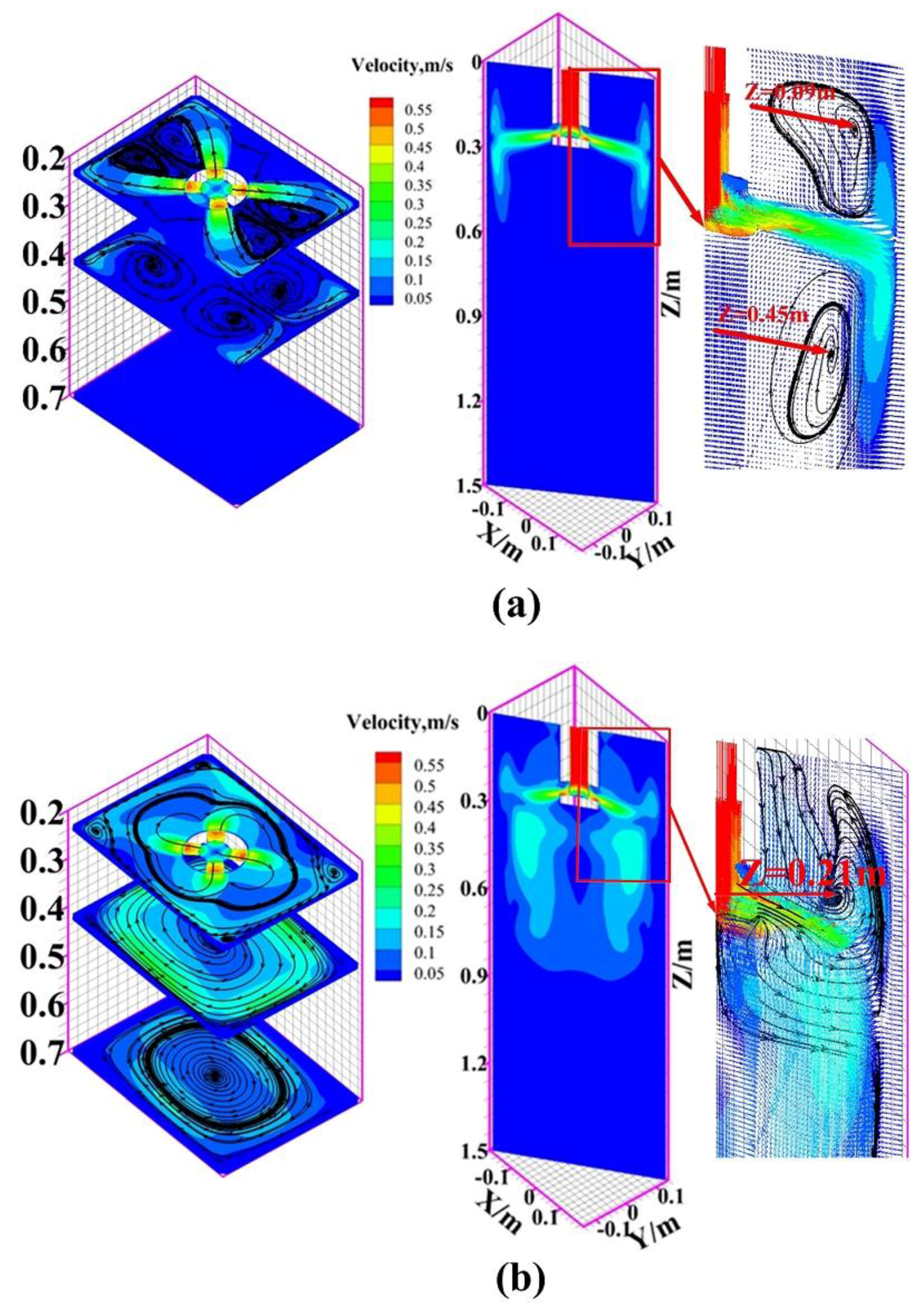
4.1. Metallurgical Effects of M-EMS
4.1.1. Flow Field
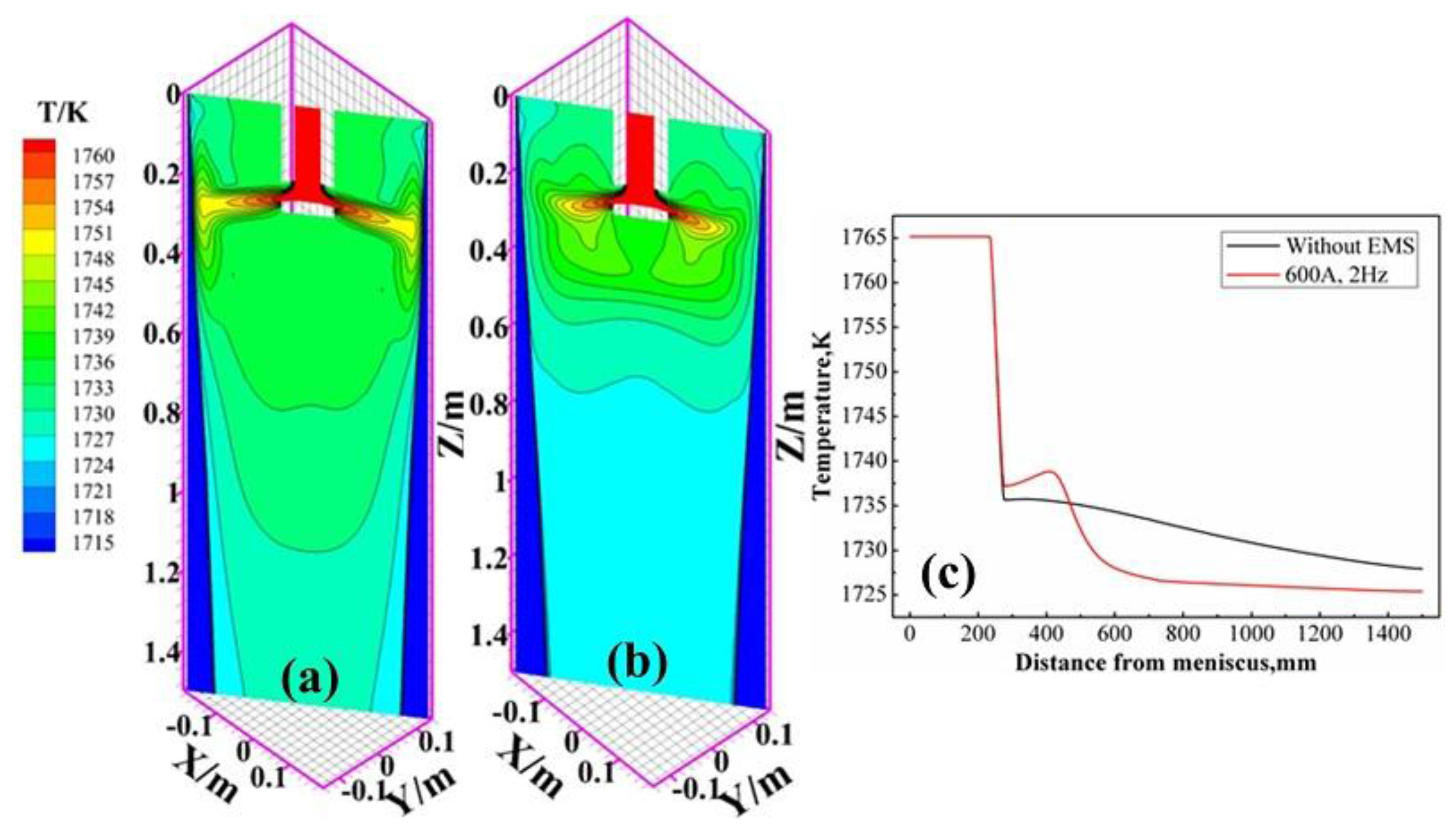
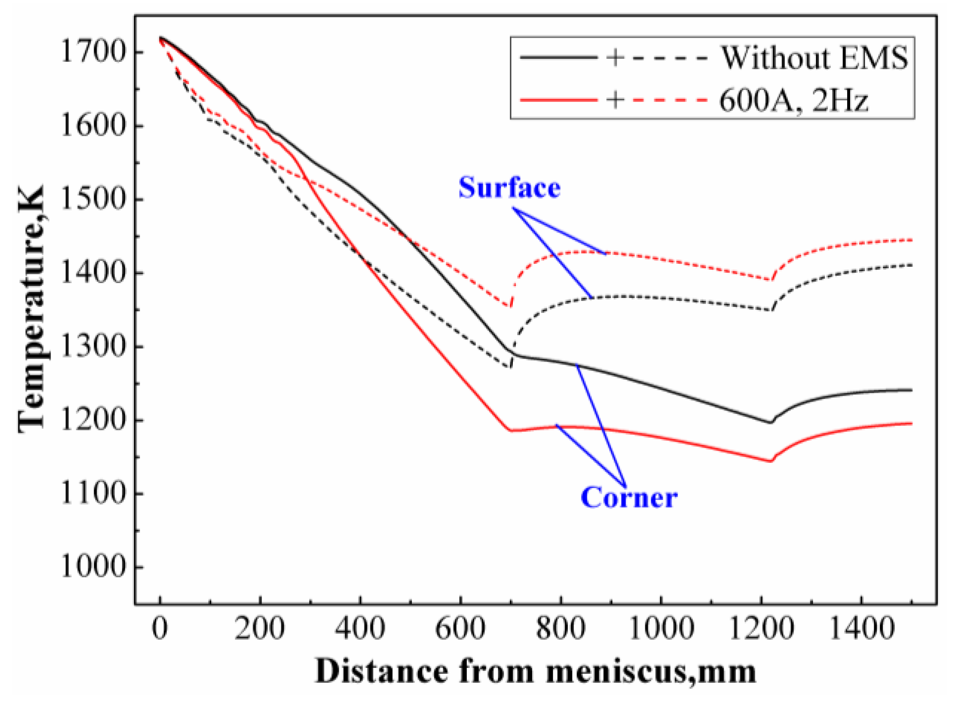
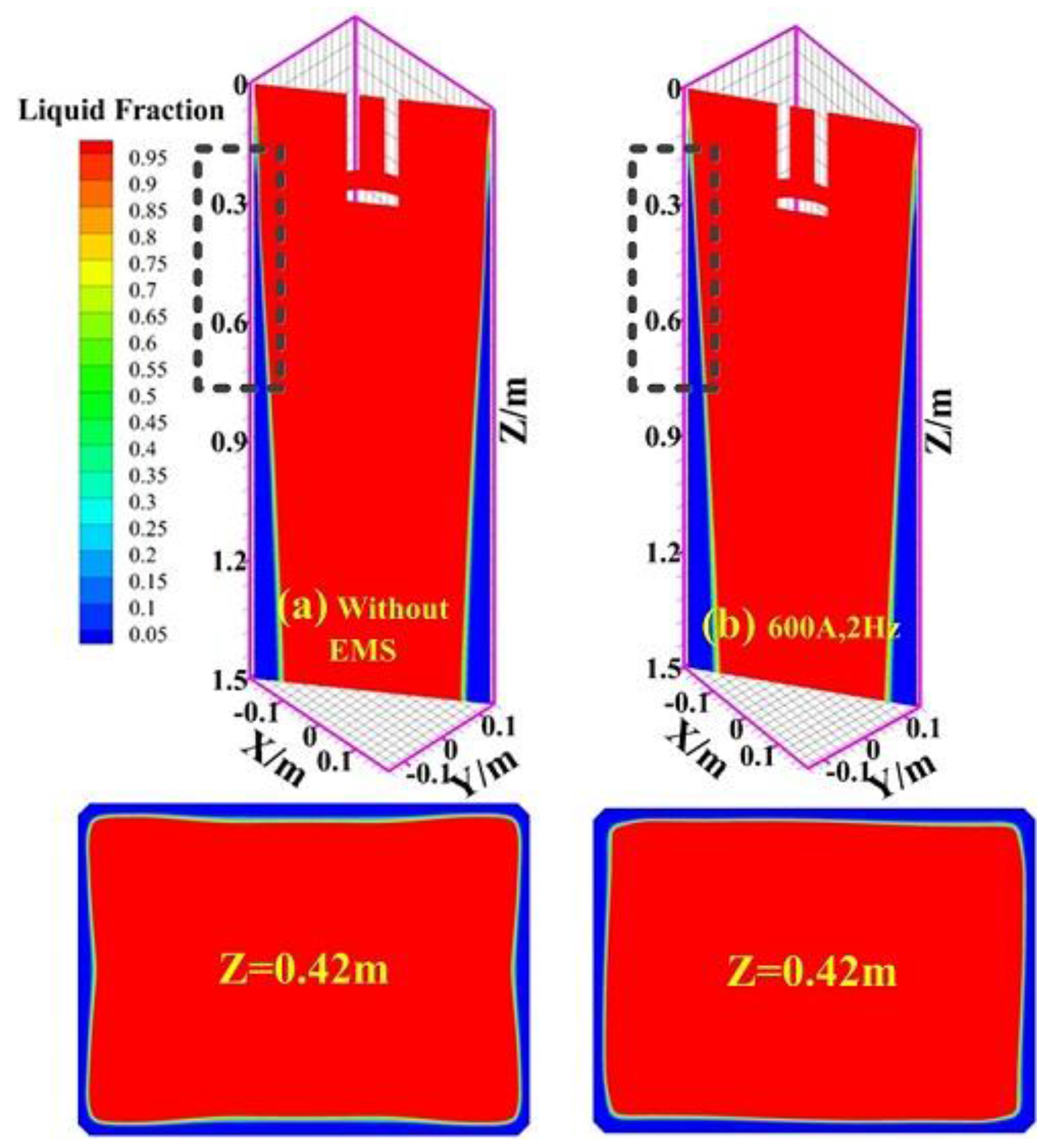
4.1.2. Heat Transfer and Solidification
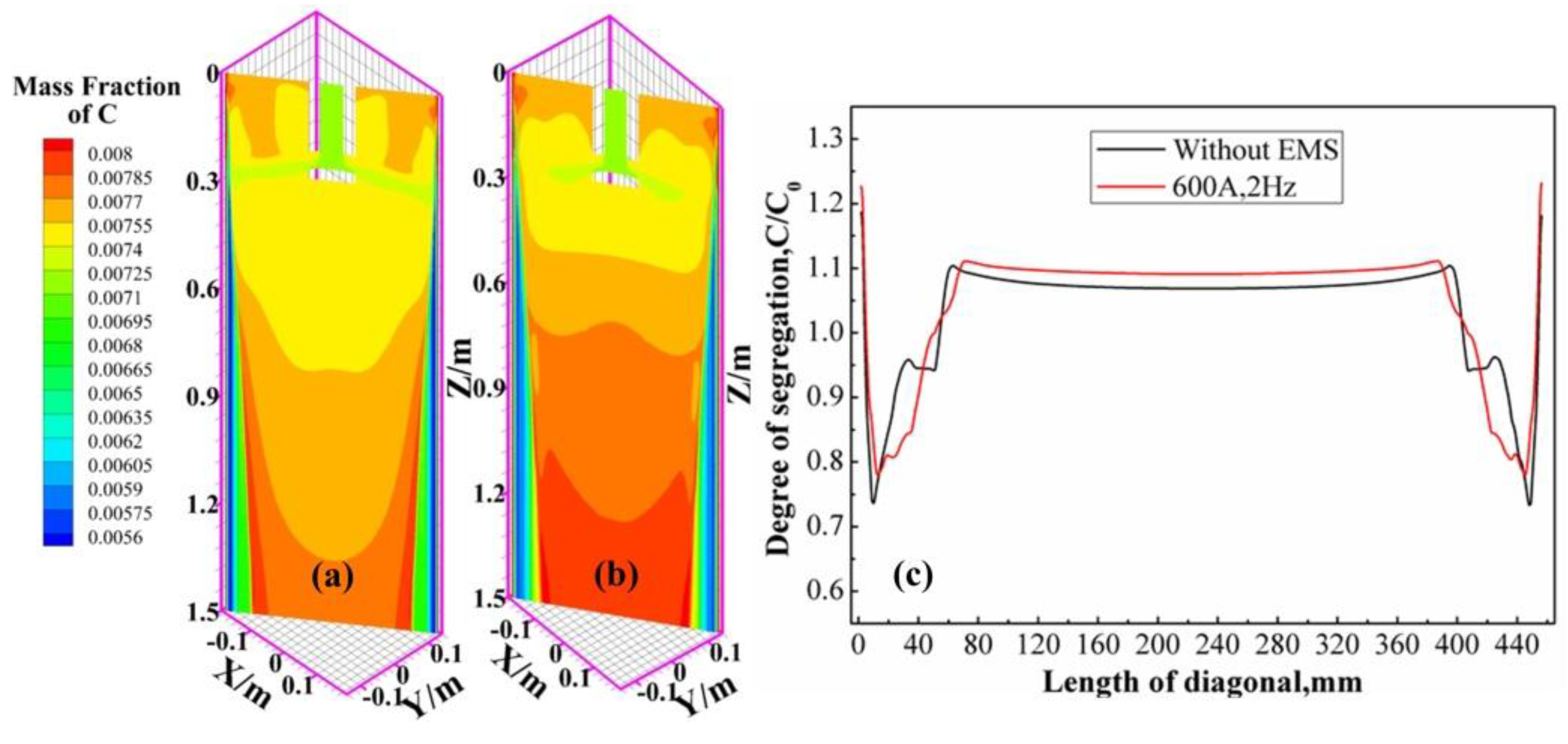
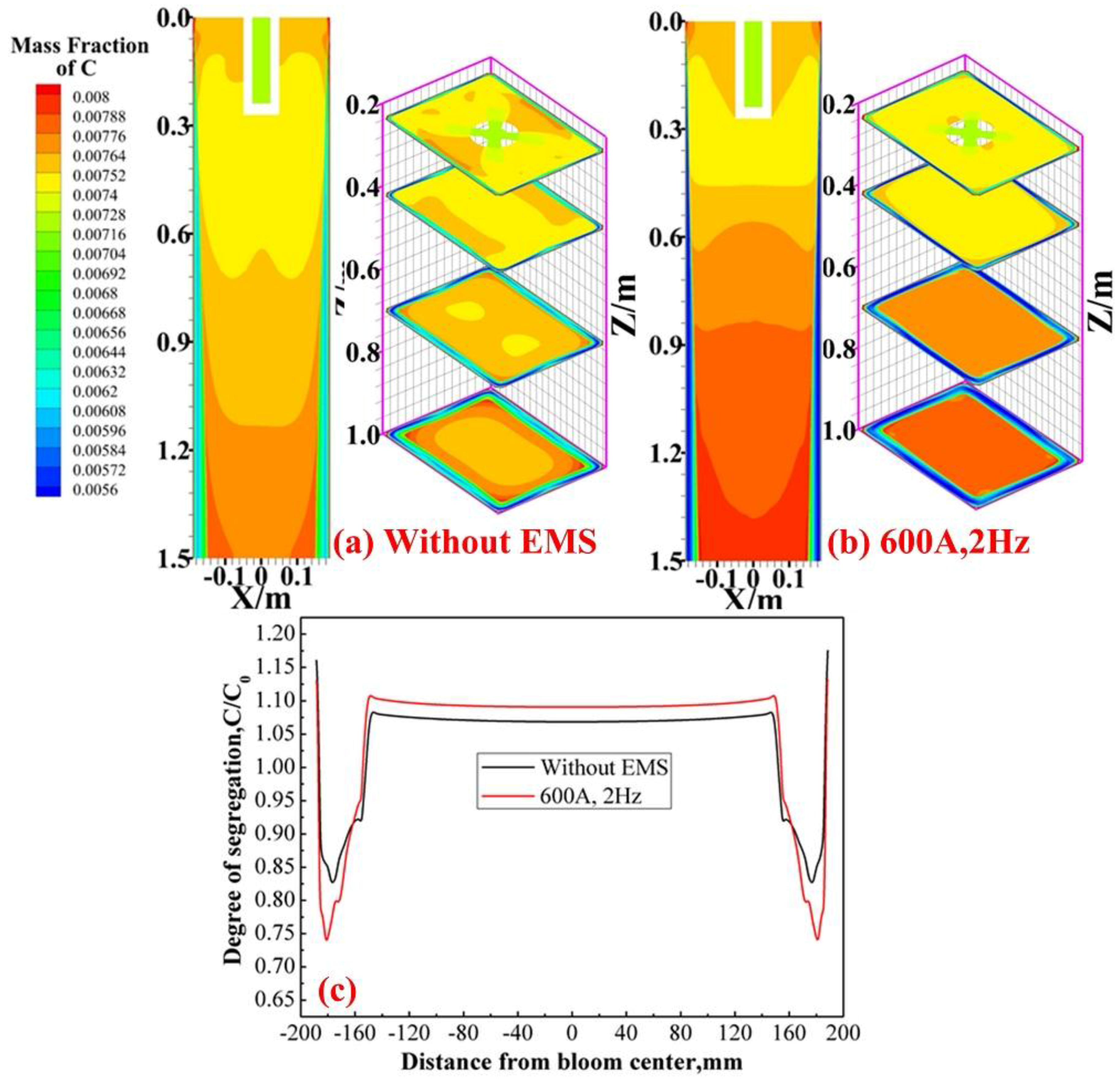
4.1.3. Solute Transport
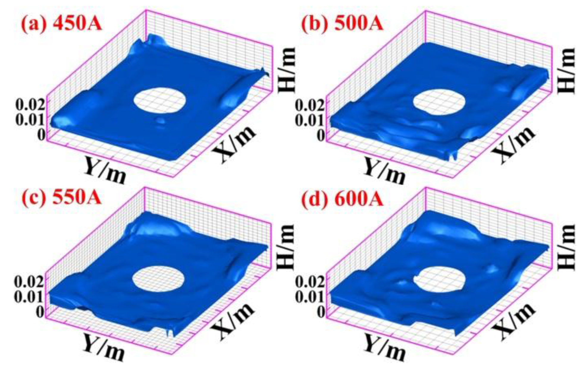
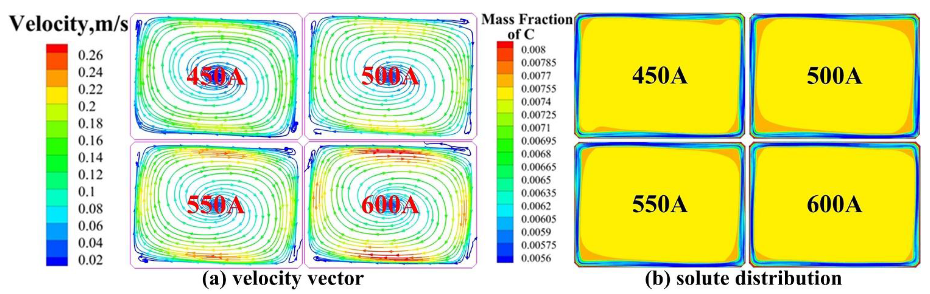
4.2. Effect of Current Intensity
5. Conclusions
- (1)
- The basically consistent variation tendency of the segregation profiles of solute element C in the region of the initial solidified shell with a thickness of 30 mm at both the wide and narrow sides can be observed between the simulated and measured results.
- (2)
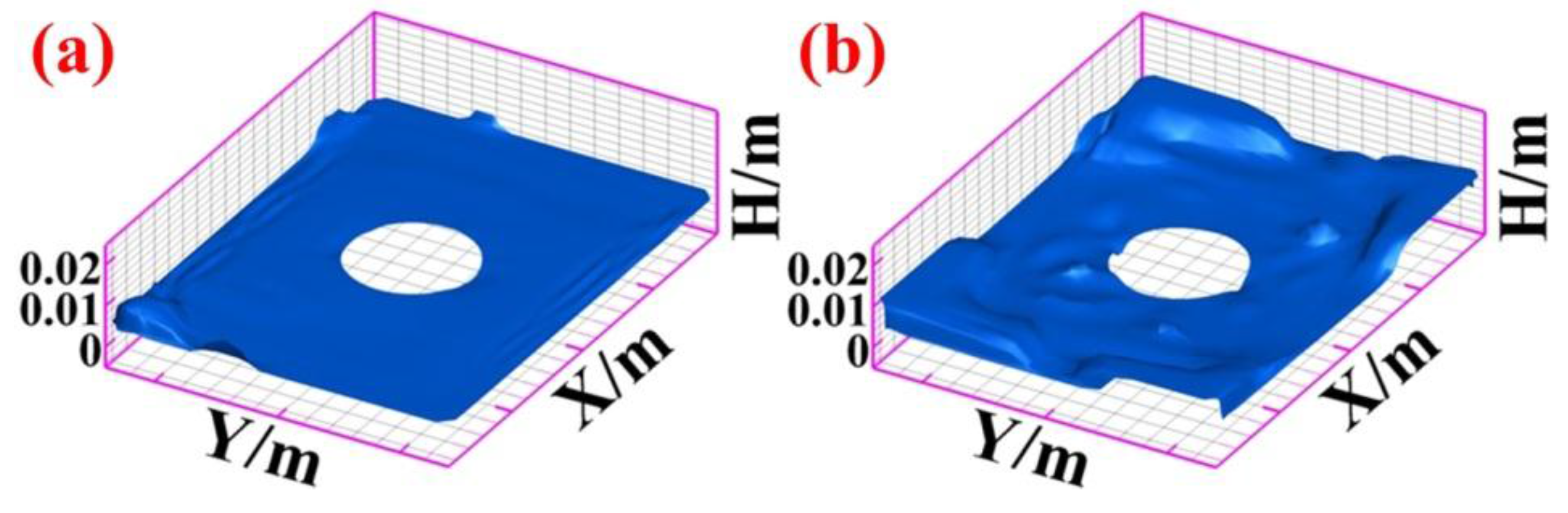
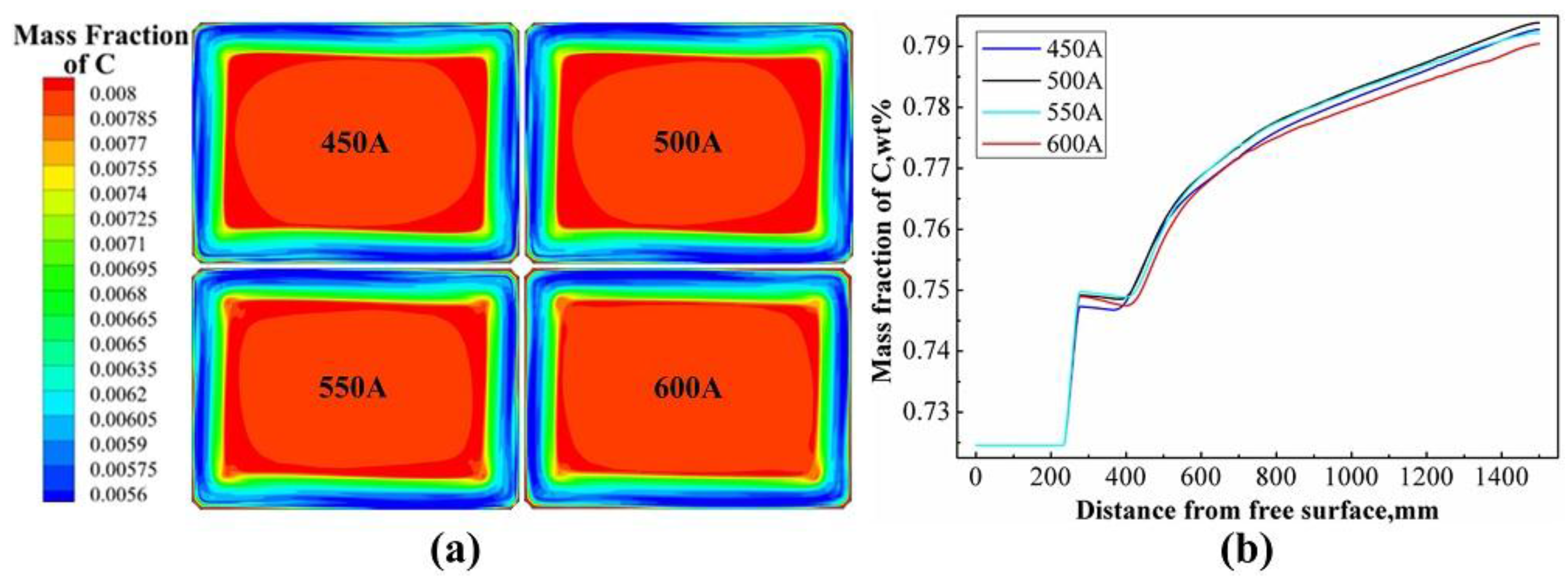
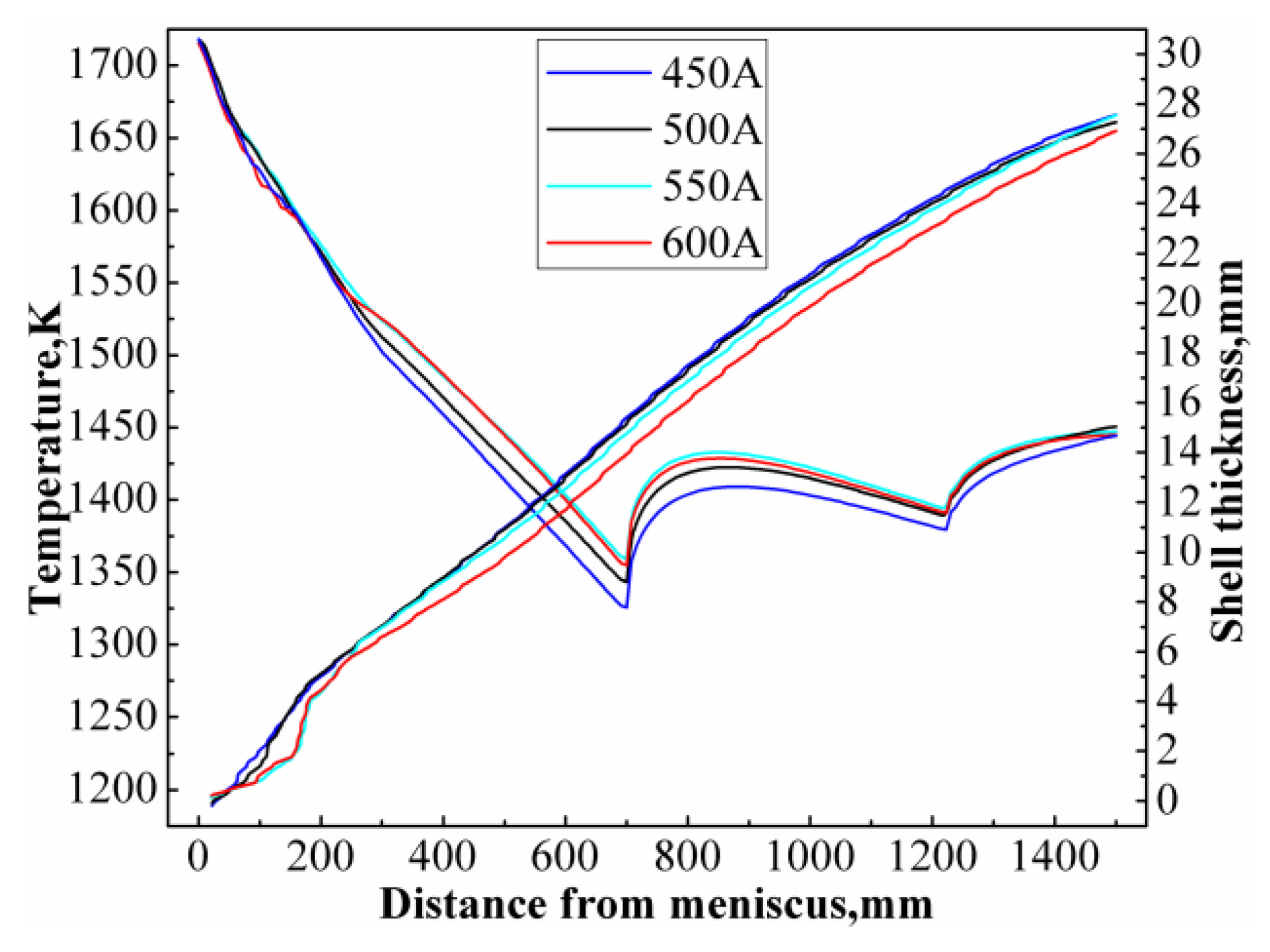
- Compared with the case without EMS, the bloom mold loaded with EMS is beneficial to the elimination of steel superheat, reduces the breadth of the mushy zone, and aggravates the level fluctuation from 4.5 mm to 6.2 mm. The distribution of temperature, solute, and solidified shell is more uniform in the EMS effective zone, the highest degree of negative segregation at the mold corner decreases from 0.78 to 0.74, but increases from 0.84 to 0.738 at the narrow and wide sides. The mass fraction of solute element C at the computational outlet increases from 0.7743% to 0.7904%. The EMS mold is not beneficial to the improvement of centerline segregation for big bloom casting.
- (3)
- With the increase of EMS current intensity (from 450 A to 600 A), the stirring effect and tangential velocity at the solidification front around the center of the wide and narrow sides increases, the level fluctuation is aggravated from 5.3 mm to 6.2 mm, the surface temperature in the EMS effective zone, the uniformity degree of temperature, and the solute distribution in the molten steel all increase as well, while the growth velocity of the solidifying shell thickness in the EMS effective zone decreases. The mass fraction of solute element C at the center of the computational outlets (z = 1.5 m) decreases from 0.7925% to 0.7904%. The M-EMS with a current intensity of 600 A is more suitable for big bloom castings.
- (4)
- The model has great application potential for a qualitative study of multi-physical phenomena in the bloom mold coupled with EMS, especially for the solute transport and solidification process coupled with turbulent flow. However, the present model would apply only to part of the caster, particularly the turbulent flow zone. To enhance the inner quality of the final products, the heat transfer and solute transport behavior below the computational domain need further investigation, especially for efficient ways to alleviate central segregation.
Acknowledgments
Author Contributions
Conflicts of Interest
References
- Wu, H.J.; Wei, N.; Bao, Y.P.; Wang, G.X.; Xiao, C.P.; Liu, J.J. Effect of M-EMS on the solidification structure of a steel billet. Int. J. Miner. Metall. Mater. 2011, 18, 159–164. [Google Scholar] [CrossRef]
- Sun, T.; Yue, F.; Wu, H.J.; Guo, C.; Li, Y.; Ma, Z.C. Solidification structure of continuous casting large round billets under mold electromagnetic stirring. J. Iron Steel Res. Int. 2016, 23, 329–337. [Google Scholar] [CrossRef]
- Jiang, D.B.; Zhu, M.Y. Solidification Structure and Macrosegregation of Billet Continuous Casting Process with Dual Electromagnetic Stirrings in Mold and Final Stage of Solidification: A Numerical Study. Metall. Mater. Trans. B. 2016, 47, 3446–3458. [Google Scholar] [CrossRef]
- Geng, X.; Li, X.; Liu, F.B.; Jiang, Z.H. Optimisation of electromagnetic field and flow field in round billet continuous casting mould with electromagnetic stirring. Ironmak. Steelmak. 2015, 42, 675–682. [Google Scholar] [CrossRef]
- Yu, H.Q.; Zhu, M.Y. 3-D Numerical simulation of flow field and temperature field in a round billet continuous casting mold with electromagnetic stirring. Acta Metal. Sin. 2008, 44, 1465. [Google Scholar]
- Liu, H.P.; Xu, M.G.; Qiu, S.T.; Zhang, H. Numerical simulation of fluid flow in a round bloom mold with in-mold rotary electromagnetic stirring. Metall. Mater. Trans. B 2012, 43, 1657–1675. [Google Scholar] [CrossRef]
- Singh, R.; Thomas, B.G.; Vanka, S.P. Large eddy simulations of double-ruler electromagnetic field effect on transient flow during continuous casting. Metall. Mater. Trans. B 2014, 45, 1098–1115. [Google Scholar] [CrossRef]
- Singh, R.; Thomas, B.G.; Vanka, S.P. Effects of a magnetic field on turbulent flow in the mold region of a steel caster. Metall. Mater. Trans. B 2013, 44, 1201–1221. [Google Scholar] [CrossRef]
- Timmel, K.; Eckert, S.; Gerbeth, G. Experimental investigation of the flow in a continuous-casting mold under the influence of a transverse, direct current magnetic field. Metall. Mater. Trans. B 2011, 42, 68–80. [Google Scholar] [CrossRef]
- Yang, Z.G.; Wang, B.; Zhang, X.F.; Wang, Y.T.; Dong, H.B. Effect of electromagnetic stirring on molten steel flow and solidification in bloom mold. J. Iron Steel Res. Int. 2014, 21, 1095–1103. [Google Scholar] [CrossRef]
- Ren, B.Z.; Chen, D.F.; Wang, H.D.; Long, M.J.; Han, Z.W. Numerical analysis of coupled turbulent flow and macroscopic solidification in a round bloom continuous casting mold with electromagnetic stirring. Steel Res. Int. 2015, 86, 1104–1115. [Google Scholar] [CrossRef]
- Tian, X.Y.; Zou, F.; Li, B.W.; He, J.C. Numerical analysis of coupled fluid flow, heat transfer and macroscopic solidification in the thin slab funnel shape mold with a new type EMBr. Metall. Mater. Trans. B 2010, 41, 112–120. [Google Scholar] [CrossRef]
- Ren, B.Z.; Chen, D.F.; Wang, H.D.; Long, M.J.; Han, Z.W. Numerical simulation of fluid flow and solidification in bloom continuous casting mould with electromagnetic stirring. Ironmak. Steelmak. 2015, 42, 401–408. [Google Scholar] [CrossRef]
- Sun, H.B.; Zhang, J.Q. Effect of feeding modes of molten steel on the mould metallurgical behavior for round bloom casting. ISIJ Int. 2011, 51, 1657–1663. [Google Scholar] [CrossRef]
- Aboutalebi, M.R.; Hasan, M.; Guthrie, R.I.L. Coupled turbulent flow, heat, and solute transport in continuous casting processes. Metal. Mater. Trans. B. 1995, 26, 731–744. [Google Scholar] [CrossRef]
- Yang, H.L.; Zhao, L.G.; Zhang, X.Z.; Deng, K.W.; Li, W.C.; Gan, Y. Mathematical simulation on coupled flow, heat, and solute transport in slab continuous casting process. Metal. Mater. Trans. B 1998, 29, 1345–1356. [Google Scholar] [CrossRef]
- Lei, H.; Zhang, H.W.; He, J.C. Flow, solidification, and solute transport in a continuous casting mold with electromagnetic brake. Chem. Eng. Technol. 2009, 32, 991–1002. [Google Scholar] [CrossRef]
- Kang, K.G.; Ryou, H.S.; Hur, N.K. Coupled turbulent flow, heat, and solute transport in continuous casting processes with an electromagnetic brake. Numer. Heat Transf. Part A 2005, 48, 461–481. [Google Scholar] [CrossRef]
- Sun, H.B.; Zhang, J.Q. Macrosegregation improvement by swirling flow nozzle for bloom continuous castings. Metal. Mater. Trans. B. 2014, 45, 936–946. [Google Scholar] [CrossRef]
- Asai, S.; Nishio, N.; Muchi, I. Theoretical analysis and model experiments on electromagnetically driven flow in continuous casting. ISIJ Int. 1982, 22, 126–133. [Google Scholar] [CrossRef]
- Jones, W.P.; Launder, B.E. The calculation of low-Reynolds-number phenomena with a two-equation model of turbulence. Int. J. Heat Mass Trans. 1973, 16, 1119–1130. [Google Scholar] [CrossRef]
- Lam, C.K.G.; Bremhorst, K. A modified form of the k-ε model for predicting wall turbulence. ASME Trans. J. Fluids Eng. 1981, 103, 456–460. [Google Scholar] [CrossRef]
- Poirier, D.R. Permeability of flow of interdentritic liquid in columnar-dendritic alloys. Metal. Mater. Trans. B 1987, 18, 245–255. [Google Scholar] [CrossRef]
- Li, W.S.; Shen, B.Z.; Shen, H.F.; Liu, B.C. Modelling of macrosegregation in steel ingots: Benchmark validation and industrial application. IOP Conf. Ser. Mater. Sci. Eng. 2012, 33, 1–8. [Google Scholar] [CrossRef]
- Hrenya, C.M.; Bolio, E.J.; Chakrabarti, D.; Sinclair, J.L. Comparison of low Reynolds number k-ε turbulence models in predicting fully developed pipe flow. Chem. Eng. Sci. 1995, 50, 1923–1941. [Google Scholar] [CrossRef]
- Spitzer, K.H.; Dubke, M.; Schwerdtfeger, K. Rotational electromagnetic stirring in continuous casting of round strands. Metall. Mater. Trans. B 1986, 17, 119–131. [Google Scholar] [CrossRef]
- Deng, A.Y.; Xu, L.; Wang, E.G.; He, J.C. Numerical analysis of fluctuation behavior of steel/slag interface in continuous casting mold with static magnetic field. J. Iron Steel Res. Int. 2014, 21, 809–816. [Google Scholar] [CrossRef]
- Zhao, Z.F.; Ni, H.W.; Zhang, H.; Chen, G.Y.; Yi, W.; Hong, J. Technology and process optimisation of bloom casting of ultrahigh speed rail steel. Ironmak. Steelmak. 2014, 41, 539–546. [Google Scholar] [CrossRef]
- Lai, K.Y.M.; Salcudean, M.; Tanaka, S.; Guthrie, R.I.L. Mathematical modeling of flows in large tundish systems in steelmaking. Metall. Mater. Trans. B 1986, 17, 449–459. [Google Scholar] [CrossRef]
- Alizadeh, M.; Jahromi, A.J.; Abouali, O. A new semi-analytical model for prediction of the strand surface temperature in the continuous casting of steel in the mold region. ISIJ Int. 2008, 48, 161–169. [Google Scholar] [CrossRef]
- Yu, H.Q.; Zhu, M.Y. Influence of electromagnetic stirring on transport phenomena in round billet continuous casting mould and macrostructure of high carbon steel billet. Ironmak. Steelmak. 2012, 39, 574–584. [Google Scholar] [CrossRef]
- Zeng, J.; Chen, W.; Wang, Q.; Wang, G. Improving inner quality in continuous casting rectangular billets: Comparison between mechanical soft reduction and final electromagnetic stirring. Trans. Indian Inst. Metals 2016, 69, 1–10. [Google Scholar] [CrossRef]


| Chemical Composition | C | Si | Mn | P | S | Cr | Mo | Ni | Cu |
|---|---|---|---|---|---|---|---|---|---|
| Mass% | 0.73 | 0.25 | 1.2 | ≤0.02 | ≤0.02 | ≤0.15 | ≤0.02 | ≤0.10 | ≤0.15 |
| Parameters | Value |
|---|---|
| Cross section of bloom, mm2 | 380 × 280 |
| Casting speed, m/min | 0.63 |
| Casting temperature, K | 1765 |
| Nozzle adaption | Figure 2 |
| Calculation length, mm | 1500 |
| Running current of M-EMS, A | 450–600 |
| Running frequency of M-EMS, Hz | 2.0 |
| EMS center(distance from meniscus), mm | 420 |
| Height of EMS, mm | 480 |
| Water quantity in mold, L/min | 2600 |
| Parameters | Value |
|---|---|
| Operation density, kg/m3 | 7020 |
| Latent heat, J/kg | 272,000 |
| Specific heat of liquid, J/(kg·K) | 810 |
| Specific heat of solid, J/(kg·K) | 682 |
| Electric conductivity, S/m | 7.14 × 10⁵ |
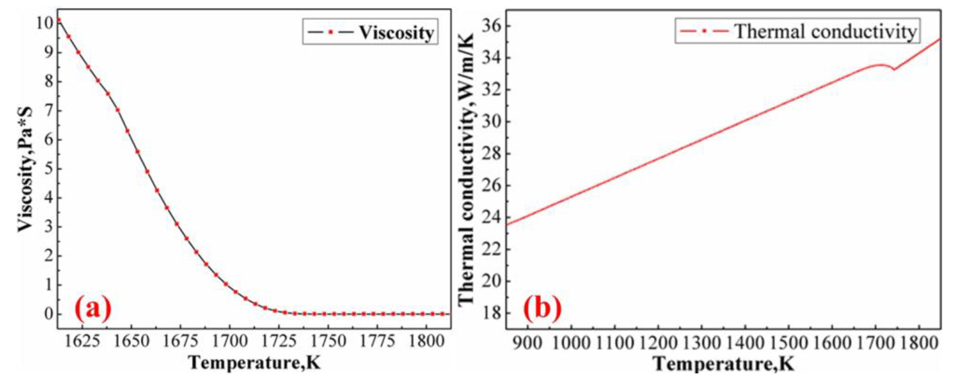
| Viscosity, Pa·s | Figure 3a |
| Thermal conductivity, W/(m·K) | Figure 3b |
| Diffusion coefficient of liquid, cm2/s | |
| Diffusion coefficient of solid, cm2/s | |
| Equilibrium partition coefficient | 0.4 |
| Slope of liquidus line | 78 |
© 2017 by the authors. Licensee MDPI, Basel, Switzerland. This article is an open access article distributed under the terms and conditions of the Creative Commons Attribution (CC BY) license ( http://creativecommons.org/licenses/by/4.0/).
Share and Cite
Fang, Q.; Ni, H.; Wang, B.; Zhang, H.; Ye, F. Effects of EMS Induced Flow on Solidification and Solute Transport in Bloom Mold. Metals 2017, 7, 72. https://doi.org/10.3390/met7030072
Fang Q, Ni H, Wang B, Zhang H, Ye F. Effects of EMS Induced Flow on Solidification and Solute Transport in Bloom Mold. Metals. 2017; 7(3):72. https://doi.org/10.3390/met7030072
Chicago/Turabian StyleFang, Qing, Hongwei Ni, Bao Wang, Hua Zhang, and Fei Ye. 2017. "Effects of EMS Induced Flow on Solidification and Solute Transport in Bloom Mold" Metals 7, no. 3: 72. https://doi.org/10.3390/met7030072