An Efficient Fluid-Dynamic Analysis to Improve Industrial Quenching Systems

Abstract

This paper addresses the problem of understanding the relationship between fluid flow and heat transfer in industrial quenching systems. It also presents an efficient analysis to design or optimize long standing quenching tanks to increase productivity. The study case is automotive leaf springs quenched in an oil-tank agitated with submerged jets. This analysis combined an efficient numerical prediction of the detailed isothermal flow field in the whole tank with the thermal characterization of steel probes in plant and laboratory during quenching. These measurements were used to determine the heat flow by solving the inverse heat conduction problem. Differences between laboratory and plant heat flux results were attributed to the difference in surface area size between samples. A proposed correlation between isothermal wall shear stress and heat flux at the surface of the steel component, based on the Reynolds-Colburn analogy, provided the connection between thermal characterization and computed isothermal fluid flow. The present approach allowed the identification of the potential benefits of changes in the tank design and the evaluation of operating conditions while using a much shorter computing time and storage memory than full-domain fluid flow calculations.

1. Introduction

The generation of a quantitative understanding of fluid dynamics and heat transfer during quench tank production is a research area that offers wide space for technical contributions. Many of commercially important steels and aluminum alloys are heat-treated to achieve the target hardness and tensile strength. This treatment consists of heating the metallic pieces to their dissolution temperature and then quenching them by fast cooling. Water, aqueous polymer, oil, molten salt or gas is generally used as a quenching medium, and the choice depends on the alloy chemical composition and the desired mechanical properties of the product. Commercial alloys have been properly formulated for suitable quenching to reach specific property values. However, long-standing production tanks introduce a major challenge: controlling agitation, its intensity and uniformity. Agitation plays a key role in determining the rate of heat transfer from the workpieces to the quenching medium. When a hot solid piece is immersed into the liquid, boiling occurs. First, a vapor film develops over the surface, and the rate of heat transfer is controlled by the isolating properties of this stable vapor film. Once the surface cools to reach the so-called Leidenfrost temperature, the vapor film collapses, and the liquid directly contacts the solid surface, generating a swarm of bubbles detaching from the surface. This leads to a fast increase in the heat flux to reach a maximum value, the so-called critical heat flux. During cooling, solid-phase transformations occur in the metal that create one or more new phases with required mechanical properties. For example, austenite (a solid solution of carbon in gamma iron with face-centered cubic lattice) is transformed into hard phase martensite (a supersaturated solid solution of carbon in alpha iron with body-centered tetragonal lattice) when steel is quenched from austenitization temperature to a temperature below M_s (martensite start temperature). The specific volume of martensite is ~3.5% higher than the corresponding value of austenite, which may lead to an adverse effect during non-uniform cooling. The internal stresses in the solid that are generated from this phase transformation combine with stresses promoted by thermal gradients, and the result may produce disastrous consequences in terms of distortion and/or crack formation in the product. Furthermore, spot areas where the stable vapor film remained for a long time would probably lead to low spotty hardness as result of an insufficient cooling rate to generate the desired solid-phase transformation.

Industrial quenching practice has largely remained on a semi-empirical basis because there is a minimal quantitative understanding of the quenching process itself in many heat treating shops [1]. Heat treating engineers and equipment suppliers struggle to find design and operating solutions without any industry-wide guidelines for quench system design, except for some company specifications. Although it is well known that fluid flow varies greatly as a function of position within industrial tanks, fluid velocity distribution monitoring is rarely found in production quench systems. An important reason for this is that properly designed flow devices with sufficient sensitivity and ruggedness for use in a heat treating shop are not fully commercially available, as mentioned in [2]. This reference presents a useful compilation of the existing flow process sensors and methods.

The state of the art in the application of fundamental knowledge to understand the complex quenching phenomena is better appreciated from a review of a number of publications presenting mathematical models of this process.

Table 1. Evolution of predictive power of mathematical models developed for metal quenching.

Author (s), Year	CFD	Heat Conduction	Solid-Phase Transformation	Residual Stress and Distortion
Totten et al., 1993	Isothermal fluid flow	-	-	-
Garwood et al., 1992		-	-	-
Halva and Volny, 1993		-	-	-
Bogh, 1994		-	-	-
Kernazhitskiy, 2003		-	-	-
Kumar et al., 2007		-	-	-
R.-Bineli et al., 2010	Non-isothermal but no-boiling flow	Non-isothermal solid	-	-
Krause et al., 2010	Mixed fluids	Isothermal and non-isothermal solids	-	-
Srinivasan et al., 2010		Non-isothermal solid	-	-
Gao et al., 2011			yes	yes
Ricci et al., 2011	Computed interface, VOF		yes	-
El-Kosseifi, 2012	Computed interface, LS	Non-isothermal solid	-	-
Yang et al., 2013	Isothermal flow	-	-	-
Banka et al., 2013		Non-isothermal solid	yes	yes
Ko et al., 2013	Mixed fluids	Non-isothermal solid	-	Hardness prediction using Quenching Factor Analysis (QFA)
Kopun et al., 2014			-	-
Passarella et al., 2014			yes	yes

presents the evolution of the predictive power of mathematical models developed for metal quenching using a liquid. This is not a comprehensive list; its purpose is merely to offer a notion of the general trend in modeling according with the purpose of this work. The reader can find a complete and detailed review of the quench numerical models in [3]. Table 1 shows that from the early 1990s to the beginning of this 21st century, computational fluid dynamics (CFD) focused on isothermal fluid flow calculations. In these works [4,5,6,7,8,9], the Navier-Stokes and continuity equations were numerically solved together with turbulence equations under steady state conditions. The pioneering work of Totten et al. [4] showed that flow is not uniform in quenching tanks. Garwood et al. [5] validated their fluid flow calculations for an industrial tank using a laboratory physical model in which quantitative velocity measurements were carried out using Laser Doppler anemometry (LDA). Halva and Volný [6] computed isothermal fluid flow to examine the homogeneity of velocity distribution as a function of agitator placement. The effect of the location of spray eductors around a rack of aluminum panels on flow homogeneity was studied by Bogh [7]. Isothermal fluid flow simulations were computed by Kernanzhitskiy [8], who used these results combined with Taguchi partial factorial statistical analysis methodology to provide innovative design concepts for a new quenching system design. Kumar et al. [9] evaluated flow uniformity around automotive pinion gears during quenching. The success of fluid flow simulations was further boosted by more powerful and available computer facilities. In the present decade, new contributions appeared that solved, simultaneously with CFD equations, the transient heat conduction equation to determine the temperature evolution of a solid body within the computational domain [10,11,12,13,14,15,16,17,18]. References [13,14,18] also solved the corresponding solid-phase transformation kinetic equations, and in [13,18], the residual stress and deformation were additionally computed. Reference [10] presented simulations of two systems of agitation in a quench process. The authors assumed a non-isothermal fluid flow in contact with a solid with time-dependent temperature. However, boiling was not considered in their formulation. The heat transfer coefficient was computed from the temperature profile in a turbulent boundary layer. In this way, the authors could obtain a heat transfer coefficient that changed with both the position on a solid surface and time.

References [11,12,13,16,17,18] moved a step forward by simulating boiling heat transfer using the mixed fluids approach. This method considers two intermixed or interpenetrated fluids (vapor and liquid) with the space-dependent void fraction of every phase. Momentum, continuity and energy equations are written for each phase and solved simultaneously. The rates of exchange of mass, momentum and energy between phases are included as source terms in the corresponding equations and are calculated from empirical expressions. Therefore, this approach requires to define the corresponding empirical constants. Krause et al. [11] considered both isothermal and non-isothermal solid bodies. The numerical results obtained for the former case correspond to a steady-state boiling heat transfer for which there is a considerable number of reported works. Therefore, the authors validated their model against literature results. Srinivasan et al. [12] implemented their laminar flow model in the commercial code AVL-FIRE (the AVL-designed 3D CFD software package) to simulate the temperature evolution of a solid plate dipped at a given velocity in static water in a laboratory container. The quenching of an “S”-shaped part was reported in [13]. The authors computed the solid-fluid heat flux from a balance between the heat required to evaporate, quench and facilitate liquid convection according with the heat flux partitioning model, the so-called Rensselaer Polytechnic Institute (RPI) model of subcooled boiling, implemented in the Fluent code. They presented a computed heat transfer coefficient that changes with time and the position on the solid surface and the corresponding computed deformation and stress distribution of the part. A more fundamental CFD approach was presented in [14,15] in which multiphase boiling heat transfer was computed by considering a single fluid with space-dependent properties to calculate the interface position where the physical properties jump from liquid to gas values. Level set (LS), Volume of Fluid (VOF) and Phase Field are examples of methods in this category. The results from this approach provide a detailed picture of the actual boiling phenomena, such as the rates of nucleation, growth and detachment of bubbles. However, it demands considerable computational effort because the time and space steps for numerical integration should be very small. Isothermal flow calculations gained importance in [19,20]. Yang et al. [19] combined the CFD results with artificial neural network (ANN) analysis to determine an optimal design of water flow distribution in a quenching tank for large and complicated aluminum alloy workpieces. A relatively small number of fluid flow simulations provided enough data to the ANN algorithm to determine the optimal position of directional flow baffles and agitation speed. Reference [20] evaluated the effect of orientation of a hot ring with respect to the direction of a fluid flowing around it. Heat transfer was computed assuming a constant solid surface 100 °C above the fluid temperature. However, the authors computed the temperature evolution in the solid and its kinetics of solid-phase transformation and ring distortion.

The previous literature review indicates that predictions of solid-phase transformation kinetics and steel distortion and hardness depend on the knowledge of the rate of heat transfer during quenching. Typically, the heat transfer coefficient is used to establish a thermal boundary condition on the solid surface. However, available data of this coefficient are seldom related to the specific fluid dynamic conditions in industrial tanks and therefore simplifying assumptions are adopted for its determination. The present work proposes a correlation between isothermal wall shear stress and heat flux at the surface of a quenching steel component. This correlation is then used to evaluate more accurately the solutions proposed from the isothermal fluid-dynamic analysis during steel quenching in industrial tanks. In contrast to the commonly found full-domain calculations in which the momentum and mass equations are solved simultaneously in the whole domain, the present work shows fluid flow calculations that were efficiently carried out in “cascade downstream sequence”. This method allowed a high level of detail to be obtained in the flow field by using an order of magnitude fewer volume elements of fluid and a much shorter computation time compared with full-domain calculations. Therefore, it was possible to carry out multiple numerical simulations in a relatively short time to search for a new design that would improve the oil velocity around the leaf springs.

2. Materials and Methods

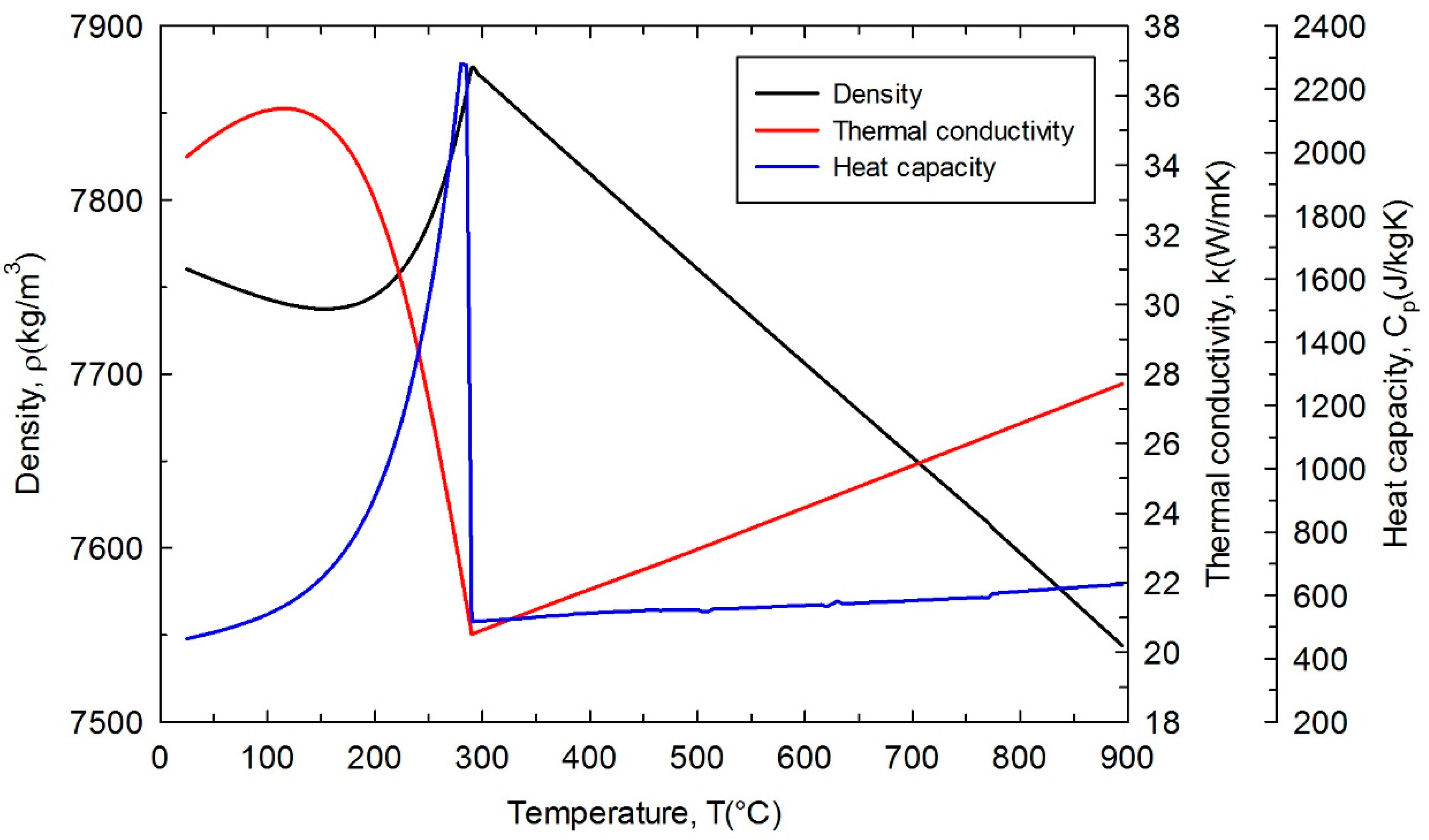
2.1. Materials Properties

Table 2. Chemical composition of DIN 51CrV4 steel employed.

Chemical Composition	C	Si	Mn	P	S	Cr	V	Sum of Others 1
Mass %	0.50	0.24	0.97	0.04	0.008	1.04	0.14	<0.281

¹ Analyzed impurity elements are: Cu (0.14), Ni, Mo, Al (0.07), N, O, Ti, and Nb. Balance is Fe.

shows the chemical composition of the leaf springs considered for this study and

Table 3. Thermophysical properties of materials. See Figure 1 for k, ρ and C_p of steel.

Material	kt (W/m·K)	ρ (kg/m3)	Cp (J/kg·K)	μ (mPa·s)	Tsat (°C)	Ms (°C)	M50 (°C)	M90 (°C)
Steel: 51CrV4	k(T)	ρ(T)	Cp(T)	-	-	288	251	166
Oil: FTR (Equiquench 770) Houghto-Quench®	-	827 at 60 °C	-	7.3 at 60 °C	290	-	-	-

presents the thermophysical properties of the steel and the quenching oil. Chemical composition was obtained from a spark optical emission spectrometry analysis. C, S, O and N were determined from combustion with infrared absorption detection analysis; O and N additionally required thermal conductivity analysis. Knowledge of the dependence of steel density, thermal conductivity and heat capacity with temperature is mandatory for a heat flow analysis. Figure 1 shows the corresponding property plots determined from JMatPro^® software data base (Version 9, Sente Software Ltd., Surrey Technology Center, Guildford, UK, 2016) using the chemical composition of steel and an austenitic grain size of ASTM 9. These property values were determined considering the cooling of austenite to form martensite. The leaf springs are quenched at rates of cooling that essentially produce only martensite throughout their whole cross section area. The table shows the density; viscosity; boiling point, T_sat; and temperatures for the start of martensite formation, M_s, and 50% and 90% of martensite formation, M₅₀ and M₉₀, respectively.

Figure 1 shows an abrupt change of properties at temperature of martensite start, M_s = 288 °C. Density decreases, while thermal conductivity and heat capacity increase. This later property includes the latent heat of solid-phase transformation from austenite to martensite.

The heat capacity of the transforming steel was computed from the following equation,

$$C_{\mathrm{p}}=\frac{\partial \left(x_{\mathrm{a}}{H}_{\mathrm{a}}+x_{\mathrm{m}}{H}_{\mathrm{m}}\right)}{\partial T},$$

(1)

where x is the mass fraction, H is the enthalpy per unit mass, and subscripts “a” and “m” refer austenite and martensite, respectively. Note that both quantities depend on temperature; the mass fraction depends on the kinetics of transformation, while enthalpy depends on the heat capacity of the corresponding phase.

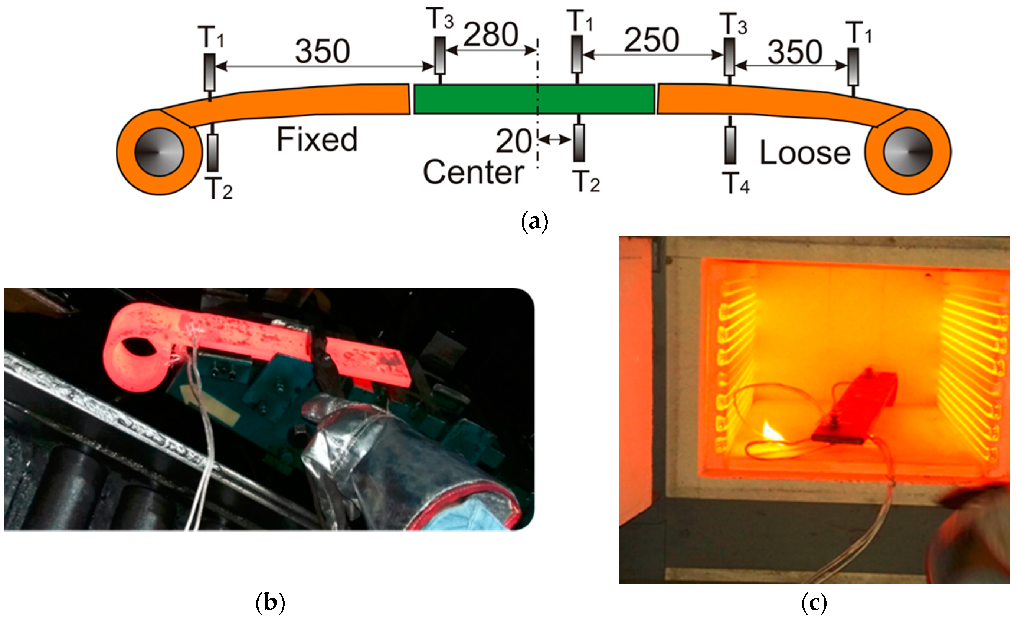
2.2. Plant Temperature Measurements

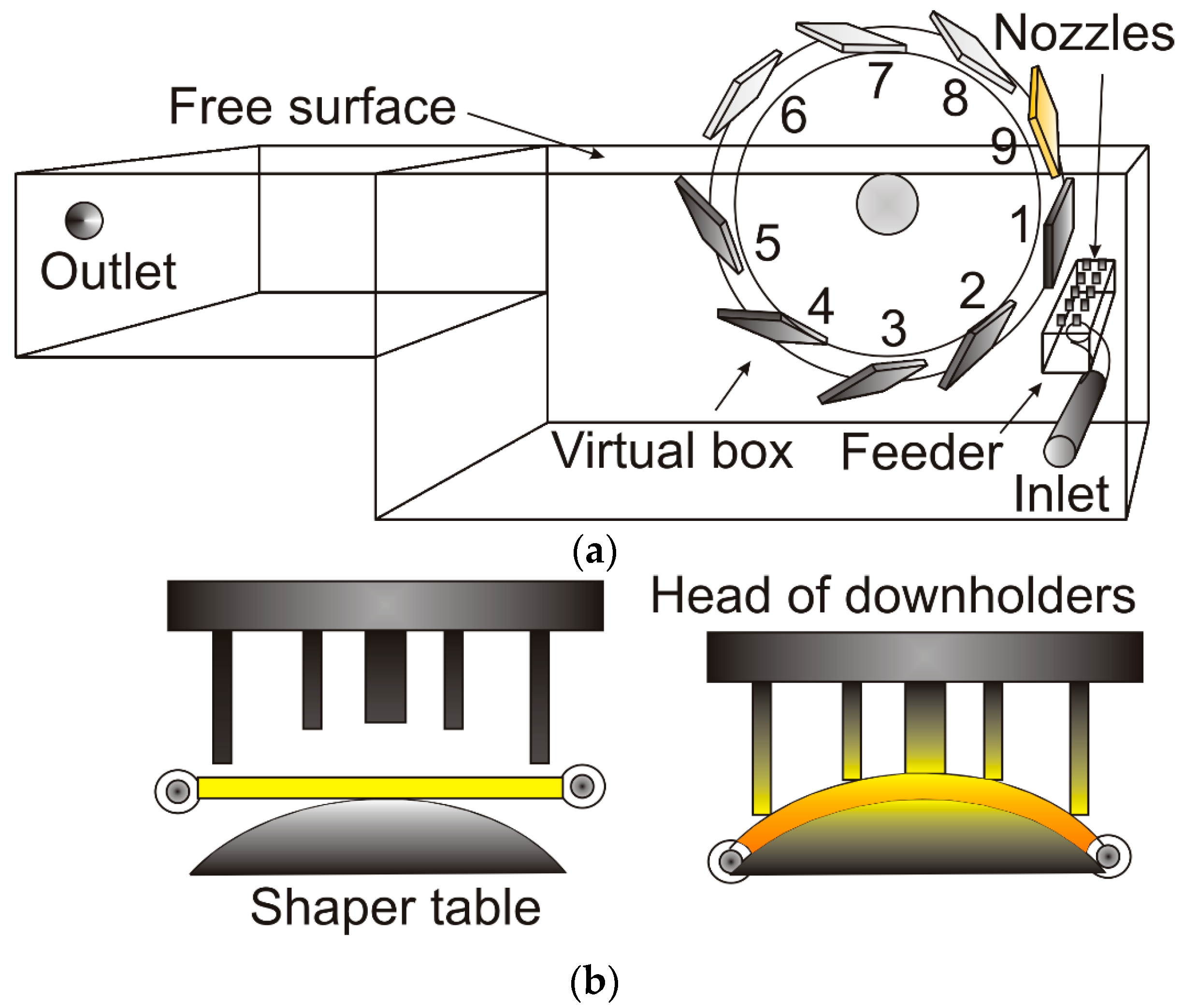
2.2.1. The Quenching System

The study case was an oil quenching tank with a carousel provided with tools to shape and hold steel leaf springs, 17 mm thick, 120 mm length and 75 mm wide, while they are immersed in the oil, as shown schematically in Figure 2a. In preparation for quenching, two preheated straight leaf springs are manually accommodated in a shaper table at position 9 of the carousel. A head of downholders then descends over the leaf springs, holding them against the shaper table, as shown in the drawings of Figure 2b. The carousel rotates and submerges the springs in the oil, stopping at position number 1. The operator charges another two leaf springs at position 9 and repeats the process. There are five carousel positions immersed in the oil; see numbers 1 to 5 in Figure 2a. When the leaf springs reach the sixth one, the head of downholders releases the shaped springs, and a robot arm takes them out to a transporting band. The dimensional specifications of the quenching system are given in

Table 4. Dimensional specifications of the quenching system.

Tank Component	Length (m)	Width (m)	Height (m)	Diameter (m)
Feeder, tube	-	-	-	0.197
Feeder, hexahedron	1.78	0.20	0.16	-
Nozzle	0.045	-	-	0.0254
Tank (main body)	2.96	2.11	2.74	-
Virtual box	0.22 (thickness)	1.46	0.57	-
Tank exit orifice	-	-	-	0.250

. A constant oil flowrate enters through the feeder tube and then flows through two rows of nozzles to generate immersed jets that feed the tank. The oil flows out from the tank to a cooling tower, which prevents it from overheating. When this tank increased the productivity of automotive leaf springs, an unacceptable distortion of the product was found.

Previous research work [21] presented some clues to determine the reason for this distortion. The objective of the present work was to develop an efficient fluid-dynamic analysis aimed to gain understanding of the cooling process of the leaf springs. This knowledge was used to analyze changes in the tank design to improve its fluid-dynamics and ultimately the rate of heat transfer from the steel leaves.

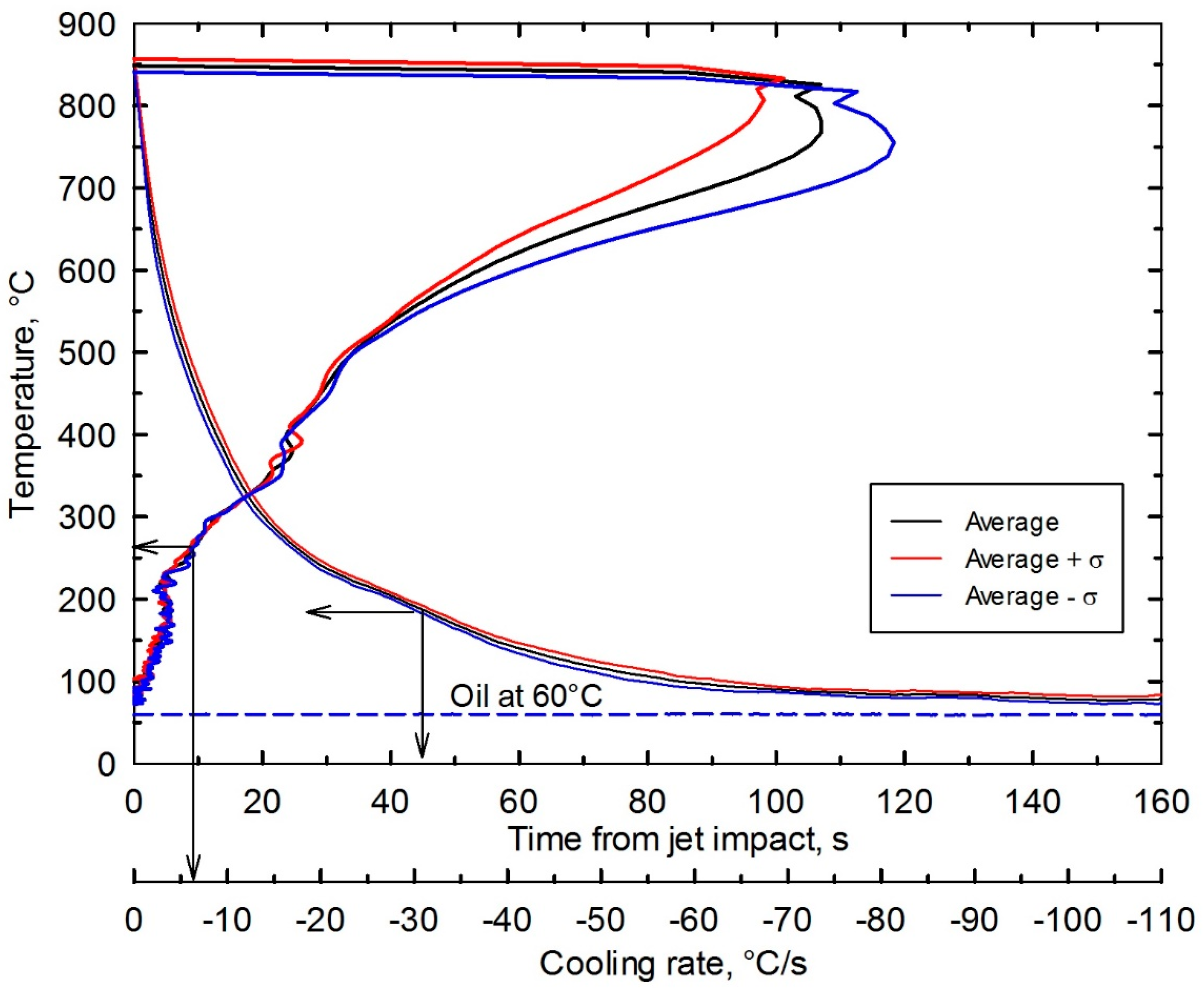
2.2.2. Diagnostic Thermal Analysis

The first step in this approach was to characterize the thermal behavior of the leaf spring during its quenching. Figure 3a schematically shows a drawing of a leaf spring that was cut into three parts: fixed, loose and center sections. They were instrumented by screwing K-type thermocouples to the surface of the leaf in the indicated points. The tip of the thermocouple was hold against the surface of the spring. An instrumented whole leaf spring had an important drawback when manually removing it from the furnace to the carousel. The thermocouple wires delayed this operation, and the leaf temperature dropped excessively before the section was immersed in the oil. In contrast, the smaller sections were heated in a portable muffle and easily moved to the carousel. Figure 3b shows a photograph during accommodation of the preheated and instrumented fixed section onto the shaper table. Figure 3c is a photograph captured during the preheating of the instrumented loose section in a muffle.

The leaf spring temperature measurements were carried out three times for every leaf section. Since there were eight thermocouples in the three sections, then we obtained 24 cooling curves.

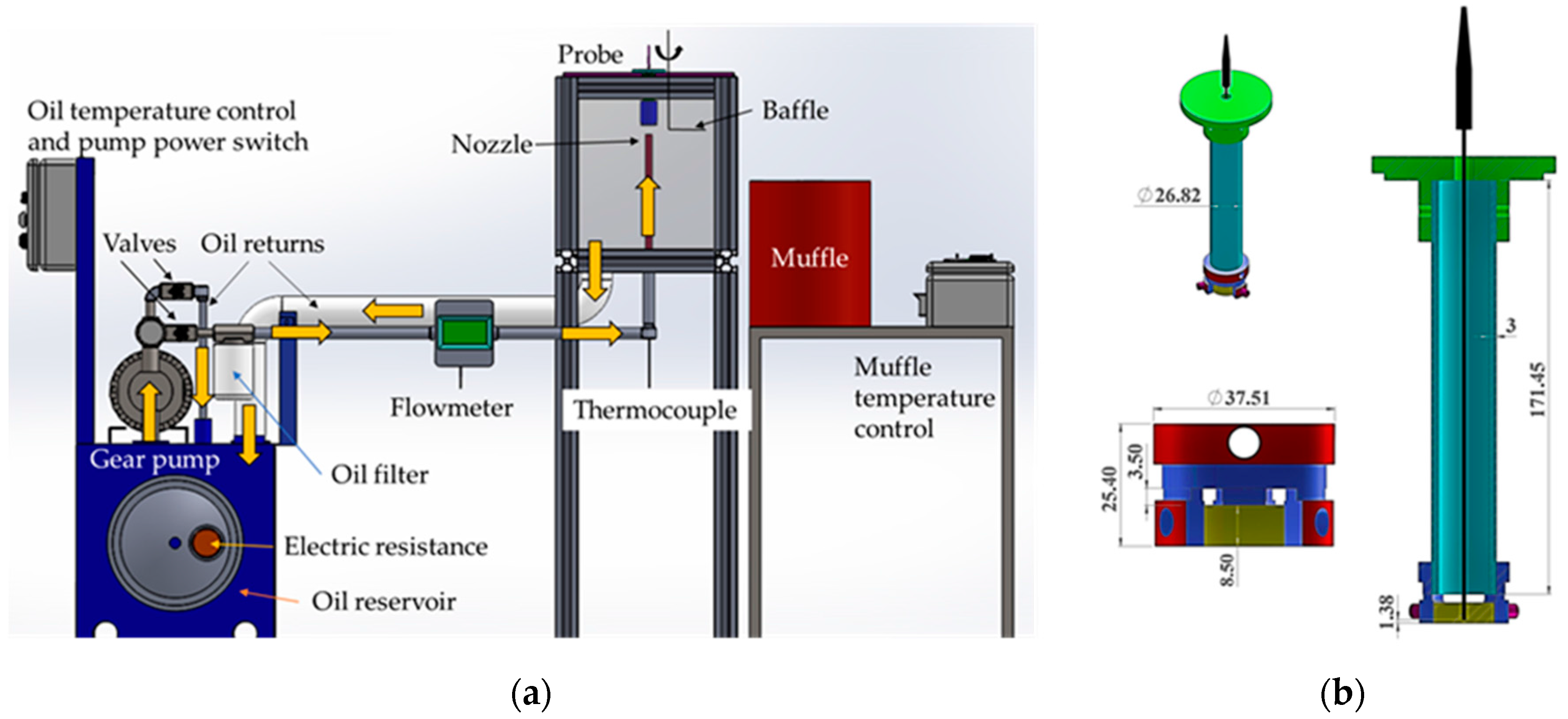
2.3. Laboratory Temperature Measurements

Laboratory thermal analyses were carried out also on DIN 51CrV4 steel samples quenched with the same oil used in plant and under controlled and recorded fluid velocities. Figure 4a shows a schematic representation of the laboratory rig to determine the rate of heat removal from steel during oil-quenching. This system was inspired in the classic Jominy End-Quench test [22] which uses a controlled water flow rate to characterize steel hardenability. This system seems to be a convenient choice to relate the already known isothermal fluid flow field of jets impinging over a flat surface with the rate of heat transfer during quenching, as it is discussed in Section 2.3. In our case, the experimental set-up includes an oil reservoir that feeds a 2 HP (1.49 kW) gear pump with an oil flowrate capacity of 40 L/min. The target oil flowrate was controlled using two valves and was measured using a turbine flowmeter (FLR6115D-BSPP, Omega Engineering Inc., Norwalk, CT, USA). An electric resistance of 4000 W and a K-type thermocouple are immersed in the oil reservoir. Both are connected to a controller unit which regulates the power consumed by the resistance to maintain the oil temperature at a set-point value. A second K-type thermocouple is connected to the line to register the oil temperature at a location near the nozzle. This nozzle is 12.7 mm internal diameter and its tip is separated from the sample surface by the same distance. The sample is a disk having a diameter of 25.4 mm and a thickness of 8.5 mm, which corresponds to the semi-thickness of the studied leaf spring.

Figure 4a also shows a moving baffle that diverted the upcoming oil while the probe was moved from the muffle to a position on top of the nozzle. Once the probe was in this position, the baffle axis was rotated and the oil impacted the pre-heated steel disk. Temperature was measured with a K-type thermocouple (TJ36-CAXL-116-G-12, Omega Engineering Inc., Norwalk, CT, USA) that was hold by compression fittings against the bottom of a hole machined from the back of the disk. The bottom of this hole was at a nominal distance of 1.8 mm from the impact surface. The thermocouple sheath diameter was 1.59 mm and the diameter of the drill was 1.7 mm. The instrumented disk was heated up in a cylindrical muffle locally built over the platform of a ceramic radiant full cylinder heater (CRFC-46/240-C-A, Omega Engineering Inc., Norwalk, CT, USA) and with the aid of a temperature controller.

The sample was hold by an artifact that is shown schematically in Figure 4b. It consists of a holder that was machined to be connected to a tube, on one side, and to hold the steel disk on the other side, using three screws that pressed the lateral surface of the disk.

The steel disk was intended to represent a semi-thickness portion of the leaf spring. Therefore, its lateral and back surface areas should be adiabatic, leaving only the front surface for heat removal. After testing several different holder designs, this artifact allowed us to approach this adiabatic condition, as it will be shown in Section 4.

The test procedure started to verify co-axial alignment between nozzle and holder. An aluminum hollow cylinder was machined ad-hoc to fit the diameters of nozzle and holder. Therefore, this cylinder allowed us to adjust co-axial alignment as well as distance between nozzle and holder. Thereafter, the instrumented steel disk was heated up to austenitization temperature. At the same time, the oil was also being heated up at a desired set-point. Before the probe reached the target temperature, the pump was on to establish a given oil flowrate. The baffle was located above of the nozzle, diverting the oil flow. The disk reached the wished temperature and was hold at this temperature for 3 min. The probe was taken out from the muffle to place it above the nozzle and the baffle axis was rotated. Oil impacted the preheated disk and the thermal history was recorded. The Plexiglas box that contained the nozzle was closed from the top to prevent oil flaming during the test. The experimental conditions include the study of the effect of initial steel temperature, oil velocity and oil temperature on the heat flow curve, and are shown in

Table 5. Laboratory conditions for oil-quenching experiments.

Initial Temperature TI (°C)	Impact Velocity VI (m/s)	Oil Temperature Tf (°C)
800	0.9	60
850
880
900
850	0.4	60
	0.9
	1.3
	2.0
850	0.9	50
		60

. Initial temperature of steel is just at the start of oil-quenching, i.e., after the air-cooling period. The impact velocity of oil jet on the surface of the disk, V_I, was corrected for the gravity acceleration, g, because the flow is upward. The expression was obtained from Bernoulli’s equation and is given by,

$$V_{\mathrm{I}}={\left(V_{\mathrm{N}}^2 -2gh\right)}^{1/2},$$

(2)

where V_N is the oil velocity at the exit of the nozzle (=Q/A_N) which depends on the oil flowrate, Q, and the cross section area of the nozzle, A_N; and h is the distance between the nozzle exit and the impact surface.

2.4. Connection between Fluid Flow and Heat Transfer

Relationships between the rate of fluid flow and the associated rate of heat transfer between a solid surface and a fluid are not new. Reynolds-Colburn analogy between shear stress and heat transfer is very useful in obtaining a first approximation for heat transfer in cases in which the shear stress is “known”. This analogy is not a physical law but it is a convenient analytical tool based on the hypothesis of the mechanism of heat transfer and shear stress [23]. It states the following relationship between convection and transferred to wall quantities:

$$\frac{\mathrm{heat}\mathrm{flux}\mathrm{to}\mathrm{wall}}{\mathrm{convection}\mathrm{heat}\mathrm{flux}}=\frac{\mathrm{momentum}\mathrm{flux}\mathrm{to}\mathrm{wall}}{\mathrm{convection}\mathrm{momentum}\mathrm{flux}},$$

(3)

which can be represented by the equation,

$$\frac{q_{\mathrm{w}}}{\rho v_{\mathrm{f}}{C}_{\mathrm{p}}\left(T_{\mathrm{f}}-T_{\mathrm{w}}\right)}=\frac{{\tau }_{\mathrm{w}}}{\rho v_{\mathrm{f}}^2},$$

(4)

where ρ, v_f, C_p and T_f are fluid magnitudes: density, bulk velocity, heat capacity and bulk temperature, respectively; while q_w, τ_w and T_w are the heat flux, shear stress and temperature at the wall. In this analogy, the shear stress is unrelated to heat transfer, that means it can be computed from isothermal fluid flow. The use of this analogy to approach boiling heat transfer in quenching tanks has not been reported before, at least according with the best knowledge of the authors. In this paper, it is proposed an efficient analysis aimed to elucidate the fluid flow field and the rate of heat flux removed from steel pieces quenched in long standing tanks. The isothermal fluid flow calculations predicted detailed shear stress distributions on the surface of leaf springs, while the analyses of heat fluxes determined from plant and laboratory data were used to propose an empirical equation based on the Reynolds-Colburn analogy.

3. Formulation of the Model

As it was explained in Section 2.4, an analysis based on Reynolds-Colburn analogy was developed in this work. Therefore, heat transfer and oil vapor evolution during quenching were sacrificed in the numerical model for the sake of an efficient algorithm. However, boiling heat transfer was addressed using plant and laboratory measurements. The objective of this model was to obtain a detailed picture of the isothermal oil flow field in the tank, particularly near the surface of the leaf springs. The shear stress and pressure imposed by the flowing oil on the wall of the spring are results that depend on the oil velocity profile near its surface.

3.1. Governing Differential Equations

The model represents the numerical solution of the Three-Dimensional (3D) momentum and mass equations for isothermal flow under steady state conditions. Turbulence was also considered by computing time-averaged quantities through the following governing equations,

Continuity:

$$\frac{\partial \rho u_j}{\partial x_j}=0,$$

(5)

Navier-Stokes:

$$\frac{\partial }{\partial x_j}\left(\rho u_i{u}_j + p{\mathsf{\delta }}_{ij} -{\mathsf{\tau }}_{ij }-{\mathsf{\lambda }}_{ij}\right)=\rho g_j,$$

(6)

Turbulence kinetic energy, k:

$$\frac{\partial }{\partial x_j}\left[\rho k{u}_j -\left(\mathsf{\mu }+\frac{{\mathsf{\mu }}_t}{{\mathsf{\sigma }}_k}\right)\frac{\partial k}{\partial x_j}\right]=G-\rho \mathsf{\epsilon },$$

(7)

Rate of energy dissipation, ε:

$$\frac{\partial }{\partial x_j}\left[\rho \mathsf{\epsilon }{u}_j -\left(\mathsf{\mu }+\frac{{\mathsf{\mu }}_t}{{\sigma }_{\mathsf{\epsilon }}}\right)\frac{\partial \mathsf{\epsilon }}{\partial x_j}\right]=(\rho C_{1}S)\mathsf{\epsilon }-(\rho C_2)\frac{{\mathsf{\epsilon }}^2}{k + \sqrt{\mathsf{\upsilon }\mathsf{\epsilon }}},$$

(8)

where u is the time-averaged local velocity; λ_ij is the Reynolds stress tensor; x is the coordinate position; ρ, μ, and υ are the density, viscosity, and kinematic viscosity of the fluid, respectively; and G is the rate of generation of turbulence kinetic energy due to the mean velocity gradients and is defined together with other quantities in

Table 6. Variables and constants appearing in turbulence equations [24].

C1	C2	G	η	S	Sij	σk	σε
$\max \left[0.43,\frac{\mathsf{\eta }}{\mathsf{\eta }+5}\right]$	1.9	${\mathsf{\mu }}_t{S}^2$	$S\frac{k}{\mathsf{\epsilon }}$	$\sqrt{2S_{ij}{S}_{ij}}$	$\frac{1}{2}\left(\frac{\partial u_j}{\partial x_i}+\frac{\partial u_i}{\partial x_j}\right)$	1	1.2

. The oil properties are included in Table 3.

The Reynolds stress is obtained from the Boussinesq approach and considers incompressible flow. The respective equation is:

$${\lambda }_{ij} = 2{\mathsf{\mu }}_t{S}_{ij}-\frac{2}{3}\rho k{\mathsf{\delta }}_{ij},$$

(9)

where δ_ij is the Kronecker delta (=0 for i ≠ j) and (=1 for i = j). Turbulence viscosity, μ_t, was determined from the following equation:

$${\mathsf{\mu }}_t=\rho C_{\mathsf{\mu }}\frac{k^2}{\mathsf{\epsilon }},$$

(10)

This quantity was computed using the realizable k-ε model [25]. This model differs from the standard k-ε model in two important ways: (1) The realizable model contains an alternative formulation for the turbulent viscosity, and (2) a modified transport equation for the dissipation rate, ε, has been derived from an exact equation for the transport of the mean-square vorticity fluctuation. The term “realizable” means that the model satisfies specific mathematical constraints on the Reynolds stresses, consistent with the physics of turbulent flows. The realizable model considers that C_μ is not a constant but is a function of the main strain and rotation rates and the angular velocity of the system rotation and the turbulence fields, k and ε [24]. Neither the standard model nor the RNG (ReNormalization Groups) model is realizable. This model has been extensively validated for a wide range of flows [25,26], including rotating homogeneous shear flows, free flows including jets and mixing layers, channel and boundary layer flows, and separated flows. For all these cases, the performance of the model has been found to be substantially better than that of the standard k-ε model. Especially noteworthy is the fact that the realizable model resolves the round-jet anomaly; that is, it predicts the spreading rate for axisymmetric jets and that for planar jets. This is particularly useful in our case to obtain a realistic flow field in the immersed oil jets coming from multiple nozzles.

The computational domain included only the space occupied by the oil inside the feeder and tank. This domain was divided into three subdomains: (1) the feeder, (2) the tank and (3) five virtual boxes at the five carousel positions where leaves are immersed. The reason for this is to improve the computer efficiency by solving each subdomain one at a time rather than the full domain in a single run. This approach is valid because the oil flows downstream. This supports the assumption that oil velocity profile at the exit of nozzles does not depend on the velocity pattern in the tank but depends only on the flowrate at the inlet cross section area of the tube feeder. Therefore, our first step was to solve for the fluid flow in the feeder by itself, whose boundary conditions and meshing are shown in Figure 5a. In a second step, the velocity profiles computed at the exit of the respective nozzles were imposed as an inlet boundary condition when solving the governing equations for the whole tank. During this step, the shaper table, the head of downholders and the leaf springs were absent except for simple flat plates that replaced them. The justification for this was to numerically capture the overall fluid flow in the tank by carefully considering the most evident flow resistance and free flow areas. Figure 5b shows the corresponding boundary conditions and meshing. To compute the fluid flow field at the neighborhood of leaf springs, a third subdomain was formed by five virtual boxes that contained the immersed springs together with the detailed geometry of the shaper table and downholders. The size of these boxes was chosen to include conveniently the leaf springs together with the shaping tools. This choice was also validated by showing that computed results were independent from box size. The computed velocity distribution from the tank solution was considered as a boundary condition for the faces that had a net positive inflow, whereas a zero reference pressure was considered a boundary condition for those faces that had a net outflow. Figure 5c indicates the corresponding boundary conditions and meshing. Notice that numerical meshing is active only on the subdomain that is being solved for, thus avoiding discretization of the solid bodies to save computer memory and time. Regarding the non-slip wall boundary condition, the adopted strategy with the normal dimensionless distance from the wall, y+, was to consider a hydrodynamically smooth wall with roughness height, K_s = 0, and default roughness constant C_s = 0.5 that had no effect in the computation. These coefficients are defined for the Law-of-the Wall Modified for Roughness [27].

3.2. Solution Method

The governing equations were solved by the finite volume method [28] implemented in the ANSYS Fluent^TM (version 16, ANSYS Inc., Canonsburg, PA, USA, 2015), code. Every subdomain was divided into several regions to reduce skewness, improving mesh quality. The underrelaxation factor was manually changed throughout the solution process to reduce the ‘scaled’ residuals for mass, momentum and turbulence equations [28] to values that were less than 10⁻³.

4. Results and Discussion

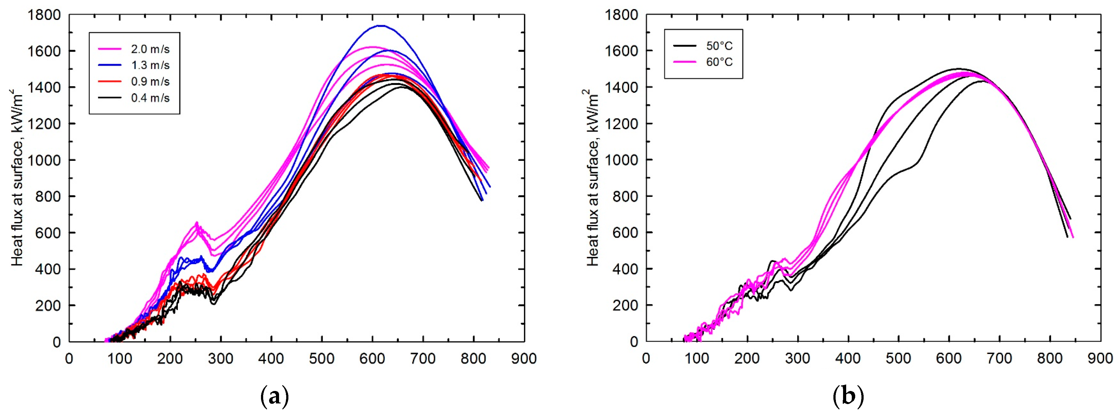
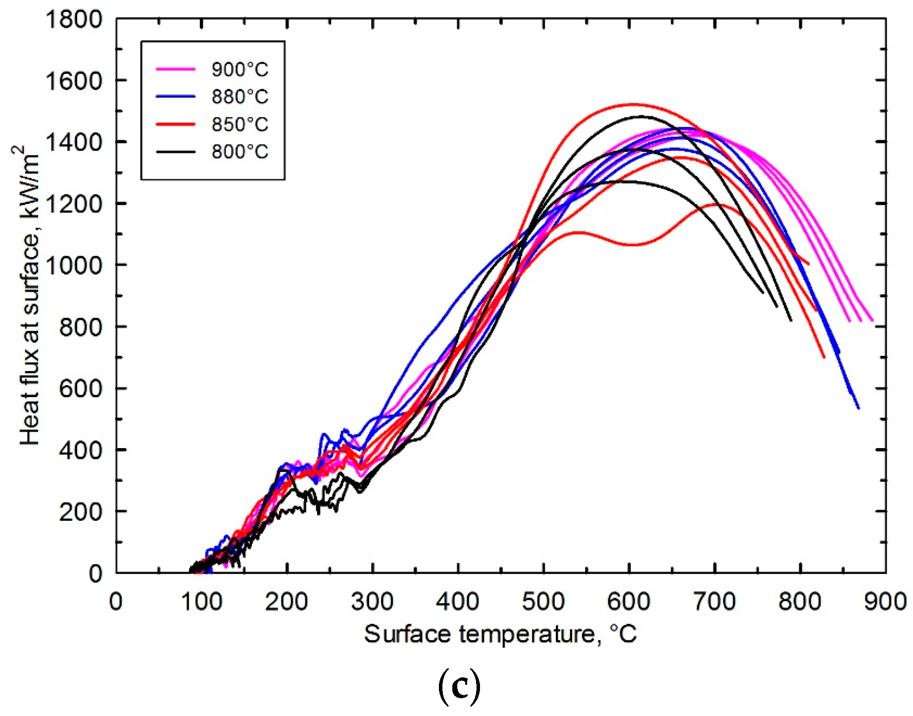
4.1. Laboratory Thermal Analysis

Laboratory thermal data for each experimental condition were obtained from at least 5 replicas. Every curve was numerically smoothed before any further processing. It was used the moving average method, choosing 5 points and averaging them according with the equation:

$$T_i^{\mathrm{av}}={{\displaystyle \sum }}_{j=i-2}^{j=i+2}{w}_j{T}_j,$$

(11)

where i and j are integers that denote time node, the weighting factors w_j are equal to 0.1, 0.2, 0.4, 0.2 and 0.1 for j = i − 2, i − 1, i, i + 1 and i + 2, respectively. After 12 smoothing sweeps, the temperature curves did not change appreciably but the cooling rate curves improved substantially, by minimizing their numerical noise. The cooling rate was estimated from the temperature smoothed data using central finite differences and no further smoothing was applied to these curves. Temperature curves for all replicas were smoothed and then they were averaged; a 95% confidence interval was computed based on standard deviation and a t-student distribution. Figure 6 shows the average temperature-time curve together with its 95% confidence interval. The limits (average ± σ) are indicated by the upper and lower curves. These results correspond to an oil impact velocity and temperature of 0.9 m/s and 60 °C, respectively, and with initial steel temperature of 850 °C. The figure shows that temperature decreases very fast until it reaches ~300 °C. This is expected since the oil boiling temperature is 290 °C. Below this temperature, boiling stops and cooling proceeds by one-phase convection. The corresponding cooling rate curves are also shown in the figure. They reach a maximum value at a high temperature. The early shoulder formed before the peak is attributed to a brief film boiling regime. Notice that uncertainty for the cooling rate is larger at temperatures above 700 °C, at which the cooling rate reaches its maximum value.

Figure 7 shows the effect of the jet impact velocity on the average temperature evolution determined from laboratory data. Similarly, to Figure 6, each curve includes its 95% confidence interval. It can be seen in Figure 7 that during the initial cooling period all curves are very close each other. However, these curves clearly separate each other at temperatures below ~350 °C where even their confidence intervals do not mutually intersect. Finally, curves become closer each other at temperatures below 100 °C as they asymptotically approach the oil temperature. The effects of the oil temperature and the initial steel temperature were not clear from the temperature-time curves. However, the boiling curves were a better choice to appreciate these effects.

The determination of the heat flux removed by the oil jet, impacting one face of the disk sample, was carried out solving the IHCP (Inverse Heat Conduction Problem) for one-dimensional transient heat conduction using Beck’s algorithm [29] implemented in the Fortran code CONTA (Sandia National Laboratories, Albuquerque, NM and Michigan State University, East Lansing, MI, USA, 1986). This analysis is valid when lateral surface of the disk is adiabatic. Furthermore, the boundary condition on the back face should be known. The adiabatic condition is the most convenient choice for our case. Therefore, the sample represented the thermal behavior of the semi-thickness of the leaf spring. Verification of each solution was carried out by solving the Direct Heat Conduction Problem (DHCP) imposing this evolving heat flux as a boundary condition and solving the heat conduction equation using the finite volume method [28] implemented in the Fortran code CONduction in DUCTs (CONDUCT) (CONDUCT, Suhas V. Patankar, University of Minnesota, Minneapolis, MN, USA, 1988). The computed temperature evolution agreed with both, measured and IHCP solution, specially above 120 °C.

Figure 8a presents the effect of oil velocity on the boiling curves determined from laboratory tests. For each oil velocity, the average temperature evolution and its 95% confidence interval were used to compute the corresponding heat flux curves. Therefore, the figure shows an average heat flux curve together with its 95% confidence interval. The figure shows that higher heat fluxes result from higher impact velocities, as expected. The curves present some noise at temperatures below 300 °C. The reason for this is not clear, but it may be due to the evolution of latent heat during solid phase transformation that could rise the steel temperature during quenching. Figure 8b shows the effect of oil temperature on the heat flux. A significate difference between heat fluxes was found in the temperature range of 300 °C to 450 °C. The heat flux for oil at 60 °C is above the one obtained using oil at 50 °C. Presumably because oil viscosity decreases with temperature. A lower oil viscosity allows an easier growth and detachment of oil vapor bubbles from the steel surface, increasing the rate of supply of cold liquid to the hot surface [30]. Figure 8c shows the effect of initial steel temperature just before jet impact. It is seen that these curves have the same shape but they are shifted to the left side for lower initial temperatures. The wide confidence interval at the heat flux maxima makes it difficult to claim an effect of initial temperature over maximum heat flux; however, in the temperature range of 200 °C to 300 °C, a lower heat flux is associated to samples with a lower initial temperature, as expected.

Regarding validity of the adiabatic boundary condition at non-active faces of the steel disk, Figure 4b shows that sample is touched by three screws only. These screws cool down simultaneously with the sample and therefore the rate of heat input is minimum. Lateral and back faces cool down by air natural convection and radiation but the rate of heat transfer to air is less than 10 kW/m² at a surface temperature of 500 °C and decreases with this temperature. It is seen in all plots of Figure 8 that heat fluxes are ~100 kW/m² at a surface temperature of 150 °C. Therefore, the heat flux that may cross through non-active surfaces is negligible.

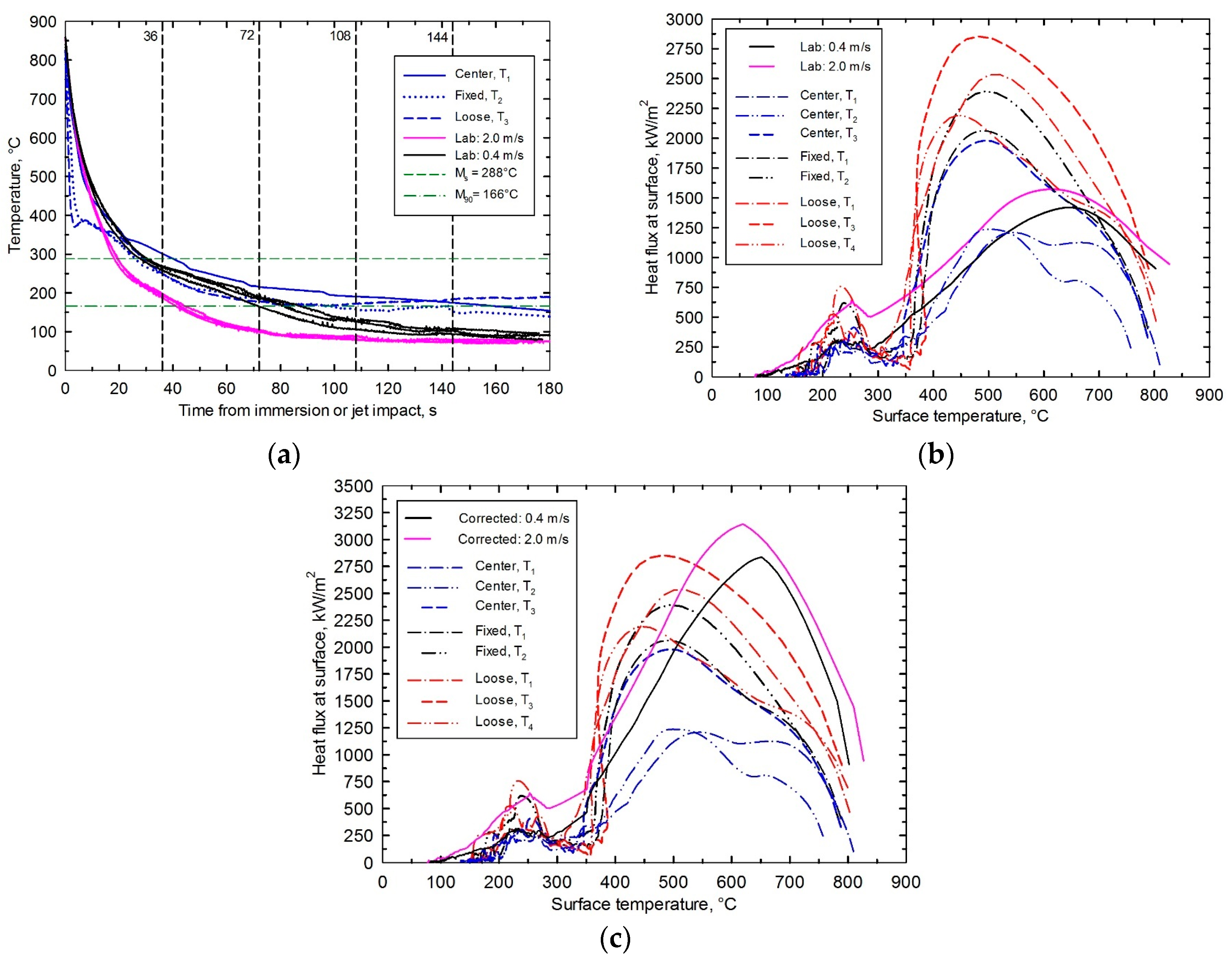
4.2. Plant versus Laboratory Thermal Analyses

The temperature error for plant measurements was larger than for the corresponding laboratory data. However, fixed and loose sections generally showed larger cooling rates than those measured for the center section. Figure 9a shows a comparison of the temperature evolution measured in plant versus the one measured in laboratory. Plant temperatures are representative of measurements for each leaf section, center, fixed and loose. The figure also shows the times at which the leaf springs reach every position in the carousel: 0 s, 36 s, 72 s, 108 s, and 144 s, leaving out the tank after 180 s. Laboratory measurements include the results for the lowest and highest oil impact velocities. It is useful to recall that leaf thickness is 17 mm while laboratory sample thickness is 8.5 mm. As it was mentioned before, this sample represents the leaf semi-thickness since only one face is active for oil cooling. Further, it should be recalled the position of thermocouples: in plant, they were screwed against the leaf surface, while in laboratory they were inserted through a hole in the back of the disk to a depth of 1.8 mm from the oil cooled surface. In the figure, plant temperatures decrease very fast in comparison with laboratory measurements, except for the center section of the leaf. The slopes of plant temperature curves change abruptly just below 400 °C, while the slopes of laboratory temperature curves change more smoothly until reaching 300 °C. Figure 9a indicates the temperatures for start and end of martensitic transformation, M_s and M₉₀, respectively. In the figure, it is seen that plant temperatures barely reach the end of martensite formation after 180 s. In contrast, laboratory temperatures decrease well below their plant counterparts after only 100 s. This is attributed to the oil velocity: In laboratory tests, the oil impact velocity is constant during the whole test; but in plant tests the oil velocity changes depending upon the leaf position in the tank, as it will be shown in the next section. To properly compare the previous results, the corresponding boiling curves were determined using the solution of the IHCP as before. Figure 9b shows the heat flux as a function of the computed surface temperature for all plant measurements and for the lowest and highest oil velocity laboratory cases. The major difference between these results is at high temperatures. The magnitude and dispersion of plant heat fluxes are much larger than the corresponding values for laboratory tests. The center section had maximum heat fluxes as low as 1200 kW/m² while loose section heat fluxes almost reach 2800 kW/m². These results contrast with maximum heat fluxes between 1400 kW/m² and 1550 kW/m² obtained in laboratory tests. On the other hand, at surface temperatures below 300 °C the laboratory heat fluxes surpass the corresponding plant values. There is only some heat flux perturbation that was found in thermocouples T₄ loose section and T₂ fixed section. Analyzing the oil velocity in both systems, laboratory test should have had larger heat fluxes, at least for the impact velocity of 2.0 m/s. In plant, the oil mean velocity at the exit of the nozzles is only 1.67 m/s as it can be estimated from data from Table 4 and recalling that input oil velocity is 0.5 m/s. Once the oil enters the tank its velocity decreases very fast with distance, as it will be shown in the next section. The authors attribute these larger heat flux values to the Taylor wavelength. This concept explains the difference of heat fluxes based on the surface area size of the samples. During the transitional boiling regime (at temperatures above those for maximum heat flux) the hot solid surface is almost blanketed with vapor. The vapor tries to buoy up, and it does in big slugs forming unstable columns or vapor jets that form and collapse intermittently under the liquid pressure. The Taylor instability is the collapse process of these emerging jets and the corresponding Taylor wavelength is the distance between jets that for a one-dimensional wave is given by the following equation [31]:

$$\mathsf{\lambda }=2\mathsf{\pi }\sqrt{3}{\left[\frac{\mathsf{\gamma }}{g\left({\rho }_{\mathrm{f}}{-\rho }_{\mathrm{g}}\right)}\right]}^{\frac{1}{2}},$$

(12)

where γ is the surface tension of oil, reported by the supplier as 0.033 N/m, and densities of fluid and gas are, ρ_f = 827 kg/m³ and ρ_g = 4.3 kg/m³. The Taylor wavelength was calculated as 2.2 cm. This means that the laboratory sample, 2.54 cm diameter, was only 1.2 times larger than λ. We can imagine that there will only be one single vapor jet detaching from the surface. In contrast, the leaf spring was 7.5 cm wide, considering its shortest dimension. This accommodates for more than 3 times the value of λ. Therefore, several vapor jets would be forming in the plant sample, improving heat transfer.

Our laboratory results can be corrected for this effect. Lienhard IV and Lienhard V [31] presented a plot in their book, which shows that the maximum pool boiling heat flux, for a given system, is independent from the surface area size of heater if this size is at least three times λ. Below this limit, experimental data indicate a decrease in the maximum heat flux.

For our laboratory sample, we read in that plot a heat flux that is half the value the expected one for an “infinite” surface. Considering that this full correction is applicable for the maximum heat flux, and that the Taylor instability does not exist during one-phase cooling, we propose the following empirical corrections for laboratory boiling curve.

For temperatures T_a ≤ T ≤ T_max,

$$q^{\mathrm{corr}}{=q}^{\mathrm{orig}}\left\{1+{\left[\frac{{T-T}_{\mathrm{a}}}{T_{\max } {-T}_{\mathrm{a}}}\right]}^{ma}\right\},$$

(13)

and for temperatures T_b ≥ T > T_max,

$$q^{\mathrm{corr}}{=q}^{\mathrm{orig}}\left\{1+{\left[\frac{T_{\mathrm{b}}-T}{T_{\mathrm{b}} {-T}_{\max }}\right]}^{mb}\right\},$$

(14)

where T_max is the temperature at the peak heat flux, q_orig and q_corr are the original and corrected heat fluxes, respectively; T_a and T_b are the lowest and highest temperatures where correction applies. In our case, they were taken as 350 °C and the initial sample temperature, respectively. The exponents ma and mb were both fit equal to 1/3. The proposed empirical equations multiply only the peak heat flux by a factor of 2 and modify the rest of the curve by a smaller factor that decreases in proportion to the temperature difference, |T − T_max|, reminding a level rule. Figure 9c shows the data of Figure 9b but with corrected laboratory heat fluxes. The magnitude of heat flux is now above the corresponding plant values, as it is expected from the low oil velocities in most of the tank. The maxima heat fluxes in plant are shifted towards lower temperatures. This is a result of the observed large initial slopes in the temperature-time curves and their abrupt change just below 400 °C, see Figure 9a. Further research is required to elucidate this behavior.

4.3. Fluid Flow Analysis

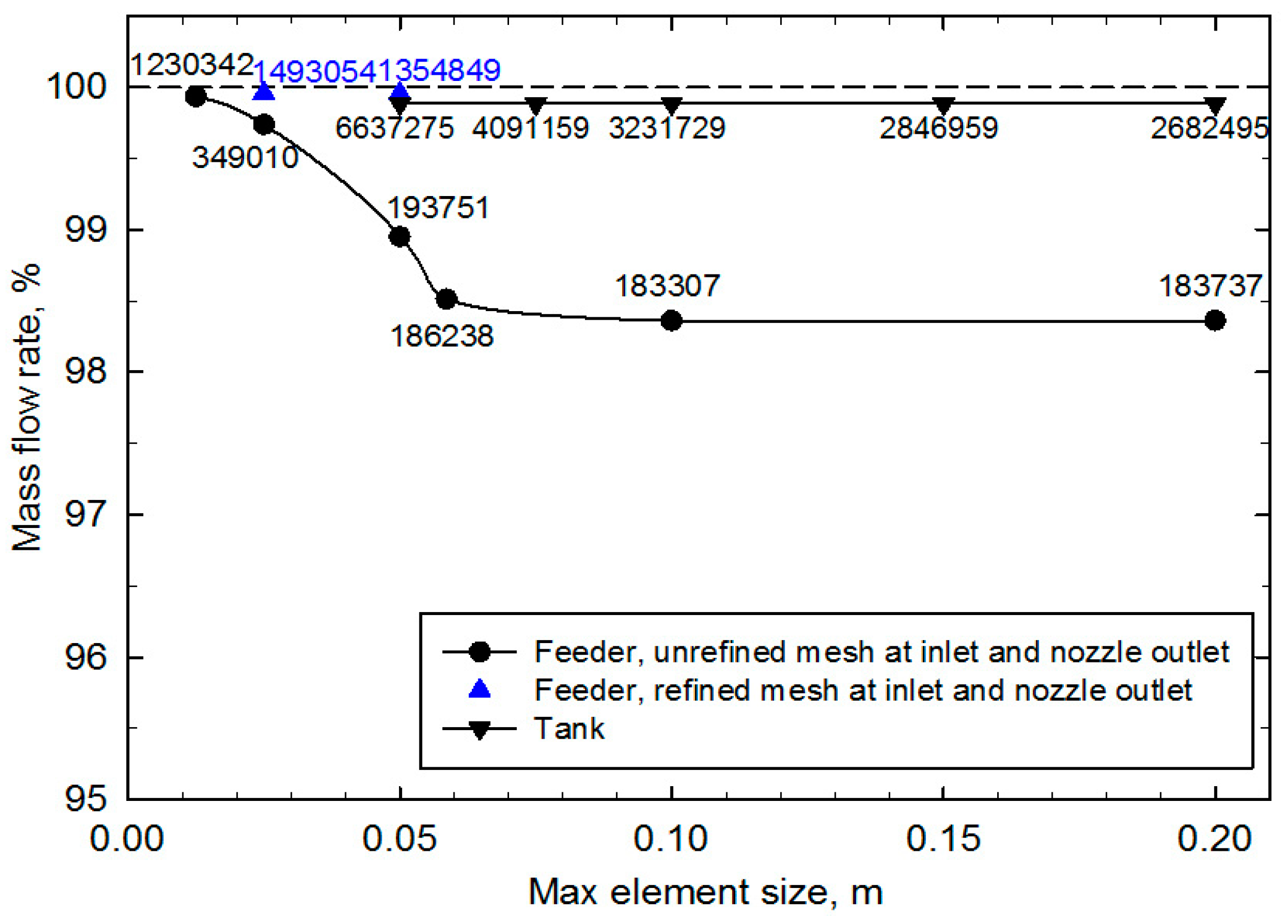
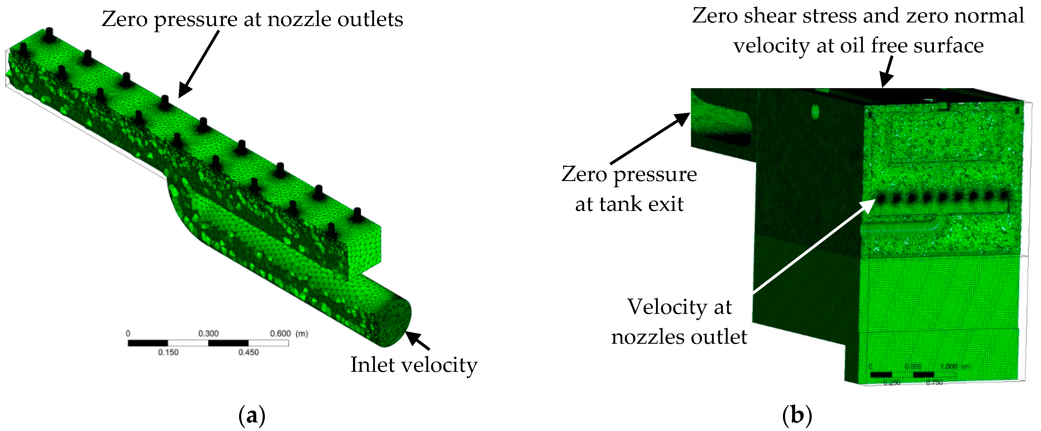
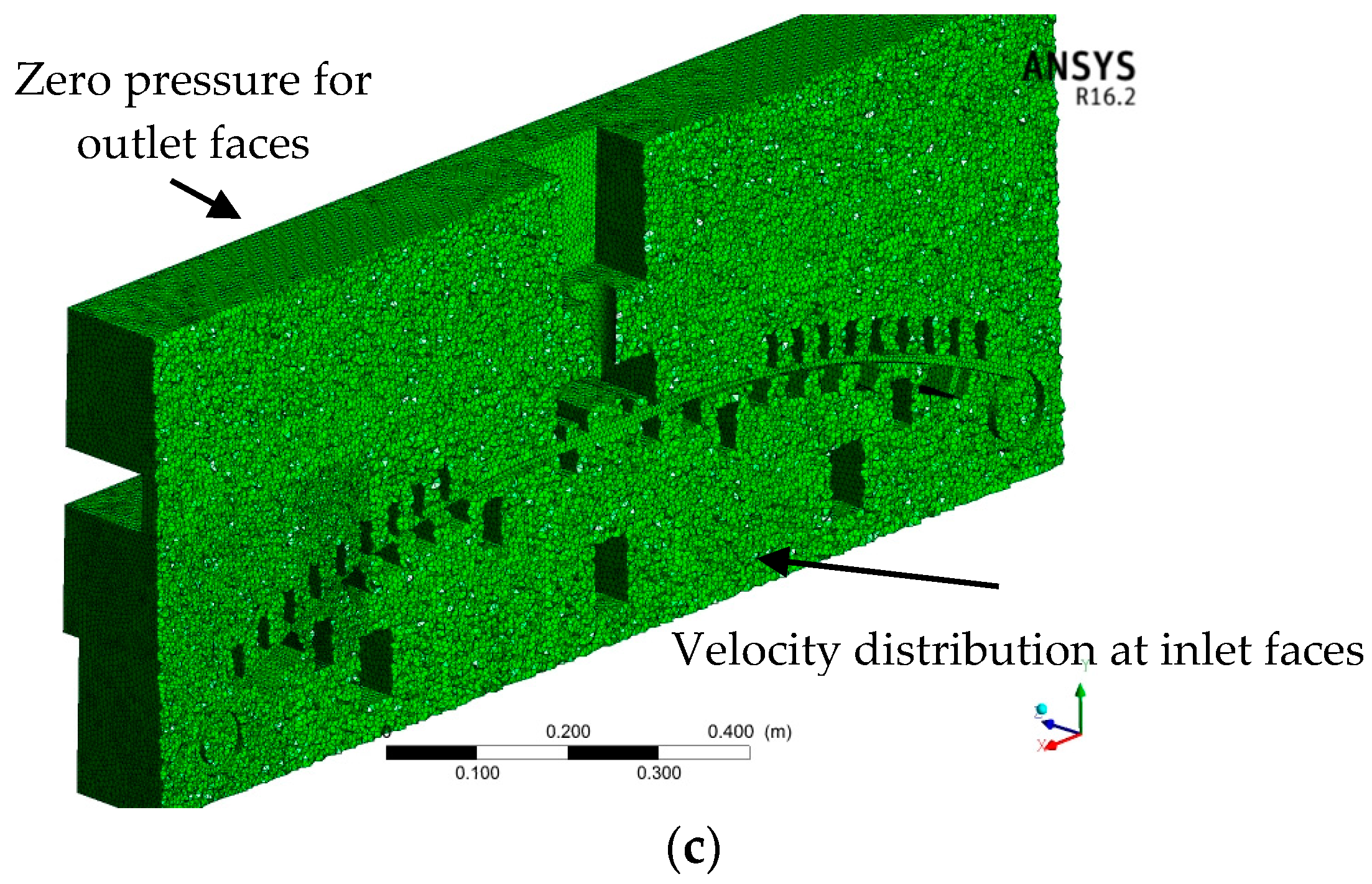
This section presents the results of fluid flow in the original system using both methods, the proposed “cascade” calculations versus the full domain calculations. Numerical simulations were then carried out using only the “cascade” calculations for the proposed cases shown in

Table 7. Characteristics of the analyzed quenching systems.

Case	Characteristics
Original	Feeder with two rows of nozzles pointing upward. Oil average velocity at feeder tube, 0.5 m/s.
Higher flowrate	Original feeder. Oil average velocity at feeder tube, 1 and 5 m/s.
Baffles installed around carousel	Original feeder and oil velocity at feeder tube, 0.5 m/s.
Shallow tank	Original feeder and oil velocity at feeder tube, 0.5 m/s. Depth of tank in carousel area, 1.73 m.
Nozzle rows at 90°	Feeder with nozzle rows at 90° from each other. Oil average velocity at feeder tube, 0.5 m/s.

. This table includes, in addition to the original system operating at its current oil flowrate, the system operating at twice and at ten times this flowrate. Another modification consisted of placing baffles along the periphery of the carousel. It was thought that they would divert the oil to flow parallel to the carousel faces rather than crossing them. A further modification was to shorten the tank depth. The idea behind this change was to reduce the cross-sectional area for fluid flow, which would lead to an increase in oil velocity in the tank.

Finally, a separate case considered a modification in the location of nozzles. The original feeder has two parallel rows of nozzles pointing upward, but the modified one has two rows of nozzles at 90°, one pointing upward and the other pointing horizontally.

4.3.1. Mesh Quality

The sensitivity of the total mass flowrate with the maximum cell size and number of elements for the feeder and tank in the original case is represented in Figure 10. Mesh refining at the feeder inlet and nozzle outlets improved the accuracy to compute the mass flowrate. The feeder was discretized with a total of 1,354,849 elements to obtain mesh-independent results. Mesh quality is given by an average skewness of 0.228 with a standard deviation of 0.119. Figure 10 shows that the tank results were all mesh-independent. This subdomain was divided into a total of 6,637,275 elements, which have an average skewness of 0.211 and standard deviation of 0.128. Finally, the third sub-domain includes the 5 virtual boxes. Each one was discretized with 3,434,308 elements having an average skewness of 0.230 and standard deviation of 0.123.

In contrast, the full system was discretized into ~48.6 million elements to obtain a similar element size distribution and average skewness compared with all the subdomains used for the proposed “cascade” computing sequence.

Table 8. Number of elements and computing time for fluid flow simulation in a quench tank using “cascade” calculations versus full system calculations. Computer runs were carried out on an 8-core microprocessor Intel Xeon ESG45, 2.4 GHz and 32 GB of RAM.

Subdomain	Millions of Elements	Running Time—“Cascade” (h)	Millions of Elements	Running Time—Full System (h)
Feeder	1.4	1.1	48.6	168
Tank	6.6	12.2
Box 1	3.4	1.9
Box 2	3.4	1.4
Box 3	3.4	1.6
Box 4	3.4	1.7
Box 5	3.4	1.8

shows a comparison of the number of elements and the total computing time between these methods. The “cascade” calculations require a maximum of 6.6 million elements per run, whereas the full system needs a total of 48.6 million elements. This makes a tremendous difference in terms of computer memory, file management and storage requirements. The total running time takes 21.7 h in “cascade” method, whereas this run lasts 168 h in the full system calculations to obtain similar convergence and results.

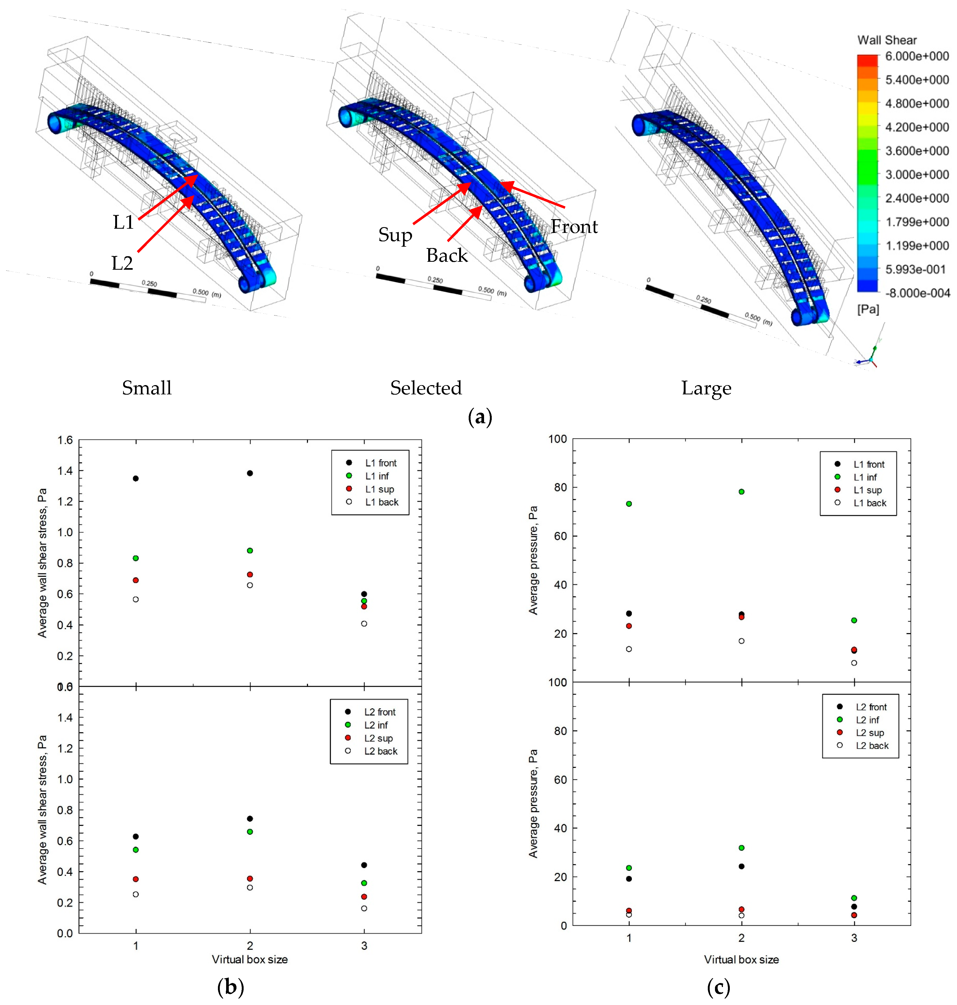
4.3.2. Choice of Virtual Box Size

The virtual box size was selected to include both leaf springs, with dimensions to match or exceed the shaping tools surface boundaries. Three box sizes were considered to carry out a sensitivity analysis, small (1458 × 434 × 221), selected (1458 × 570 × 221) and large (1818 × 570 × 286), all in mm. Figure 11a shows the computed maps of shear stress on the surface of both leaf springs obtained using three different virtual box sizes. It can be noticed that the small and selected boxes led to mutually similar results, while the large box results did not fully agree with them.

Figure 11b,c are plots of the average wall shear stress and pressure, respectively. The averages were taken over each of four leaf faces. These plots confirm the agreement between the results obtained with small and selected boxes. The faces of the selected box size are close enough to the leaf surface to properly transmit the oil velocity information to this surface, and are also far enough from the leaf body to include a better representation of the tools that hold it.

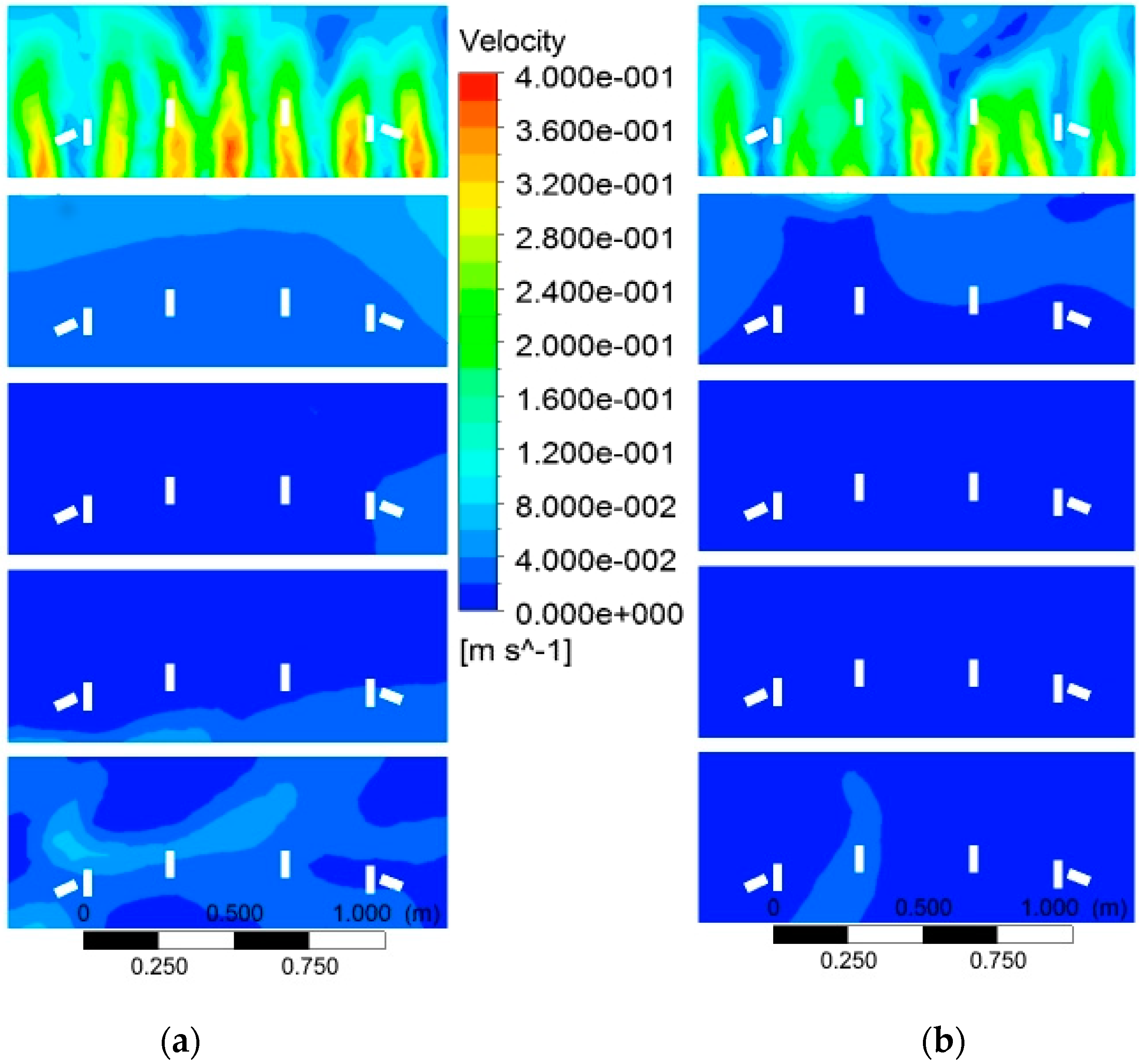
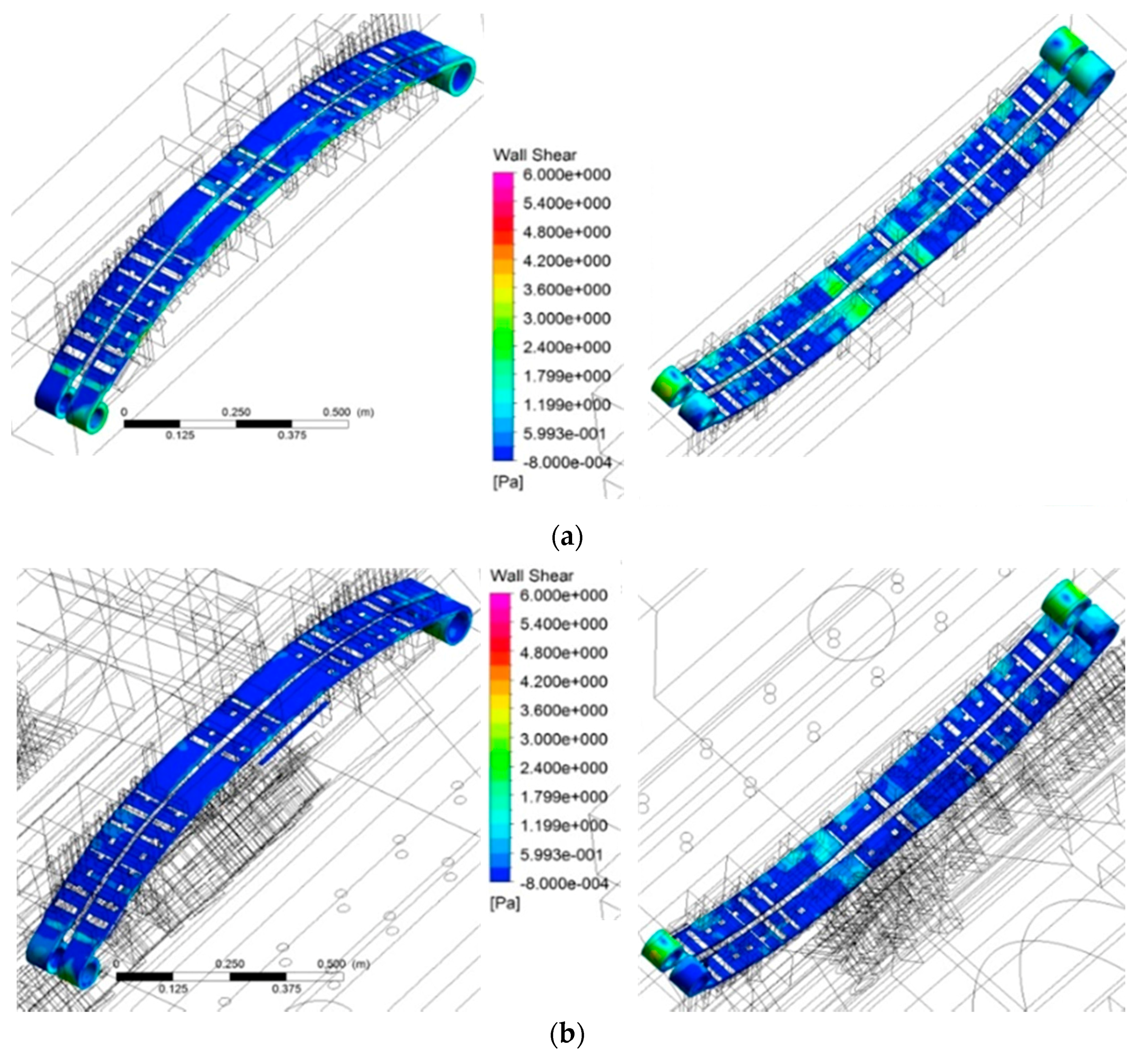
4.3.3. Fluid Flow Maps for Original Case

Figure 12a–d show a comparison between the results obtained with the “cascade” and full system methods. Figure 12a represents the shear stress distribution computed using the “cascade” method at the surface of the leaf springs at carousel position number 1, and Figure 12b shows the corresponding results but using the full domain calculations. In both cases, the wall shear is larger at the spring eyes because the oil flows freely there. In addition, a shadow effect in the wall shear distribution is present. This is a result of directional flow passing through the leaf springs. Figure 12c,d show the wall shear stress element frequency obtained with the full domain and “cascade” methods for first and second carousel positions. In these plots, the frequency represents the number of volume elements which wall shear is within one class number. Each class number is equivalent to 0.01 Pa. These figures show that there is a fair agreement between “cascade” and full solutions. The “cascade” solution was sensitive enough to recreate the response of the shear stress distribution to both, leaf and carousel positions. The analysis presented in this paper was obtained using the “cascade” method.

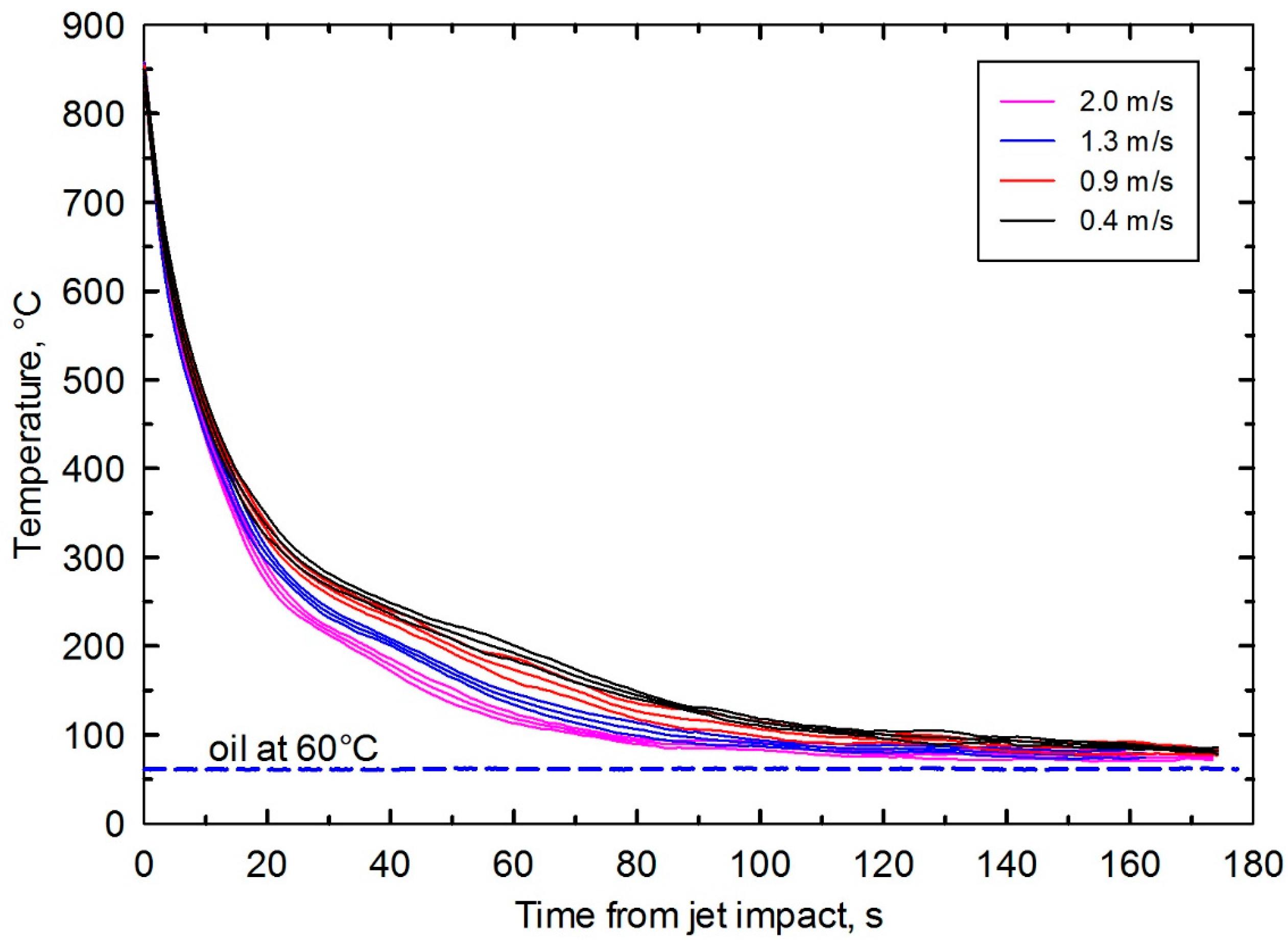
4.3.4. Effect of Oil Flowrate

Figure 13a–c show the computed velocity norm maps at the frontal face of the 5 virtual boxes, according with Figure 2a starting from position 1 at the top, when feeding oil at three different velocities 0.5 m/s, 1 m/s and 5 m/s, respectively. The frontal face of a box is the one that sees radially out, and it receives the oil that comes from the feeder. The projecting shaper table is shown by the white rectangular spots. Figure 13a corresponds to the original case and shows that the first box is essentially the only one that receives the oil at a relatively higher velocity, ~0.04 m/s. Boxes 2 to 5 receive oil at very low velocities. This is consistent with the measured plant temperature evolution presented in Figure 9a. In these results, the measured rate of cooling in the first carousel position was the highest. Figure 13b shows the velocity maps when the oil is fed at 1 m/s. Once again, the first box receives the oil at the highest velocity, leaving the other boxes with the lowest flow velocity. Figure 13c is an extreme case in which oil is input at 5 m/s. The oil velocity at the first box increases at values of approximately 0.40 m/s. Velocity is also increased in all other boxes. This solution might work for improving productivity. However, the high and non-uniform oil velocity at the first box may lead to localized high cooling rates with undesirable quality results.

4.3.5. Effect of Baffles at Carousel Periphery

Figure 14a,b show the computed velocity norm maps on the frontal faces of the virtual boxes for the original case and for the modified carousel with baffles. The original feeder was used in both cases. The figures show that there is no significant difference between these cases. This is attributed to the depth of the tank. Although the baffles were placed to block the oil flow through the interior of the carousel, the still relatively large cross-sectional area of the tank led to low oil velocity, as in the original case.

4.3.6. Effect of Tank Depth

A decrease in the tank depth was aimed to reduce the tank cross-sectional area for the oil to flow, increasing its velocity. Figure 15a,b show the computed norm velocity maps for the original case and for the tank with a shortened depth. A comparison between the velocities shows that they are essentially equivalent systems. This means that the sole reduction of the tank depth is insufficient to modify the oil velocity pattern in the virtual box faces. The oil flows mostly through the interior of the carousel.

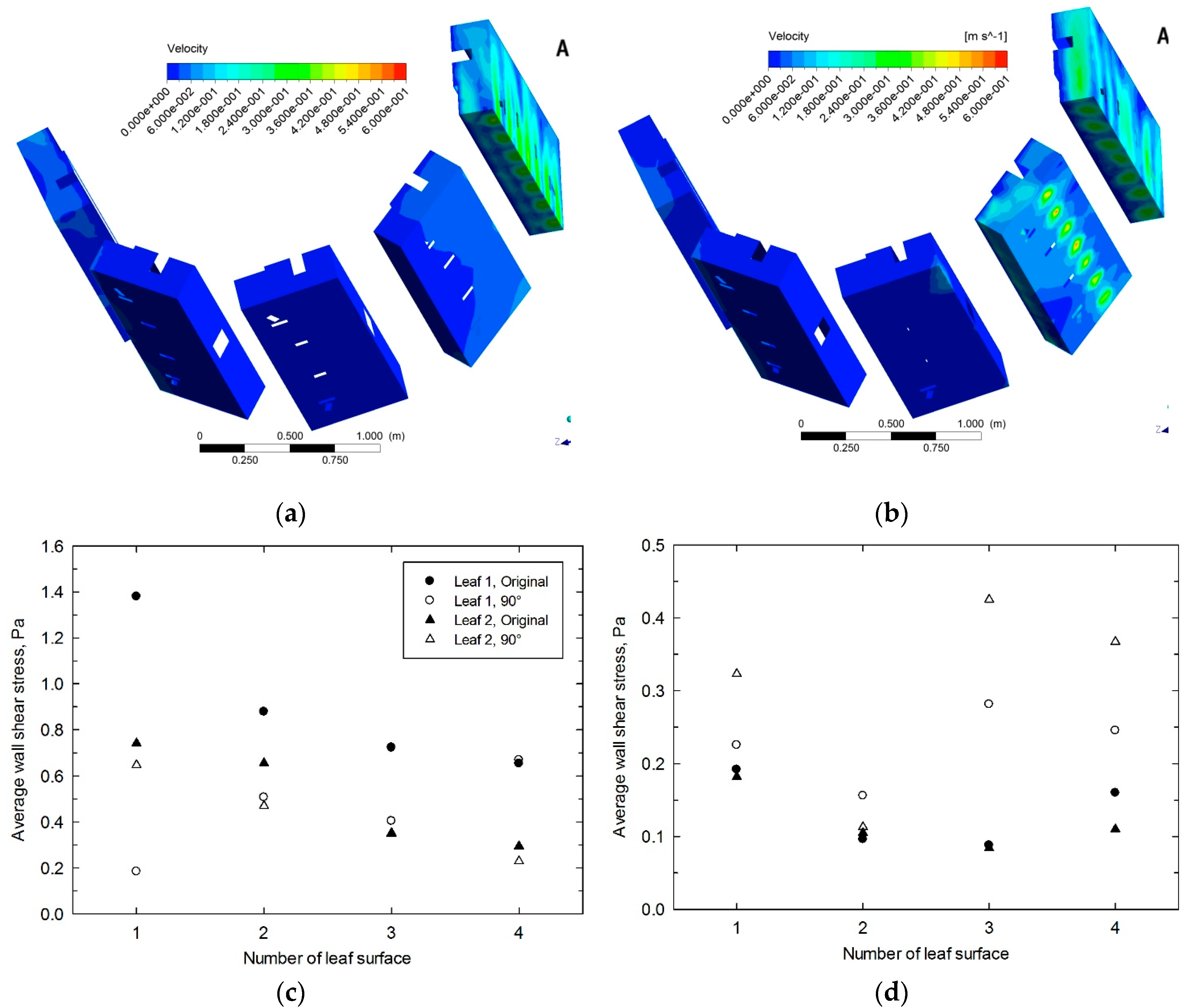
4.3.7. Effect of Nozzle Direction

Figure 16a,b show computer digital representations of the original feeder and the modified one, respectively. In both figures, the computed velocity vector distribution is seen at the nozzle outlets. Figure 16c,d show the computed velocity norm maps at the frontal face of the virtual boxes when using a feeder as in Figure 16a,b, respectively. Notice that in Figure 16d, the second box receives oil at a relatively higher velocity compared with the second box in Figure 16c. This is the result of relocating the second row of nozzles. In contrast, the first box receives oil at a lower velocity compared with the first box in Figure 16c. This solution may be suitable for our purpose because it improves the oil velocity in the second box, in which the measured cooling rate decreased, as shown in Figure 9a. Figure 17a,b show the computed velocity maps for the cases in Figure 16c,d, respectively, but in a 3D view, to show velocity maps in additional faces. Again, it is seen that oil velocity in box 1 is larger for the original system but in box 2 the situation is opposite. Figure 17c,d show the computed average wall shear on each of the 4 faces of both leaf springs when they are in box 1, Figure 17c, and in box 2, Figure 17d. It is clear from these plots that wall shear stress is larger for the original case in box 1 but the 90° nozzle rows case dominates in box 2. The inferior (face 2) and superior (face 3) leaf surfaces represent the main heat removal areas. The change in nozzle configuration represents, for box 1, a decrease in shear stress in these areas from 0.4–0.9 Pa to 0.4–0.5 Pa. However, it represents for box 2 an increase in shear stress from 0.08–0.11 Pa to 0.10–0.43 Pa. To find out if this increase is high enough to compensate the decrease in the shear stress in box 1, it is necessary to have a relationship between heat flux and wall shear stress.

Before stepping forward to heat transfer analysis, it is interesting to notice that Figure 14, Figure 15, Figure 16 and Figure 17 show that oil velocity drops sharply after box 1. This means that most of the momentum and turbulence kinetic energy of the feeding jets are dissipated in a relatively short distance from the nozzles outlet. Only box 1 receives oil at a moderate velocity. These results offer an explanation on the resulting high cooling rates that were measured in leaf sections during the first seconds, see Figure 9a. In contrast, the measured cooling rates corresponding to positions of boxes 2 to 5 were very small. This is consistent with a predicted very low oil velocity flowing through these boxes.

4.4. Isothermal Fluid Flow and Heat Flux

The Reynolds-Colburn analogy, Equation (4), is our starting point to obtain a relationship between the heat flux and the wall shear stress, and it can be rewritten as:

$$\frac{q_{\mathrm{w}}}{C_{\mathrm{p}}\left(T_{\mathrm{f}} {-T}_{\mathrm{w}}\right)}=\frac{{\mathsf{\tau }}_{\mathrm{w}}}{v_{\mathrm{f}}},$$

(15)

This equation is the basis to postulate the following empirical equation:

$$q_{\mathrm{w}}{=q}_{\mathrm{w}}^1{\mathsf{\tau }}_{\mathrm{w}}^n,$$

(16)

In this power law equation, $q_{\mathrm{w}}^1$ is numerically equal to the heat flux when the wall shear stress is equal to 1, and n is a real number; both were determined from the laboratory results that were shown in Figure 8a. In this figure, the heat flux depends on the oil impact velocity, and the corresponding curves are fairly parallel each other. These velocities led to wall shear stresses that were estimated from previous studies of jet impacting a horizontal planar surface. The early work of Bradshaw and Love [32] reports measurements of velocity magnitude and direction, static pressure, and skin friction in a circular turbulent air jet impinging normally on a flat, isothermal, surface. They found that the maximum value of skin friction shear stress occurs at a radius approximately equal to that of the jet and is about 0.006 times the jet maximum dynamic pressure. Nowadays, these results have been confirmed and accepted even for liquids impinging over flat surfaces. The authors reported that the skin friction changes from zero at the axis of the jet (r = 0) to its maximum value at the radius of the jet (r ≈ R) in a quasi-linear form. Therefore, to determine the wall shear stress for our laboratory experiments, we considered a value half the maximum shear stress, which corresponds to an arithmetic average shear stress. The gravity effect was considered in the analysis by estimating de impact jet velocity with Equation (2).

Table 9. Estimated average wall shear stress for the laboratory experiments using Bradshaw and Love results [32]. The ratio $q_{\mathrm{w}}/q_{\mathrm{w}}^1$ was obtained from Figure 8a.

Impact Velocity, VI (m/s)	Average Wall Shear Stress, τmax/2 (Pa)	${\mathit{q}}_{\mathbf{w}}{/\mathit{q}}_{\mathbf{w}}^1$	n
0.4	0.2	0.903	0.06
0.9	1.0	1	-
1.3	2.1	1.452	0.503
2.0	4.96	1.935	0.412

shows the estimated average wall shear stress for each experiment. The table also shows the estimated ratio of the heat flux divided by the corresponding heat flux at shear stress equal to one. This ratio was determined from Figure 8a by considering the heat fluxes at 250 °C. Notice that at this temperature, one phase convection is the heat transfer mechanism. However, we are applying Equation (16) to the whole boiling curve. Finally, the table shows the computed value for n using Equation (16). We present this coefficient as,

n = 0.06, for τ ≤ 0.2 Pa; and n = 0.46 (average value), for τ ≥ 1 Pa,

(17)

where n should be interpolated for a shear stress value between 0.2 Pa and 1 Pa. Furthermore, if we consider that the effect of the initial steel temperature, T_I, is to displace the heat flux curve as it was shown in Figure 8c, we use the following expression for $q_{\mathrm{w}}^1$:

$$q_{\mathrm{w}}^1=f\left(T_I-T_{\mathrm{w}}\right),$$

(18)

This equation means that $q_{\mathrm{w}}^1$ is a function of the difference between initial and wall temperatures rather than a function of only T_w. Of course, the same will be true for q_w. Equation (16) together with Equations (17) and (18) represent a relationship between the computed isothermal wall shear stress and the expected heat flux. Application of this equation to the production tank requires that the laboratory heat flux curve should also be corrected for the Taylor wavelength according with Equation (13).

Based on the computed shear stress, Equation (16) predicts that heat flux decreases in leaves of box 1 around 15% when changing the feeder from the original case to the proposed 90° rows case. However, the improvement in heat flux obtained in the leaves in box 2 is around 10%. This means that the expected overall cooling rates should be very similar for both cases. Another different design and/or operating solution should be found to improve the rate of cooling of the leaf springs.

5. Summary and Conclusions

An efficient fluid-dynamic analysis has been developed and applied to the redesign of an industrial oil-quenching tank for automotive leaf springs. The analysis is based on a proposed empirical power-law equation to relate the isothermal wall shear stress, computed numerically on the surface of the leaf springs, with the heat flux removed during their quenching. Laboratory experiments, carried out on a modified Jominy End-Quenched rig, allowed us to determine the parameters of an empirical relationship between the measured heat flux and the estimated isothermal average shear stress on the surface impacted by the oil jet. This empirical equation is based on the Reynolds-Colburn analogy and includes correction for the effect of the initial temperature of the steel. The result should be also corrected for the Taylor wavelength, that accounts for the difference in surface area size between the laboratory and plant specimens.

The numerical model predicts efficiently the isothermal velocity field in the tank, by solving the momentum and continuity equations under steady-state conditions and turbulent flow in 3D. Computer efficiency is based on “cascade” calculations in three subdomains: the oil feeder, the tank, and 5 virtual boxes that contain the leaf springs held by the appropriate tools and immersed in the tank. Therefore, the oil velocity distribution at the nozzle outlet of each subdomain was used as the inlet boundary condition for the next subdomain. Calculations were carried out in each subdomain one at a time and compared with the corresponding results when using the full domain in a single run. In both methods, meshes with similar average element size and skewness were used. In addition, the corresponding fluid flow results fairly agree. It was shown that “cascade” calculations save a considerable amount of computer memory and processing time compared with full-domain calculations, without a considerable loss of accuracy.

The computed norm velocity maps on the faces of the virtual boxes are convenient indicators to explore a potential benefit or drawback when implementing new design options. Calculating the flow field inside the boxes reveals details of the shear stress distribution on the leaf spring surfaces.

In the present work, the measured rate of cooling at several locations on the surface of a leaf spring showed that there are significate differences between these rates, particularly during the period at position 1 of the carousel. This is attributed to a non-uniform oil velocity distribution near the leaf spring. The rate of cooling decreases from positions 2 to 5. Therefore, oil velocity should be improved in these positions. The fluid-dynamic analysis of the original quenching system and most of its modifications showed little improvement of the oil velocity in the virtual boxes that contain the leaf springs. A plain increment in the oil flowrate increases the fluid velocity only in virtual box 1 but remains with little change in the other boxes. A reduction of the cross-sectional area of the flow path by either introducing baffles to block the flow through the center of the carousel or reducing the tank depth was insufficient to improve the liquid velocity at the other boxes. The better case was the feeder with nozzle rows 90° from each other. In this case, the oil velocity in the second carousel position increased with respect to its value in the original case. However, a detailed heat transfer analysis using the proposed empirical equation showed that no major benefit could be obtained from this solution. More possible solutions can be conveniently simulated and evaluated using the proposed “cascade” calculations.

References

1. Canale, L.D.C.F.; Totten, G.E. Quenching technology: A selected overview of the current state-of-the-art. Mater. Res. 2005, 8, 461–467. [Google Scholar] [CrossRef]
2. Totten, G.E. Quench Process Sensors. In ASM Handbook; Dossett, J., Totten, G.E., Eds.; ASM International: Materials Park, OH, USA, 2013; pp. 192–197. [Google Scholar]
3. Gür, C.H.; Şimşir, C. Simulation of quenching: A review. Mater. Perform. Charact. 2012, 1, 1–37. [Google Scholar] [CrossRef]
4. Totten, G.E.; Bates, C.E.; Clinton, N.A. Handbook of Quenchants and Quenching Technology; ASM International: Materials Park, OH, USA, 1993; pp. 339–411. [Google Scholar]
5. Garwood, D.R.; Lucas, J.D.; Wallis, R.A.; Ward, J. Modeling of the flow distribution in an oil quench tank. J. Mater. Eng. Perform. 1992, 1, 781–787. [Google Scholar] [CrossRef]
6. Halva, J.; Volný, J. Modeling the flow in a quench bath. Hut. Listy 1993, 48, 30–34. [Google Scholar]
7. Bogh, N. Quench Tank Agitation Design Using Flow Modeling. In Proceedings of the International Heat Treating Conference: Equipment and Processes, Schaumburg, IL, USA, 18–20 April 1994; Totten, G.E., Wallis, R.A., Eds.; ASM International: Materials Park, OH, USA, 1994; pp. 51–54. [Google Scholar]
8. Kernazhitskiy, S.L. Numerical Modeling of a Flow in a Quench Tank. Master’s Thesis, Portland State University, Portland, OR, USA, 2003. [Google Scholar]
9. Kumar, A.; Metwally, H.; Paingankar, S.; MacKenzie, D.S. Evaluation of Flow Uniformity around Automotive Pinion Gears during Quenching. In Proceedings of the 5th International Conference on Quenching and Control Distortion at 2007 European Conference on Heat Treatment, Berlin, Germany, 25–27 April 2007; International Federation for Heat Treatment and Surface Engineering: Berlin, Germany, 2007; pp. 1–8. [Google Scholar]
10. Romão-Bineli, A.R.; Rocha-Barbosa, M.I.; Luiz-Jardini, A.; Maciel-Filho, R. Simulation to Analyze Two Models of Agitation System in Quench Process. In Proceedings of the 20th European Symposium on Computer Aided Process Engineering, Naples, Italy, 6–9 June 2010; Pierucci, S., Ferraris, G.B., Eds.; Elsevier B.V.: Naples, Italy, 2010; pp. 1–6. [Google Scholar]
11. Krause, F.; Schüttenberg, S.; Fritsching, U. Modelling and simulation of flow boiling heat transfer. Int. J. Numer. Methods Heat Fluid Flow 2010, 20, 312–331. [Google Scholar] [CrossRef]
12. Srinivasan, V.; Moon, K.-M.; Greif, D.; Wang, D.; Kim, M.-H. Numerical simulation of immersion quench cooling process using an Eulerian multi-fluid approach. Appl. Therm. Eng. 2010, 30, 499–509. [Google Scholar] [CrossRef]
13. Gao, W.-M.; Fabijanic, D.; Hilditch, T.; Kong, L.-X. Integrated fluid-thermal-structural numerical analysis for the quenching of metallic components. J. Shanghai Jiaotong Univ. Sci. 2011, 16, 137–140. [Google Scholar] [CrossRef]
14. Ricci, M.G.; Santin, G.; Cascariglia, F.; Scimiterna, E.; Parrabbi, A.; Carpinelli, A. Numerical analysis applied to thermal and fluid-dynamic quenching simulation of large high quality forgings. La Metall. Italiana 2011, 9, 3–10. [Google Scholar]
15. El Kosseifi, N. Numerical Simulation of Boiling for Industrial Quenching Processes. Ph.D. Thesis, Paris National School of Mines, Paris, France, 2012. [Google Scholar]
16. Ko, D.-H.; Ko, D.-C.; Lim, H.-J.; Kim, B.-M. Application of QFA coupled with CFD analysis to predict the hardness of T6 heat treated A16061 cylinder. J. Mech. Sci. Technol. 2013, 27, 2839–2844. [Google Scholar] [CrossRef]
17. Kopun, R.; Škerget, L.; Hriberšek, M.; Zhang, D.; Edelbauer, W. Numerical investigations of quenching cooling processes for different cast aluminum parts. J. Mech. Eng. 2014, 60, 571–580. [Google Scholar] [CrossRef]
18. Passarella, D.N.; L-Cancelos, R.; Vieitez, I.; Varas, F.; Martín, E.B. Thermo-fluid-dynamics quenching model: Effect on material properties. Blutcher Mech. Eng. 2012, 1, 3625–3644. [Google Scholar]
19. Yang, X.-W.; Zhu, J.-C.; He, D.; Lai, Z.-H.; Nong, Z.-S.; Liu, Y. Optimum design of flow distribution in quenching tank for heat treatment of A357 aluminum alloy large complicated thin-wall workpieces by CFD simulation and ANN approach. Trans. Nonferr. Met. Soc. China 2013, 23, 1442–1451. [Google Scholar] [CrossRef]
20. Banka, A.L.; Ferguson, B.L.; MacKenzie, D.S. Evaluation of flow fields and orientation effects around ring geometries during quenching. J. Mater. Eng. Perform. 2013, 22, 1816–1825. [Google Scholar] [CrossRef]
21. López-García, R.D.; García-Pastor, F.A.; Castro-Román, M.J.; Alfaro-López, E.; Acosta-González, F.A. Effect of immersion routes on the quenching distortion of a long steel component using a finite element model. Trans. Indian Inst. Met. 2016, 69, 1645–1656. [Google Scholar] [CrossRef]
22. Standard Test Methods for Determining Hardenability of Steel; ASTM International: West Conshohocken, PA, USA, 2007; pp. 18–26.
23. The Reynolds Analogy. Available online: http://web.mit.edu/16.unified/www/FALL/thermodynamics/notes/node122.html (accessed on 20 March 2017).
24. Ansys Fluent Theory Guide, Release 15.0; ANSYS, Inc.: Canonsburg, PA, USA, 2013; pp. 39–55.
25. Shih, T.-H.; Liou, W.W.; Shabbir, A.; Yang, Z.; Zhu, J. A new k-ε eddy-viscosity model for high reynolds number turbulent flows. Comput. Fluids 1995, 24, 227–238. [Google Scholar] [CrossRef]
26. Kim, S.-E.; Choudhury, D.; Patel, B. Computations of Complex Turbulent Flows Using the Commercial Code ANSYS Fluent. In Proceedings of the ICASE/LaRC/AFOSR Symposium on Modeling Complex Turbulent Flows, Hampton, VA, USA, 11–13 August 1997. [Google Scholar]
27. Ansys Fluent User’s Guide. Release 12.0; ANSYS, Inc.: Canonsburg, PA, USA, 2009; pp. 7-128–7-130.
28. Patankar, S.V. Numerical Heat Transfer and Fluid Flow; CRC Press: Boca Raton, FL, USA, 1980. [Google Scholar]
29. Beck, J.V. User’s Manual for CONTA: Program for Calculating Surface Heat Fluxes from Transient Temperatures Inside Solids; Michigan State University: East Lansing, MI, USA, 1983. [Google Scholar]
30. Liscic, B.; Tensi, H.M.; Canale, L.C.F.; Totten, G.E. Quenching Theory and Technology, 2nd ed.; CRC Press: Boca Raton, FL, USA, 2011. [Google Scholar]
31. Lienhard IV, J.H.; Lienhard V, J.H. A Heat Transfer Textbook, 3rd ed.; Phlogiston Press: Cambridge, MA, USA, 2001; pp. 436–445. [Google Scholar]
32. Bradshaw, P.; Love, E.M. The Normal Impingement of a Circular Air Jet on a Flat Surface; Her Majesty’s Stationary Office: London, UK, 1959; pp. 1–8. [Google Scholar]
Figure 1. Thermophysical properties of steel DIN 51CrV4 estimated from JMatPro® software for a cooling rate of 56 °C/s from austenizing to ambient temperature. Notice how properties change abruptly at temperature of martensite start, Ms = 288 °C. Heat capacity considers the solid-phase transformation latent heat.
Metals 07 00190 g001
Figure 2. (a) Schematic representation of the oil quenching tank. Carousel is fed with leaf springs at position 9. (b) Sequence for shaping a leaf spring before immersion in the tank.
Metals 07 00190 g002
Figure 3. (a) Schematic representation of sectioned leaf spring indicating thermocouple locations in millimeters, and photographs of (b) preheated fixed section being placed in shaper table and (c) loose section being preheated in a muffle.
Metals 07 00190 g003
Figure 4. (a) Schematic representation of laboratory oil closed-loop for determination of the rate of heat removal during oil-quenching steel samples; (b) detailed view of the probe that holds a steel disc (marron color) and with sub-superficial thermocouple (black color). Dimensions are in mm.
Metals 07 00190 g004
Figure 5. Subdomains and boundary conditions: (a) discretized feeder, (b) discretized tank, and (c) discretized virtual box, all with cut view planes. The footprint of shaper table, downholders and leaf spring is shown.
Metals 07 00190 g005aMetals 07 00190 g005b
Figure 6. Average thermal evolution and its corresponding cooling rate obtained from oil-quenching laboratory experiments. Impact oil velocity and oil temperature were 0.9 m/s and 60 °C, respectively. A 95% confidence interval is indicated for both curves, temperature and cooling rate.
Metals 07 00190 g006
Figure 7. Effect of jet impact velocity on the average thermal evolution and corresponding 95% confidence interval.
Metals 07 00190 g007
Figure 8. Boiling curves obtained from laboratory data, effect of: (a) impact jet velocity, (b) oil temperature and (c) initial steel temperature.
Metals 07 00190 g008aMetals 07 00190 g008b
Figure 9. Comparison of plant and laboratory results: (a) measured temperature evolution, (b) boiling curves and (c) boiling curves with Taylor wavelength correction.
Metals 07 00190 g009
Figure 10. Sensitivity analysis in terms of computed percent of total oil flowrate through feeder and tank. The number of used elements is indicated in every point. Refined mesh at feeder inlet and nozzle outlets improved calculations accuracy.
Metals 07 00190 g010
Figure 11. (a) Comparison of computed wall shear stress maps on the leaf spring surfaces for the first carousel position, with small, selected, and large virtual boxes. (b) Average wall shear stress per face for three box sizes and (c) average pressure per face for three box sizes. L1 = Leaf 1, L2 = Leaf 2, box size 1 = small, 2 = selected, 3 = large.
Metals 07 00190 g011
Figure 12. Computed wall shear stress maps on the leaf spring surfaces for the first carousel position in the original quench system using (a) “cascade” and (b) full system methods. Comparison of wall shear stress cell frequency for (c) first carousel position, box 1 and (d) second carousel position, box 2. One class number is equivalent to 0.01 Pa.
Metals 07 00190 g012aMetals 07 00190 g012b
Figure 13. Computed velocity maps at frontal face areas of virtual boxes. Original system operating at inlet oil velocity of (a) 0.5 m/s, (b) 1 m/s and (c) 5 m/s.
Metals 07 00190 g013
Figure 14. Computed velocity maps at frontal face areas of virtual boxes. (a) Original case and (b) Carousel with baffles installed through its perimeter to block the oil flow. Inlet oil velocity was 0.5 m/s.
Metals 07 00190 g014
Figure 15. Computed velocity maps at frontal face areas of virtual boxes. (a) Original case and (b) Tank with shortened depth. Inlet oil velocity was 0.5 m/s.
Metals 07 00190 g015
Figure 16. Computed oil velocity distribution at nozzle exit for: (a) Original case, (b) nozzle rows at 90° between them. Computed velocity maps at frontal face areas of virtual boxes for (c) Original case, (d) nozzle rows at 90°.
Metals 07 00190 g016
Figure 17. Computed velocity maps at face areas but in perspective view for: (a) Original case and (b) nozzle rows at 90°. Inlet oil velocity was 0.5 m/s. Comparison of average wall shear stress in (c) box 1 and (d) box 2 computed in each leaf surface face, 1 = front, 2 = inferior, 3 = superior and 4 = back.
Metals 07 00190 g017