Investigation of Service Life Prediction Models for Metallic Organic Coatings Using Full-Range Frequency EIS Data


1
School of Aeronautic Science and Engineering, Beihang University, Beijing 100191, China
2
School of Reliability and System Engineering, Beihang University, Beijing 100191, China
*
Author to whom correspondence should be addressed.
Metals 2017, 7(7), 274; https://doi.org/10.3390/met7070274
Submission received: 17 June 2017
/
Revised: 13 July 2017
/
Accepted: 13 July 2017
/
Published: 17 July 2017
Abstract
:Various service life prediction models of organic coatings were analyzed based on the acquirement of the measurement of Electrochemical Impedance Spectroscopy (EIS) from indoor accelerated tests. First, some theoretical formulas on corrosion lifetime predictions of coatings were introduced, followed by the comparative assessment of four practical prediction models in view of prediction accuracy in application. The prediction from impedance data at single low frequency |Z| 0.1 Hz, the classical degradation kinetics, and proposed improved degradation kinetics model, as well as a self-organized neural network prediction based on sample detection, were focused in this paper. The standard AF1410 plates employed as the metallic substrates were coated with sprayed zinc layer, epoxy-ester primer and polyurethane enamel layer. The accelerated experiments which mimicked coastal areas of China were carried out with the specimens after surface treatment. The assessment of results showed that the proposed improved degradation kinetics model and neural network classification model based on the full range of frequency data obviously have higher prediction accuracies than the traditional degradation kinetics model, and the prediction precision of the sample detection-based neural network classification was the highest among these models. The study gives some insights for coating degradation lifetime prediction which may be useful and supportive for practical applications.
1. Introduction
The coatings of warship platforms and ships, as well as carrier structures in the coastal environment are often subjected to strong ultraviolet exposure, large temperature gradients, high salt fog, and coupling damage from corrosion and fatigue load. Appropriate surface treatments of alloy or steel structures is one of the main protective measures to ensure their adaptation to the environment, and application of organic coatings is one of the most effective surface treatment methods [1]. Until now, numerous studies on the corrosion of organic coating protection systems have been done [2,3,4]. In general, conventional atmospheric corrosion research is carried out through atmospheric exposure tests or in-house simulated accelerated tests [5]. The atmospheric exposure test can accurately and reliably reflect the actual damage of the protective system materials in the natural environment, but the test cycle is too long and the cost is very high. Therefore, it is common to rapidly evaluate and predict the damage behavior of materials by indoor simulated accelerated corrosion tests [6]. In the indoor simulation acceleration test, electrochemical methods, especially Electrochemical Impedance Spectroscopy (EIS), are widely used to study the damage behavior and corrosion protection capability of the coating systems and a comprehensive review of EIS can be seen in the literature written by G. Bierwagen [7].
EIS is suitable for the research of polymer-coated metals, which obtains a complete view of the process of the paint coating degradation and precise quantitative data regarding the behavior of organic coatings. Furthermore, it is a fast and effective method for classifying the paint coatings. The impedance measurements need to be carried out in a wide frequency range and the impedance data of the coatings usually have to be analyzed with equivalent circuits [8]. However, sometimes it is difficult to get satisfactory models to simulate the degradation behaviors for complicated coating systems. Also, during the measurements in low frequency range, signal drift and nature of data scattering always exists [9,10]. What is more, there are a few drawbacks in the application of EIS to study the coating corrosion. First, a complete transfer function from available studies of reaction mechanisms cannot be acquired due to the overlapping of time constants. The decision about the selection of appropriate equivalent circuits can only be made with a knowledge of the processes and with the help of other techniques. The second drawback is the realistic limitation on the poor reproducibility of the test data. A variation in magnitude of up to three orders between replicate measurements is reported as a result of the heterogeneity of the coating [11]. Compared with equivalent circuit models, more studies for coating systems are needed to reveal the relationships among parameters from impedance spectroscopy and performance as well as the failure process of coatings. Zuo et al. [12] proposed that phase angles in the middle and high frequency range can be used as quick measures to assess the coating performance. Mahdavian and Attar [13] also verified that phase angle at high frequencies has a very good agreement with impedance data. Mansfeld and Tsai [14] showed that the minimum phase angle and its frequency are dependent on the delaminated interface between the applied coating and metals.
At present, there are many research results on the corrosion mechanism of coatings [15,16]. These studies reveal that water vapor in hot and humid environments can penetrate into the interface between the coating and the substrate by adsorption and diffusion, resulting in bubbling and cracking or peeling of the coating. In the salt fog environment, Chloride ion induces the corrosion of metal matrix. The corrosion product causes the coating to deform, bulge, and eventually separate from the metal matrix. Under the action of ultraviolet light, the functional group of the coating molecule degrades, or the chain breaks, changing the structural composition of the coating, and finally the coating performance is degraded. In general, the coating degradation process is decomposed into three stages, which can be named as early, middle and late stages, respectively. In the early stage, coatings have good protective properties; while in the middle stage, coatings are permeated by corrosive medium and the protective performance of the coatings decreases; in the late stage, coatings completely fail and the substrate is corroded [17]. In recent years, researchers also use artificial intelligence classification methods to study the coating corrosion process [18,19].
On the other hand, studies on the service life prediction models of protective organic coatings are few. It was reported by the Japanese scholar Yamamoto Takashi that, over 26,838 literatures on coatings found that there were 90 papers referring to coating life, but only 3 papers involving coating life prediction equations [20]. The research of life prediction shows that the mechanism of metal materials and coating damage in long service is very complex, because there are so many factors that affect the life of coatings, such as temperature, humidity, pH and corrosive media. To date, there is no convincing method to accurately describe the quantitative relationship between these influencing factors and protective properties of coatings. In the initial stage of material design, experimental means is still the most effective research method. It is of great significance to predict the material life using limited test data. For the prediction method, degradation dynamics model and neural network technology have been widely studied and applied in recent years. Cai et al. [21] studied the degradation process of polyamide epoxy varnish for aluminum alloy in UV and salt spray combined environmental test. Their research suggested that the electrochemical impedance modulus at low frequency is suitable to construct degradation kinetics. On the basis of the degradation kinetic equation, Mark Evans [22] added exponential parameters to improve the prediction accuracy, and the extrapolated distribution obtained by this new approach was much closer to the distribution for the naturally weathered data. In 1999, C. C. Lee and F. Mansfield [18] applied Kohonen neural network to analyze experimental impedance spectra of steel coated with different paints used in naval construction, and they classified the corrosion process into three stages, namely, ‘good’, ‘intermediate’ and ‘poor’. Zhao Xia et al. [19] analyzed the electrochemical impedance spectroscopy (EIS) of the wetting-drying cycle in the coating failure process by self-organizing feature mapping network (SOM), and the coating cycles were also divided into three categories. Wang et al. [23] applied the BP (Back Propagation) neural network to predict the atmospheric corrosion process of aluminum alloy, and the relationship between neural network training accuracy and prediction accuracy was studied. In addition, there is another interesting approach for ranking and evaluating organic paint coatings via calculating the area ratio surrounded by the data in the electrochemical impedance spectroscopy [24].
Based on the previous studies, an improved degradation kinetics model was proposed in this paper and the Kohonen neural network classification model was also established for organic coating sprayed on AF1410 high strength steel in UV, thermal shock, low temperature fatigue and salt spray combined environmental tests. The results of the morphological analysis were compared with the predicted results from these models to prove that both of the models are more accurate than the traditional degradation model.
2. Materials and Methods
2.1. Preparation of Specimens
The AF1410 high strength steel was used as the test material, and dimensions of the test specimens are 110 mm × 30 mm × 3 mm, as showed in Figure 1. The number of the specimens were three, which were labeled Plate 1#, Plate 2# and Plate 3#. These specimens were cut by CNC punching (AECC Beijing Institute of Aeronautical Materials, Beijing, China). The use of alternative processes to milling can shorten the time needed to produce the pieces and the specimens have good tensile strength and elongation hardness [25].
The specimens were heat treated at (860 ± 10) °C for 1 h and then subjected to oil quenching at −73 °C for 1 h. Finally, the specimens were allowed to cure at room temperature and humidity after (510 ± 5) °C tempering for 5 h. The appropriate surface finishing makes the behavior of specimens good [26]. Shot peening is the first surface treatment. Then, a zinc layer is sprayed with the thickness of 30–60 μm. The primer type chosen is epoxy-ester H06-076 with the thickness of 10–25 μm and enamel layer is polyurethane TS70-60 with 40–60 μm.
2.2. Accelerated Corrosion Tests
Accelerated experiments, which mimicked coastal areas of China, were carried out periodically, and the corrosion process of each cycle is shown in Figure 2.
First, specimens were subjected to UV radiation for 24 h at 55 °C and the UV intensity was controlled in the range of 60 ± 10 W/m2. Second, thermal shock was carried out for 1 h at 149 °C. Then a low temperature fatigue test took place at −53 °C, of which the times of application of constant amplitude fatigue load was 500 and the frequency was 5 Hz. The maximum stress and the minimum stress are 700 MPa and 70 MPa, respectively. Finally, specimens were immersed in a NaCl solution salt spray for 85 h at 40 °C. The pH of the solution is 4 and the settlement of salt spray was 1–2 mL/h·80 cm2. The time of one cycle was about 5 days, and the total number of cycles was eight. EIS measurement and morphology record were carried after each cycle.
2.3. EIS Measurement
At the end of each cycle, the impedance of each specimen was measured in the frequency range 0.01–100,000 Hz and then repeat the next cycle. The electrochemical measurements made use of a conventional three-electrode arrangement and a PARSTAT 2273 system in the PDL/Y-03 salt fog test box (AECC Beijing Institute of Aeronautical Materials, Beijing, China). The reference electrode is glass rod and auxiliary electrode is graphite electrode. The experimental data obtained at an open circuit using ±10 mV amplitude sinusoidal voltage were plotted in terms of Bode diagrams.
3. Results
3.1. Analysis of Morphology Change
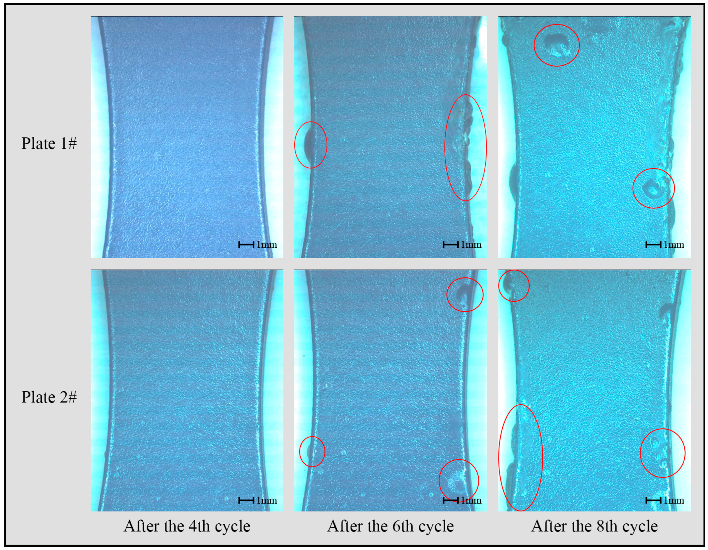
After each test period, the macroscopic morphology of two specimens was recorded. The focal point of the observation was the working section in the middle of the specimens. The macro-morphology images of Plate 1# and Plate 2# at critical time points, which were the end of the 4th, 6th, 8th cycles, were collected and integrated in Figure 3. At each critical time point, new emerging bulge or corrosion products were marked with red circles in Figure 3. It can be observed that the locations of the bubbling of the two specimens were different due to the instability of coating preparation. And most of the bubble appeared at the edge of the specimens, which suggested that the weak areas of the coating were at the edge of the specimens. From the zeroth cycle to the fourth cycle, the coating surface of specimens was still relatively complete. After the fifth cycle, there appeared micro porous in Plate 2#, but Plate 1# was still in good condition. However, after the sixth cycle, a small bubbling defect was observed in the working section of Plate 1#, and the size of bubbling defects of Plate 2# were bigger than before. From the seventh cycle to the eighth cycle, the number of the bubbles increased and the size of these bubbling defect grew in both specimens.
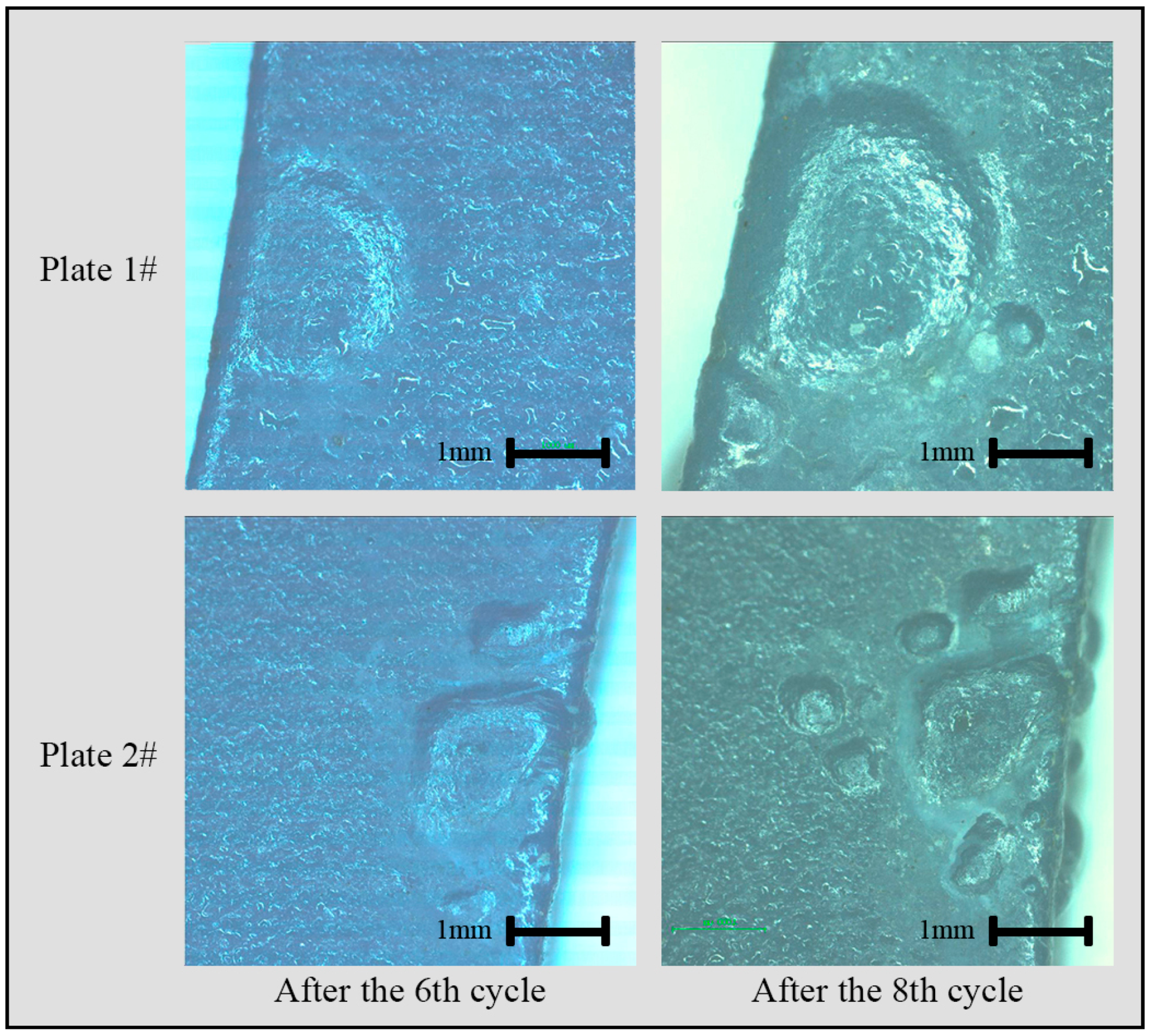
The micro-morphology images of Plate 1# and Plate 2# at the end of the 6th and 8th cycles were also recorded and integrated in Figure 4. After the 6th cycle, the bubbling defects of Plate 1# was inconspicuous and that of Plate 2# was small. After the 8th cycle, the size of the bubbles of Plate 1# was significantly bigger than before, and the number of the bubbles of Plate 2# increased and the range was larger.
3.2. Analysis of the Electrochemical Impedance Data
Electrochemical impedance spectroscopy has been in use widely in a semi-quantitative way to evaluate and predict the service life of protective coatings. The electrochemical impedance data of Plate 1# and Plate 2# were measured at the end of each cycle. It can be seen obviously in Figure 5 that the impedance data of each cycle were equally spaced on a logarithmic scale for a total of 50 points. After the first cycle, the impedance modulus of the two specimens displayed very high value (>109 Ω·cm2) at 0.1 Hz, which suggested that the coating can still protect the metal from corrosive action. Nevertheless, after the second cycle, the impedance modulus values |Z| at the low-frequency of both specimens declined sharply to about 106 Ω·cm2. In this stage, the barrier ability of the coating to water and other particles had been very low. After the third cycle, the order of the impedance at 0.1 Hz was approximately 105 Ω·cm2, which meant the electrochemical corrosion reaction had occurred at the interface between coating and metal. After the fourth cycle, the coating impedance increased slightly which reflected the self-healing behavior of the coating. The mechanism of the self-healing behavior is that corrosion products jammed the pores of the coating, obstructing the medium infiltration [27]. From the fifth cycle to the eighth cycle, low-frequency impedance value was in the range of 104–105 Ω·cm2, indicating that the protective performance of the coating had been very weak.
4. Life Prediction
4.1. The Brief of Theoretical Life Prediction Model
At present, there are few studies on the prediction of coating service life. Mayne [28] proposed a coating life prediction formula (Equation (1)) based on the theory of coating polarization resistance control, combining Fick’s Law of Diffusion with Electrochemical Studies on Coated Steel Plates:
where L is the coating life; l is the thickness of the coating; D is the diffusion coefficient of the coated ions; φ is a constant; ps is the adhesion of the coating; σm is the pressure applied to the steel surface.
Chuang et al. [29] established a mathematical model based on coating bubbling (Equation (2)). The bulge growth rate V is regarded as a function of moment, material properties and temperature:σ
where σf is the stratified stress; W is the cross-sectional area of the coating; Dbδb is the interfacial diffusion rate; Ω, k, T are constants; E and V are the elastic modulus and the Poisson’s ratio of the coating in the wet state, respectively; h is the total coating thickness.
In addition, some Chinese scholars have proposed a life prediction formula based on corrosive media penetration [30]:
where q is the infiltration amount of the medium after infinite length of time; Q is the infiltration of the medium to the organic matter after infinite length of time; x is the coating thickness; A and B are proportional coefficients; D is the diffusion coefficient; t is the time that the media penetrates through the organic coating, which is regarded as the service life of the coating.
Geng et al. [31] introduced the gray theory into the failure study of the anti-corrosion coating of the bridge, and constructed the GM (1, 1) model with the area variation of the coating corrosion pits. And based on this, the general prediction formula of corrosion ressitance coating life of bridge is deduced by the following formula.
Lin [32] proposed a new life formula based on the research of Geng et al. He assumed that the change in the corrosive area of the coating is developed exponentially, resulting in the protective life of the coating as follows:
where A and B are constants; S is the corrosion area; N is the equidistant distance; t0 is the initial time.
Although the above studies established certain specific formulas for coating life, their accuracy is questionable. Due to the diversity of the coating type and the difference in the corrosive environment, the effective formula for accurately predicting the service life of the coating has not been found so far.
4.2. Prediction from |Z| Data at Low Frequency
As Lee and Mansfield [18] have proposed, polymer coating quality can be classified into three stages, which are defined as ‘good’, ‘intermediate’ and ‘poor’. For the ‘good’ coating of which the thickness is range from 50 μm to 250 μm, the impedance modulus values in 0.1 Hz are greater than 109 Ω·cm2 and the plots approximate a tilt straight line, while for the ‘intermediate’ coating the data curves maintain a level of straight for a short distance then decline sharply, and the impedance modulus values in 0.1 Hz are in the range of 106–108 Ω·cm2. For the ‘poor’ coating the data is about 106 Ω·cm2. Based on the |Z| data at low frequency, the service life of coatings can be predicted approximately. According to this method, the failure criterion of coatings can be expressed by Equation (7).
where |Z(t)|lowfreq is the coating impedance at low frequency corresponding to the aging time t; |Z|poor is the coating impedance corresponding to the ‘poor’ stage at low frequency. In addition, Cai et al. [21] also proposed a failure criterion, which is similar to Equation (7):
For Plate 1# and Plate 2#, the failure criterion can be written by Equation (2). So it can be easily obtained that the failure cycle of both specimens is the 3th cycle by |Z| data at 0.01 Hz.
However, according to the analysis of morphology in Section 3.1, in the 3rd cycle, the coating of the two specimens was still in good condition. Hence, it is not accurate enough to predict the coating lifetime by using impedance at low frequency.
4.3. Degradation Kinetics Model
Bierwagen et al. [7] proposed that the low-frequency impedance is very sensitive to the coating degradation process, and the impedance of the coating at low frequency is in accordance with Equations (9) and (10).
where t is coating aging time; |Z|t and |Z|0 is the coating impedance magnitude at 0.1 Hz corresponding to the aging time t and 0, respectively; |Z|m is the impedance of metal substrates and θ is reaction constant. The smaller the θ in the same environment, the more sensitive the coating is to the environment, which means that the more easily the coating is corroded. Based on the experimental data, θ was fitted to obtain the degradation kinetics equation of the coating in the specific environment. The life of the coating can be predicted from the degradation equation:
where Tfail is the failure time, and |Z|fail is the failure modulus of the coating.
According to the experimental results, the impedance data at 0.1 Hz of Plate 1# and Plate 2# were fitted with the degradation kinetic model using Equation (4). The fitting result is shown in Figure 6. It can be seen from the figure, the fitting lines of the two specimens almost coincides, because the two groups of test data are similar.
Then, the forecast cycles of Plate 1# and Plate 2# were predicted by the aging slash obtained by the fitting of Plate 2# and Plate 1# data, respectively. However, the results solved by the linear fitting are not integers. The final forecast cycles can be gotten by rounding the computational forecast cycles. And negative results were considered as invalid prediction. The prediction results are shown in Table 1. As can be seen from Table 1, the maximum prediction error of both specimens is 3 cycles corresponding to the 3rd cycle, and others are less than 2 cycles. The average error of the effective prediction is 1.36.
The failure impedance modulus of Plate1# and Plate 2# can be taken as 106 Ω·cm2. Hence, the failure cycle of the specimens can be obtained by Equation (5), and the results is the 4th cycle, which is one cycle later than the forecast cycle judged by |Z| data at low frequency in Section 4.2.
However, in the process of using the degradation kinetics model, the experimental data were not fully utilized and there is a relatively large error in the cycle prediction. This method as coating failure criterion needs to be further improved.
4.4. Improved Degradation Kinetics Model
It was found that the degradation kinetics model is not suitable for the case when the damage of the coating is serious. In addition, only a single frequency impedance is adopted in the degradation kinetics model, so the accidental error is relatively large. Based on the experimental results, the influence of the matrix impedance on the impedance of the coating is negligible and impedances at different frequencies are sensitive to the corrosion process more or less. Hence, different degradation equations can be obtained by the |Z|t, |Z|0 at different frequencies.
According to the above-mentioned viewpoints, with the help of the degradation kinetics model, it can be proposed that the impedance magnitude accords with Equation (12):
where Zt, T and Z0 are column vectors, and the elements of these vectors are denoted by Zti, Ti and Z0i. Among them, Zti and Z0i are the fitting results of lg|Z|t and lg|Z|0 at frequency fi, respectively. A is a diagonal matrix and the diagonal elements Aii are the fitting results given by Equation (13).
After getting the diagonal matrix A, the time vector T can be solved by Equation (14) using experimental data |Z|t of the specimen to be predicted. The prediction period Tp satisfies the minimum mean square error:
If the coating failure impedance at each frequency Tfi is known, a failure time vector Tf can be solved by Equation (15). The final predicted failure time can be obtained by finding the minimum mean square error of Tfi, which is the same as solving the Tp.
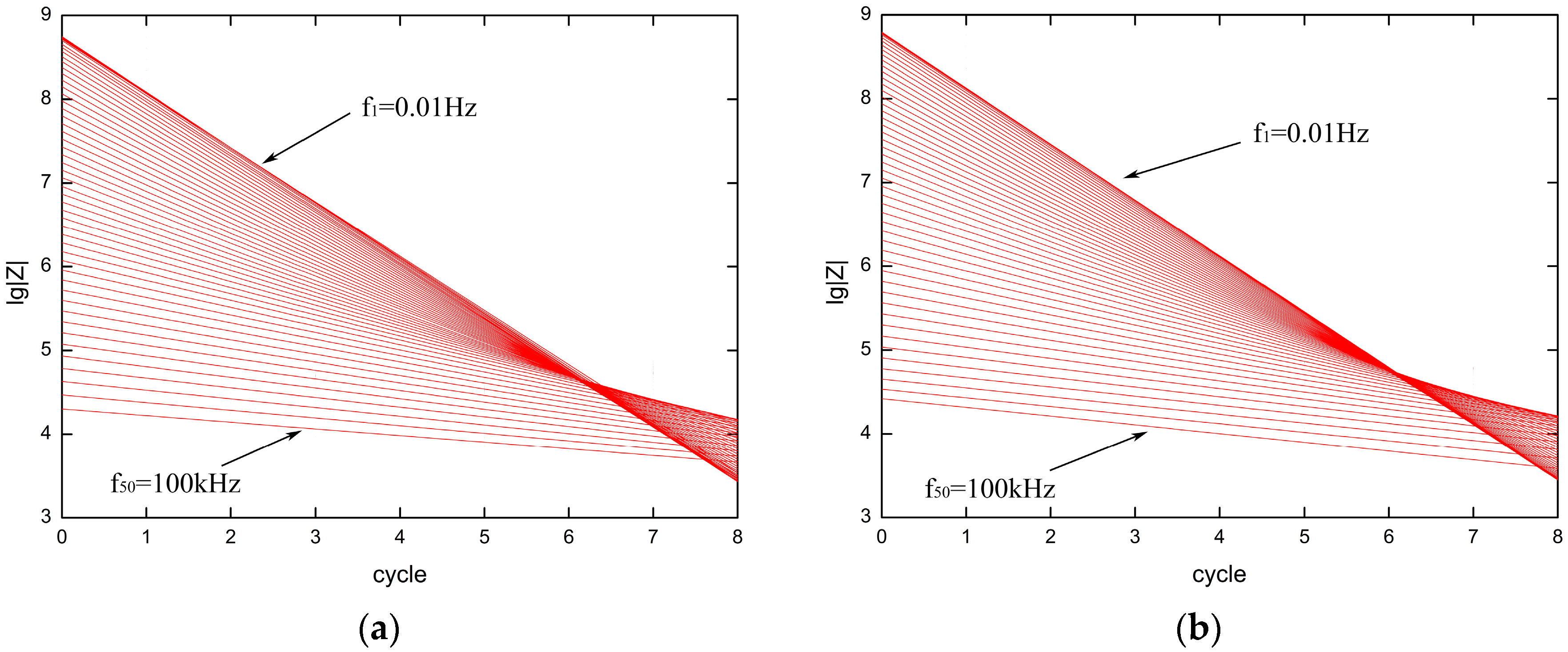
Then, the cross validation method is used to apply this model to the experimental data. The fitting straight lines of Plate 1# and Plate 2# at multiple frequencies gotten by Equation (7) are shown in Figure 7. The selection range of frequency points is from 0.01 Hz to 100,000 Hz, of which the total number is 49. It can be seen from the figure that as the frequency increases, the slope of the fitting line decreases, which illustrates that in the corrosion process, the higher the frequency is, the smaller the change in the measured impedance modulus is.
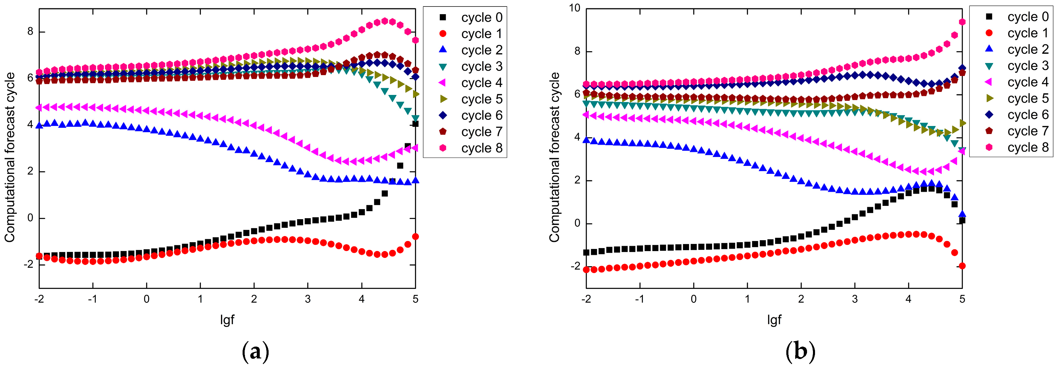
The results of the prediction time at each frequency Ti obtained by Equation (15) is shown in Figure 8. The predicted values of each cycle at low frequency are relatively stable, while the predicted values at high frequency have a large deviation. It may be due to the fact that the impedance values at high frequencies are more sensitive to the coating degradation than that at low frequencies, which plays a role in correcting the calculation of the final forecast results.
Finally, the prediction cycles of improved degradation kinetics model obtained by Equation (14) are listed in Table 2. The final forecast cycles were also obtained by rounding the computational forecast cycles and negative results were considered as invalid prediction. The average error of the effective prediction is 0.87, of which the accuracy is increased by about 36% compared to the average error of traditional degradation kinetics model.
The low-frequency failure impedance of the coating is about 106 Ω·cm2, but there is no basis for the determination of the non-low-frequency failure impedance. Therefore, the failure cycle can be predicted by the experimental data at the frequencies range from 0.01 Hz to 1 Hz. The final results are the 4th cycle, which is the same as the failure cycle of traditional degradation kinetics model.
Compared with the traditional degradation kinetics model, the improved model performs better in predicting cycles. However, the coating was still judged prematurely to be ineffective. According to the analysis of morphology in Section 3.1, the true failure cycle of the two specimens should be the 5th cycle. What is more, this improved model fails to reflect the detail of the coating degradation process.
4.5. Neural Network Classification Model Based on Sample Detection
Specific artificial networks and impedance spectrum analysis were combined to establish the neural network classification model. This model applies Kohonen neural networks to analyze the impedance spectrum directly, which avoids the choice of equivalent circuit. The topology structure of the SOM adopted to predict the service life of the coating is showed in Figure 9. The network consists of two layers of neurons ordered in a low-dimensional map, a linear array of artificial neurons. In the second layer, three neurons represent the three stages of the coating degradation process [18], of which corresponding impedance at low frequency and characteristics are shown in Figure 10. In the first stage, the coating has good protective properties and has little change compared with the state before corrosion; in the second stage, there appears micro porous and small bubbling defect and it tends to peel off in coatings; and in the third stage, coating shows big flaws and is completely ineffective.
The essence of the SOM network is that neurons in the competition layer compete with each other in order to get an opportunity to respond to the input sample. The result of the competition is that only one neuron can become the winner, which responds to the corresponding input according to its weight. In the process of competition, the adjustment of weights is based on the input sample, so the role of the sample is important. We can set up a mechanism to select excellent samples automatically, and remove some noise samples. In this way, the weight adjustment is better.
Therefore, the dispersion criterion is used to improve the training of neural networks. In the feature space, the classification is easier to implement while the intra-class pattern distribution is dense and the distance between the different model features is far away. Dispersion is a criterion function that can reflect the distance between classes and interclass distances. In the process of network competition, screening samples can dynamically reduce the dispersion within the group to improve the final recognition of the network performance. The process of predicting the experimental data period using the neural network model based on sample detection is divided into four steps as follows.
Step 1: Build the SOM-A network. Train the network through sample input. After the training, the basic classification of the samples can be judged based on the winning neurons. During the training process, each input data xs is presented to the neural network. Only the neuron whose weight vector is most similar to the input vector xs is stimulated and this process is so called competitive learning. In more mathematical terms, the winning neuron stimulated by the input is selected as the one providing the minimal Euclidean distance to the xs:
where xsi and ωji are the ith coordinate of the input data xs and the ith weight of neuron j in the second layer, respectively. After the winning neuron is selected, the weights ωji of each neuron j are updated on the basis of the difference between their old value and the magnitude of the input data xsi. This correction is scaled according to the distance from the winner dr.
where η is the learning rate; ωij(t) is the numerical value of the weight ωij at the previous iteration. The size of dmax, which at the beginning of learning covers the whole neural network, decreases during the training process and finally the value is zero. The learning rate η is one of important parameters and is also changing during the training by Equation (18):
where ηinitial and ηfinal are the initial value and the final value of the learning rate constant η, respectively; nprevious and ntotal are the previous iteration and the entire number of the iteration, respectively. When the neural network training is completed, the data to be predicted will be input to the network, then the corresponding classification results can be obtained, which is so called network testing.
Comparing the Euclidean distance between the test data and the training data. In the classifying step, the Euclidean distance corresponding to the neuron stimulated by the test data is obtained from the neural network. The Euclidean distances of each set of training data are also obtained. The training data with the shortest distance from the test data will be the winner, of which the corresponding period is the forecast period of the test data.
Step 2: Calculate the average mi of each class sample according to the classification results. The dispersion of each sample with mi can be obtained using Equation (19).
Step 3: Determine the distance threshold according to the dispersion and select the sample within the distance to obtain a set of samples with smaller dispersion value.
Step 4: Build the SOM-B network. Train the network through the selected sample input. The process is the same as the first step.
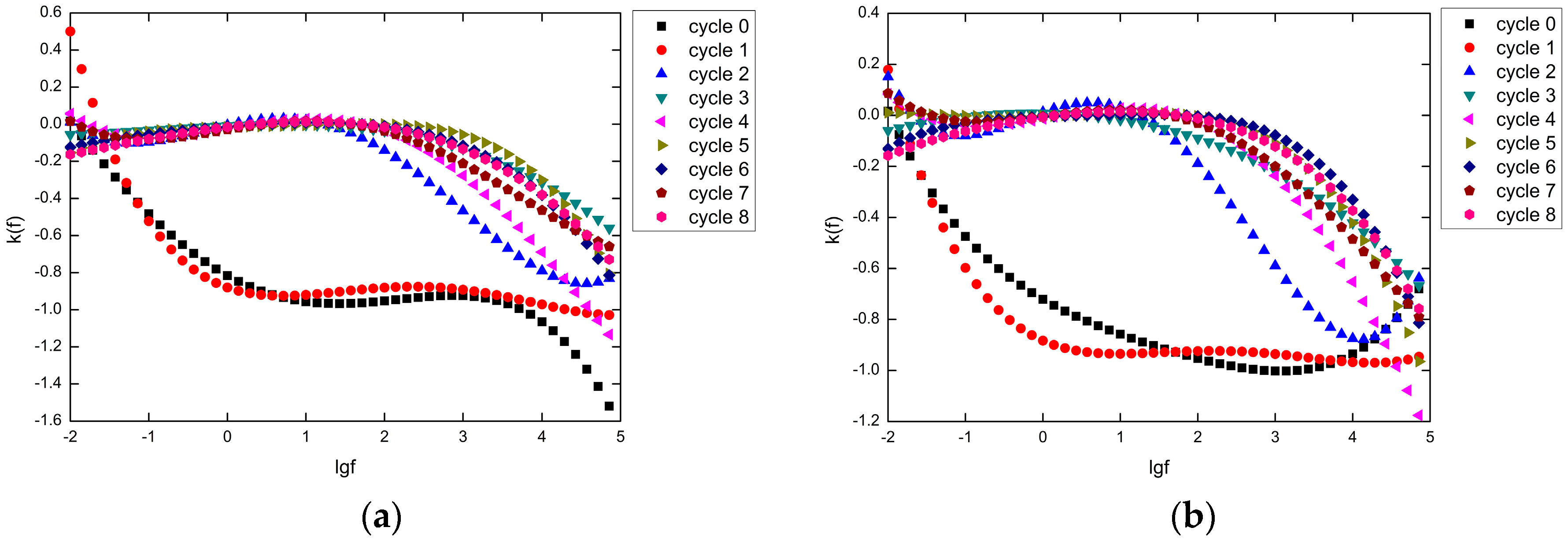
Compared with other EIS parameters, the changing rate in impedance which satisfies Equation (20) can reflect the changing process of the impedance more sensitively in the entire frequency range and can help to recognize the features of deterioration process more clearly. The changing rate in impedance expressed in differential form can probably intensify the characteristics of each stage in the frequency range. So the changing rate of impedance of each cycle can be took as an input sample for network training. Therefore, for the classification purpose, the failure stages of the coating can be distinguished effectively which does not require to build EC (Equivalent Circuit) and analyze other parameters.
Actually, in practical applications, the changing rate k can be applied in the discrete form as given by Equation (21).
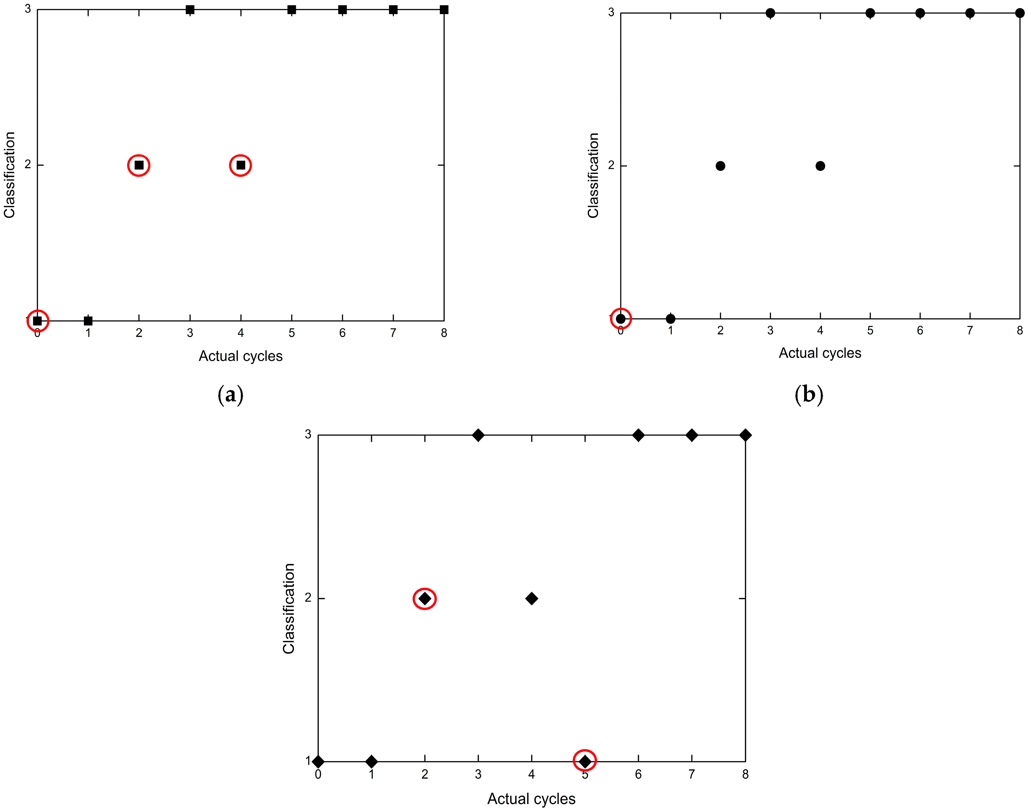
In the following, the process and results of applying the neural network model to analyze the impedance data of Plate 1#, 2# and 3# will be described. There are some erroneous experimental data in the Plate 3# data, which are introduced here to verify the validity of the sample detection. It took the changing rate in impedance as the input sample of the Kohonen network, and the parameters k of these three plates are shown in Figure 11. The classification results of the specimens are shown in Figure 12. It is obvious that the cycle classification results of Plate 1# is the same as that of Plate 2#. It appears jump phenomenon in the 4th cycle because of self-healing behavior occurring when corrosion happens. Corrosion products jammed the pores of the coating, obstructing the medium infiltration [27]. During the sample detection process, the data in the red circle are deleted. It is obvious that the data at the fifth cycle of Plate #3 is included, which is caused by the experimental measurement error.
The cross-validation is also used in here. The cycle forecast of Plate 1# was obtained using the network trained by the impedance data of Plate 2#, and the cycle forecast of Plate 2# was gotten by the network trained by the data of Plate 1#. The Euclidean distance between the cycles of testing sample and the training sample was calculated, and the cycle of training sample whose Euclidean distance with the predicted cycle was minimum was selected as the forecast cycle of the test cycle.
The final cycle prediction results are incorporated into Table 3. Compared with the previous two models, the prediction cycle error of the neural networks model is greatly reduced. Most of the forecast cycles are the same as the corresponding real cycles. The average error is 0.22, and the accuracy is increased by about 84% compared to the traditional degradation kinetics model and 75% compared to the improved degradation kinetics model. The reason why the errors of the two degradation kinetics models are large is that they cannot reflect the process of coating self-healing behavior. However, the classification results of SOM is a perfect simulation of this phenomenon.
For the determination of the failure cycle, it can be considered that the third stage of coating corrosion is the failure stage. So the failure cycle of the two specimens is the 5th cycle according to the classification results of SOM, which is in agreement with the results of morphological analysis. As can be seen from Table 4, the failure criterion of neural network model is the best.
5. Conclusions
Applicability of the improved degradation kinetics model and the neural network classification model in life prediction of coatings is discussed. Compared with the degradation kinetics model, the improved degradation kinetics model ignores the influence caused by the impedance of the matrix and applies multi-frequency impedance of specimens in order to reduce the accidental error. As a result, the prediction accuracy can be improved by 36%, approximately.
The neural network classification model not only avoids the problem that the equivalent circuit is difficult to select, but also takes into account the change of impedance modulus and impedance at multiple frequencies. The prediction cycle error is significantly reduced compared to the other two models. The classification results reflect the coating self-healing behavior accurately and the failure cycle judged by neural network model coincides with the results of morphological analysis.
Acknowledgments
This research was supported by the National High Technology Research and Development Program of China (863 Program), the Aeronautical Science Foundation of China (No.: 2014ZE21009) and the Foundation of key laboratory of Beijing, China.
Author Contributions
Yuanming Xu and Junshuang Ran conceived and designed the experiments; Wei Dai and Weifang Zhang performed the experiments; Junshuang Ran and Wei Dai analyzed the data; Yuanming Xu contributed analysis tools; Yuanming Xu and Junshuang Ran wrote the paper.
Conflicts of Interest
The authors declare no conflict of interest.
References
- Croll, S.G.; Hinderliter, B.R.; Liu, S. Statistical approaches for predicting weathering degradation and service life. Prog. Org. Coat. 2006, 55, 75–87. [Google Scholar] [CrossRef]
- Zhang, J.T.; Hu, J.M.; Zhang, J.Q.; Cao, C.N. Studies of impedance models and water transport behaviors of polypropylene coated metals in NaCl solution. Prog. Org. Coat. 2004, 49, 293–301. [Google Scholar] [CrossRef]
- Shreepathi, S.; Guin, A.K.; Naik, S.M.; Vattipalli, M.R. Service life prediction of organic coatings: Electrochemical impedance spectroscopy vs actual service life. J. Coat. Technol. Res. 2011, 8, 191–200. [Google Scholar] [CrossRef]
- Nguyen, A.S.; Musiani, M.; Orazem, M.E.; Pebere, N.; Tribollet, B.; Vivier, V. Impedance study of the influence of chromates on the properties of waterborne coatings deposited on 2024 aluminium alloy. Corros. Sci. 2016, 109, 174–181. [Google Scholar] [CrossRef]
- Cao, C.N.; Zhang, J.Q. An Introduction to Electrochemical Impedance Spectroscopy; Science Press: Beijing, China, 2003. [Google Scholar]
- Scully, J.R.; Silverman, D.C.; Kendig, M.W. Electrochemical Impedance: Analysis and Interpretation, ASTM STP 1188; American Society for Testing and Materials: Philadelphia, PA, USA, 1993. [Google Scholar]
- Bierwagen, G.; Tallman, D.; Li, J.P.; He, L.Y.; Jeffcoate, C. EIS studies of coated metals in accelerated exposure. Prog. Org. Coat. 2003, 46, 148–157. [Google Scholar] [CrossRef]
- Zhang, J.Q.; Sun, G.Q.; Cao, C.N. EIS data analysis for evaluation of protective property of organic coatings. Corros. Sci. Prot. Technol. 1994, 6, 318–325. [Google Scholar]
- Zubielewicz, M.; Gnot, W. Mechanisms of non-toxic anticorrosive pigments in organic waterborne coatings. Prog. Org. Coat. 2004, 49, 358–371. [Google Scholar] [CrossRef]
- Mahdavian, M.; Attar, M.M. Investigation on zinc phosphate effectiveness at different pigment volume concentrations via electrochemical impedance spectroscopy. Electrochim. Acta 2005, 50, 4645–4648. [Google Scholar] [CrossRef]
- Amirudin, A.; Thieny, D. Application of electrochemical impedance spectroscopy to study the degradation of polymer-coated metals. Prog. Org. Coat. 1995, 26, 1–28. [Google Scholar] [CrossRef]
- Zuo, Y.; Pang, R.; Li, W.; Xiong, J.P.; Tang, Y.M. The evaluation of coating performance by the variations of phase angles in middle and high frequency domains of EIS. Corros. Sci. 2008, 50, 3322–3328. [Google Scholar] [CrossRef]
- Mahdavian, M.; Attar, M.M. Another approach in analysis of paint coatings with EIS measurement: Phase angle at high frequencies. Corros. Sci. 2006, 48, 4152–4157. [Google Scholar] [CrossRef]
- Mansfeld, F.; Tsai, C.H. Determination of coating deterioration with EIS: I. Basic relationships. Corrosion 1991, 47, 958–963. [Google Scholar] [CrossRef]
- Fernandez-Perez, B.M.; Gonzalez-Guzman, J.A.; Gonzalez, S.; Souto, R.M. Electrochemical impedance spectroscopy investigation of the corrosion resistance of a waterborne acrylic coating containing active electrochemical pigments for the protection of carbon steel. Int. J. Electrochem. Sci. 2014, 9, 2067–2079. [Google Scholar]
- Zhu, Y.F.; Xiong, J.P.; Tang, Y.M.; Zuo, Y. EIS study on failure process of two polyurethane composite coatings. Prog. Org. Coat. 2010, 69, 7–11. [Google Scholar] [CrossRef]
- Cai, J.P.; Sun, Z.H.; Cui, J.H. Establishment of degradation dynamic model for organic coatings. Mater. Prot. 2012, 45, 8–10. [Google Scholar]
- Lee, C.C.; Mansfeld, F. Automatic classification of polymer coating quality using artificial neural networks. Corros. Sci. 1998, 41, 439–461. [Google Scholar] [CrossRef]
- Zhao, X.; Wang, J.; Kong, T.; Zhang, W.; Wang, Y.H. Investigation of deterioration process of organic coating using 1-dimention SOM network combined with EIS. Corros. Sci. Prot. Technol. 2008, 20, 275–278. [Google Scholar]
- Zhen, F. Simple talk about the forecast theory about coating’s life. Coat. Appl. Electr. Plat. 2005, 3, 3–5. [Google Scholar]
- Cai, J.P.; Liu, M.; An, Y.H. Degradation kinetics of protective coating for aluminum alloy. J. Chin. Soc. Corros. Prot. 2012, 32, 256–261. [Google Scholar]
- Evans, M. A statistical degradation model for the service life prediction of aircraft coatings: With a comparison to an existing methodology. Polym. Test. 2012, 31, 46–55. [Google Scholar] [CrossRef]
- Wnag, H.T.; Han, E.H.; Ke, W. Predictive model for atmospheric corrosion of aluminium alloy by artificial neural network. J. Chin. Soc. Corros. Prot. 2006, 26, 272–276. [Google Scholar]
- Akbarinezhad, E.; Bahremandi, M.; Faridi, H.R.; Rezaei, F. Another approach for ranking and evaluating organic paint coatings via electrochemical impedance spectroscopy. Corros. Sci. 2009, 51, 356–363. [Google Scholar] [CrossRef]
- Krahmer, D.M.; Polvorosa, R.; de Lacalle, L.N.L.; Alonso-Pinillos, U.; Abate, G.; Riu, F. Alternatives for specimen manufacturing in tensile testing of steel plates. Exp. Tech. 2016, 40, 1555–1565. [Google Scholar] [CrossRef]
- Rodríguez-Barrero, S.; Fernández-Larrinoa, J.; Azkona, I.; López de Lacalle, L.N.; Polvorosa, R. Enhanced performance of nanostructured coatings for drilling by droplet elimination. Mater. Manuf. Process. 2016, 31, 593–602. [Google Scholar] [CrossRef]
- Zhao, X. Characteristics of Electrochemical Impedance Spectroscopy in Deterioration Process of Organic Coating. Ph.D. Thesis, Ocean University of China, Qingdao, China, 2007. [Google Scholar]
- Cmaitland, C.; Mayne, J.E.O. Factors affecting the electrolytic resistance of polymer films. Off. Dig. 1962, 34, 972. [Google Scholar]
- Fu, D.X.; Xu, B.S.; Zhang, W. Research progress on microscopic mechanism of foaming of organic coatings. J. Mater. Prot. 2007, 40, 42–45. [Google Scholar]
- Ren, B.N. Corrosion and Protection of Highway Steel Bridge; China Communications Press: Beijing, China, 2002. [Google Scholar]
- Geng, G.Q.; Lin, J.; Liu, L.J.; Cui, J.N. Life prediction system for protective coating of steel bridge. J. Chang’an Univ. (Nat. Sci. Ed.) 2006, 26, 43–47. [Google Scholar]
- Lin, J. Study on Protection, Failure Law and Life Prediction of Corrosion Protective Coatings for Bridge Steel Structures. Master’s Thesis, Chang’an University, Xi’an, China, 2006. [Google Scholar]
Figure 1.
Pattern of specimens (units: mm).

Figure 2.
Acceleration test process.
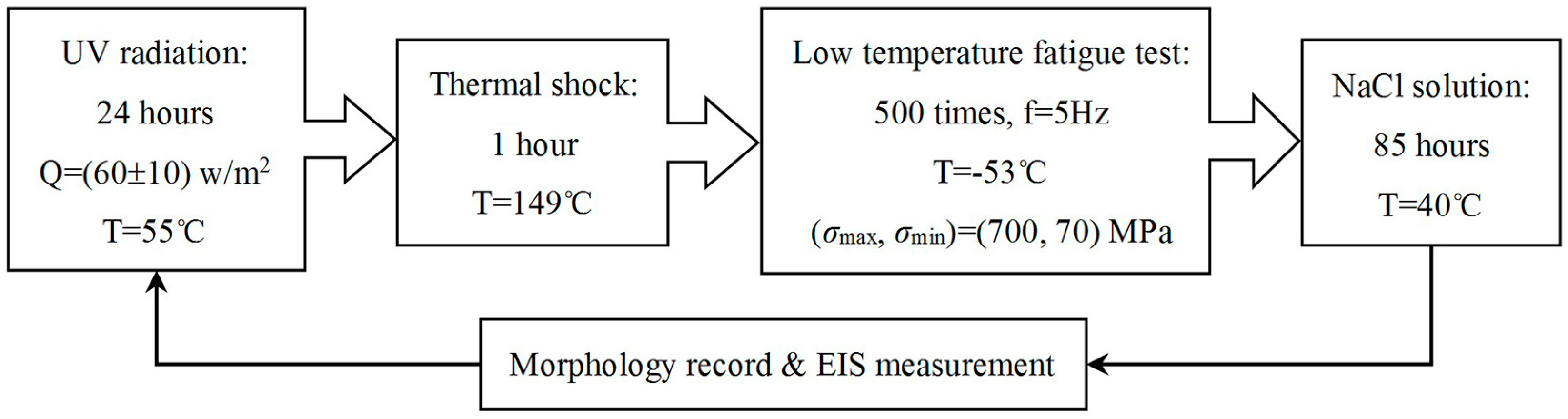
Figure 3.
Macro-morphology of the specimens.

Figure 4.
Micro-morphology of the specimens.

Figure 5.
Impedance modulus spectrums of the specimens: (a) Plate 1#; (b) Plate 2#.
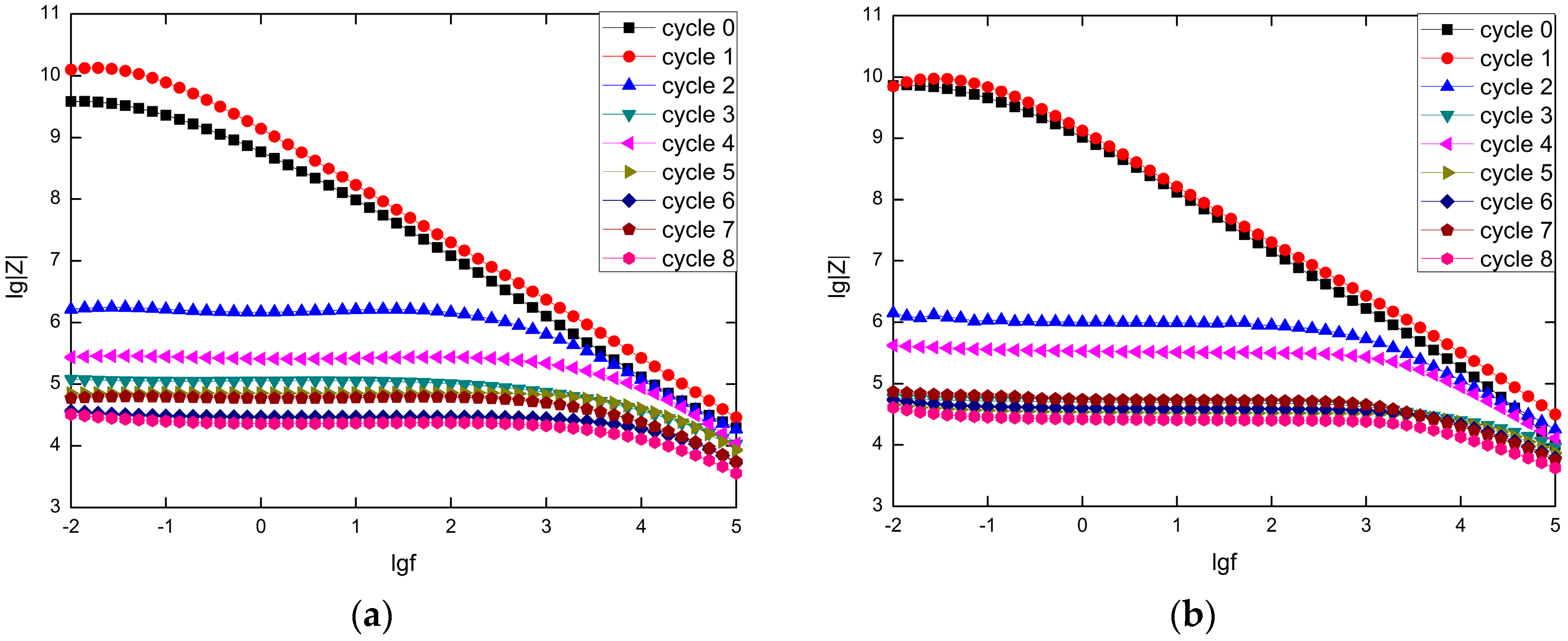
Figure 6.
The fitting results of the two specimens using degradation kinetic model: (a) Plate 1#; (b) Plate 2#.
Figure 6.
The fitting results of the two specimens using degradation kinetic model: (a) Plate 1#; (b) Plate 2#.
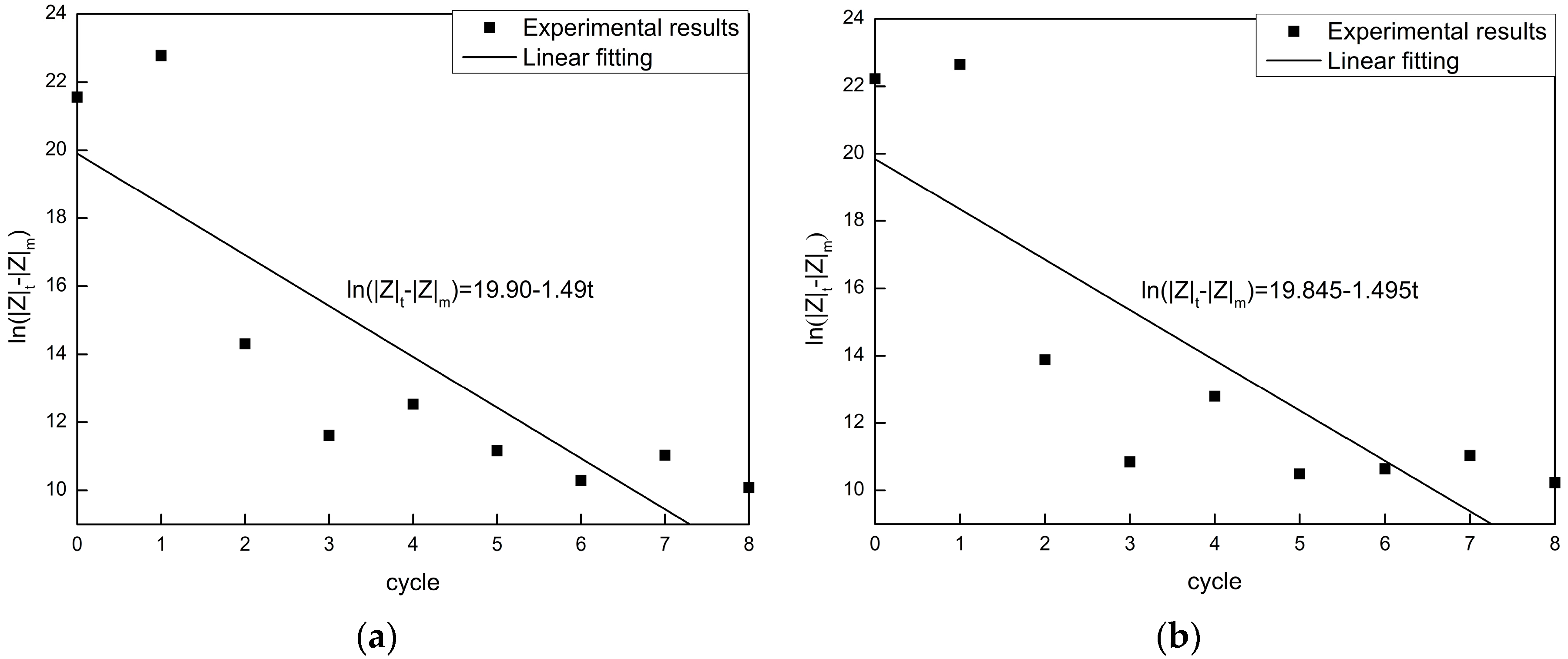
Figure 7.
The fitting results of the two specimens using improved degradation kinetic model: (a) Plate 1#; (b) Plate 2#.
Figure 7.
The fitting results of the two specimens using improved degradation kinetic model: (a) Plate 1#; (b) Plate 2#.

Figure 8.
Results of Ti: (a) Plate 1#; (b) Plate 2#.

Figure 9.
The topology structure of the self-organizing feature mapping network (SOM).
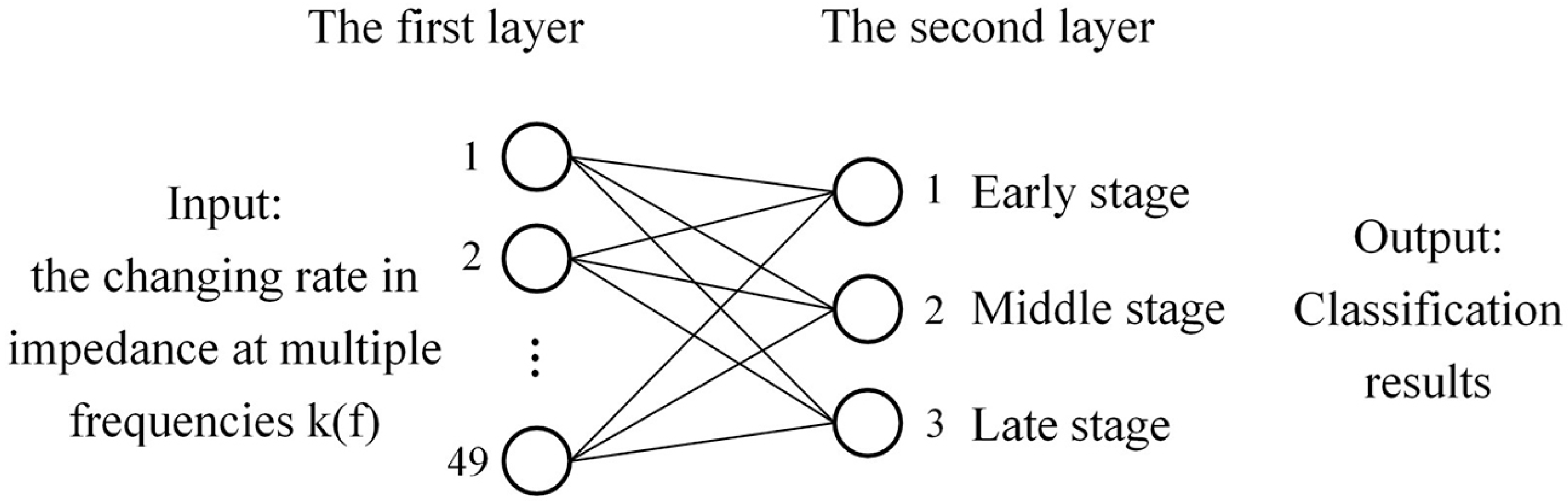
Figure 10.
The three stages of coating corrosion process.
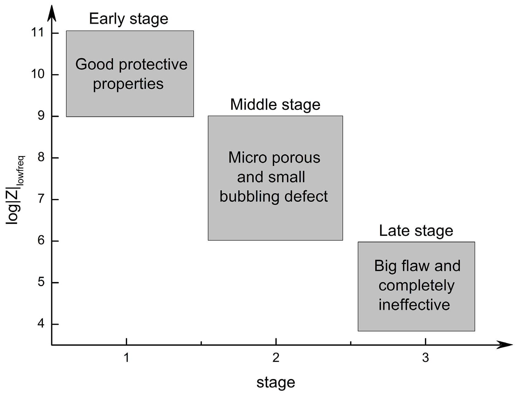
Figure 11.
The changing rate in impedance k: (a) Plate 1#; (b) Plate 2#; (c) Plate 3#.


Figure 12.
The classification results: (a) Plate 1#; (b) Plate 2#; (c) Plate 3#.

Table 1.
Prediction results of degradation kinetics model.
| Real Cycle | Plate 1# | Plate 2# | ||||
|---|---|---|---|---|---|---|
| Computational Forecast Cycle | Rounding Forecast Cycle | Prediction Cycle Error | Computational Forecast Cycle | Rounding Forecast Cycle | Prediction Cycle Error | |
| 0 | −1.56 | / | / | −1.15 | / | / |
| 1 | −1.85 | / | / | −1.96 | / | / |
| 2 | 4.04 | 4 | 2 | 3.70 | 4 | 2 |
| 3 | 6.08 | 6 | 3 | 5.51 | 6 | 3 |
| 4 | 4.77 | 5 | 1 | 4.89 | 5 | 1 |
| 5 | 6.32 | 6 | 1 | 5.81 | 6 | 1 |
| 6 | 6.22 | 6 | 0 | 6.39 | 6 | 0 |
| 7 | 5.95 | 6 | 1 | 5.90 | 6 | 1 |
| 8 | 6.49 | 6 | 2 | 6.53 | 7 | 1 |
Table 2.
Prediction results of improved degradation kinetics model.
| Real Cycle | Plate 1# | Plate 2# | ||||
|---|---|---|---|---|---|---|
| Computational Forecast Cycle | Rounding Forecast Cycle | Prediction Cycle Error | Computational Forecast Cycle | Rounding Forecast Cycle | Prediction Cycle Error | |
| 0 | −0.52 | / | / | −0.31 | 0 | 0 |
| 1 | −1.36 | / | / | −1.34 | / | / |
| 2 | 2.90 | 3 | 1 | 2.52 | 3 | 1 |
| 3 | 6.03 | 6 | 3 | 5.15 | 5 | 2 |
| 4 | 3.88 | 4 | 0 | 4.00 | 4 | 0 |
| 5 | 6.39 | 6 | 1 | 5.42 | 5 | 0 |
| 6 | 6.38 | 6 | 0 | 6.59 | 7 | 1 |
| 7 | 6.21 | 6 | 1 | 5.96 | 6 | 1 |
| 8 | 7.04 | 7 | 1 | 7.07 | 7 | 1 |
Table 3.
Prediction results of neural network model.
| Real Cycle | Plate 1# | Plate 2# | ||
|---|---|---|---|---|
| Forecast Cycle | Prediction Cycle Error | Forecast Cycle | Prediction Cycle Error | |
| 0 | 0 | 0 | 0 | 0 |
| 1 | 1 | 0 | 1 | 0 |
| 2 | 2 | 0 | 2 | 0 |
| 3 | 3 | 0 | 3 | 0 |
| 4 | 4 | 0 | 4 | 0 |
| 5 | 6 | 1 | 6 | 1 |
| 6 | 5 | 1 | 5 | 1 |
| 7 | 7 | 0 | 7 | 0 |
| 8 | 8 | 0 | 8 | 0 |
Table 4.
The failure cycle determined by different analytical methods and models.
| Analytical Methods or Models | The Failure Cycle |
|---|---|
| Morphological analysis | 5 |
| Analysis of |Z| data at low frequency | 3 |
| Degradation kinetics model | 4 |
| Improved degradation kinetics model | 4 |
| Neural network model | 5 |
© 2017 by the authors. Licensee MDPI, Basel, Switzerland. This article is an open access article distributed under the terms and conditions of the Creative Commons Attribution (CC BY) license (http://creativecommons.org/licenses/by/4.0/).
Share and Cite
MDPI and ACS Style
Xu, Y.; Ran, J.; Dai, W.; Zhang, W. Investigation of Service Life Prediction Models for Metallic Organic Coatings Using Full-Range Frequency EIS Data. Metals 2017, 7, 274. https://doi.org/10.3390/met7070274
AMA Style
Xu Y, Ran J, Dai W, Zhang W. Investigation of Service Life Prediction Models for Metallic Organic Coatings Using Full-Range Frequency EIS Data. Metals. 2017; 7(7):274. https://doi.org/10.3390/met7070274
Chicago/Turabian StyleXu, Yuanming, Junshuang Ran, Wei Dai, and Weifang Zhang. 2017. "Investigation of Service Life Prediction Models for Metallic Organic Coatings Using Full-Range Frequency EIS Data" Metals 7, no. 7: 274. https://doi.org/10.3390/met7070274
Note that from the first issue of 2016, this journal uses article numbers instead of page numbers. See further details here.