Effect of Structural Heterogeneity of 17Mn1Si Steel on the Temperature Dependence of Impact Deformation and Fracture

 , ,
, ,  and
and
Abstract
:1. Introduction
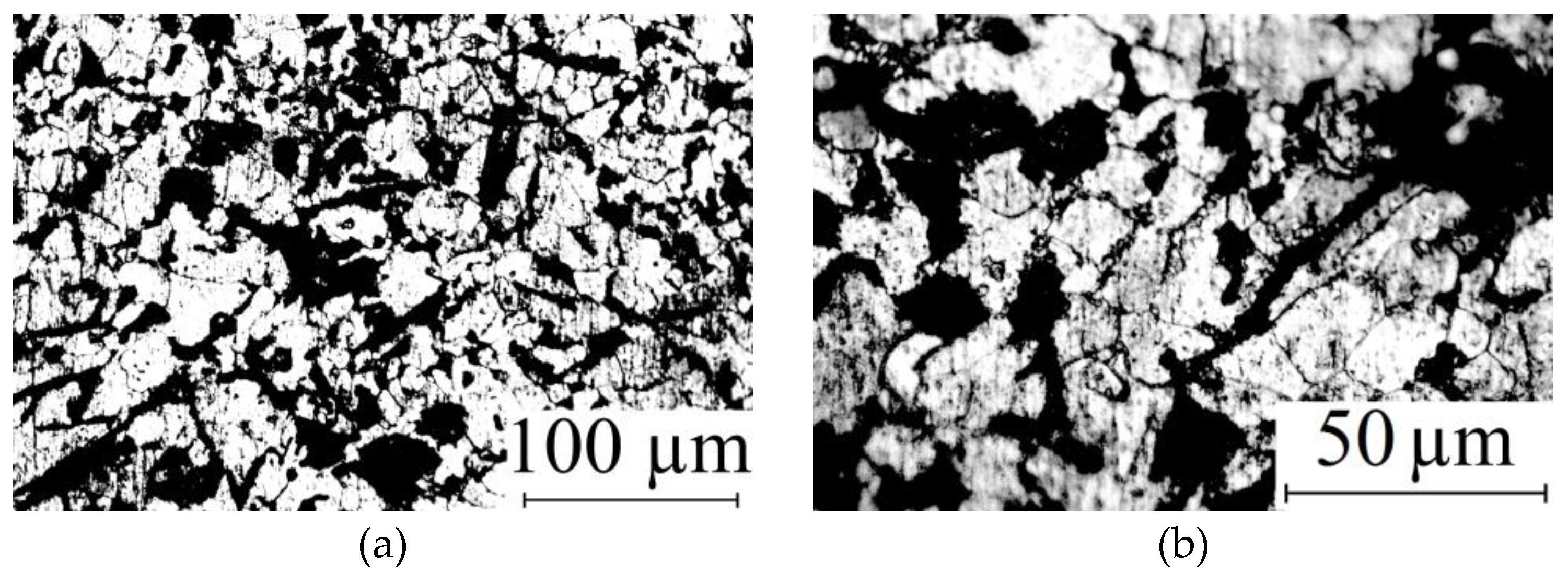
2. Experimental Procedure
3. Theoretical Procedure
- The stress at the interface boundary of the i-th element and its k-th neighbor at the (n − 1)-th time step is calculated as the difference of hydrostatic pressures acting from each element of the considered pair:
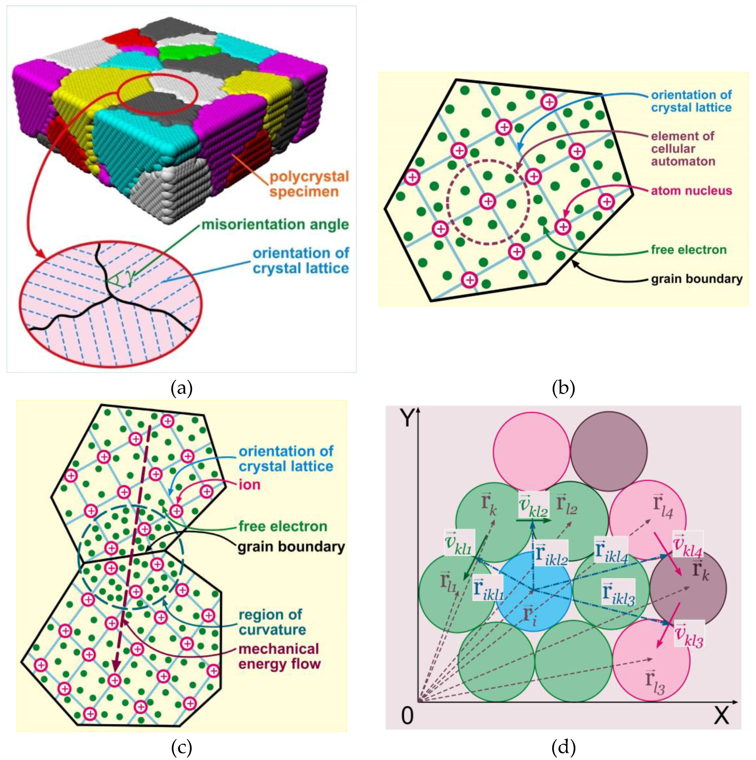
- A relation analogous to the Newtonian viscous flow assuming he proportionality between the force and velocity [3] is used to calculate the average velocity of material points moving through a virtual boundary between fixed elements of space under the action of stress :Here, is the material mobility at the boundary between the i-th element and its k-th neighbor:where , are the elastic moduli of the i-th element and its k-th neighbor, is the number of defects in the active element and is the number of atoms in the active element, c is the effective rate of material response to external mechanical load, is the Boltzmann constant, and is the temperature at the boundary. Here, is the activation energy of the motion of the boundary between the i-th element and its k-th neighbor, which is calculated according to the Read–Shockley approximation, which tacitly assumes that all grain boundaries are of low-angle origin (this is a serious limitation of the model which has yet to be elaborated in the future research) [37]:where is the maximum boundary energy corresponding to the maximum lattice misorientation angle , and is the function that determines the lattice misorientation angle of grains containing the i-th element and its k-th neighbor, 0 ≤ ≤ (Figure 1c). We may conclude from this definition of mobility that the boundary mobility is the reciprocal of the specific (over the volume) momentum of reaction force of the material contained in the neighboring element. Then, we calculate the volume fraction of the substance transferred to the neighboring element () and the mechanical energy change in the i-th element as a result of interaction with its k-th neighbor ():Here, Δτ is the time step, is the element size and is the element volume.
- The total relative volume change () and the mechanical energy change () of the i-th element are found as a result of its interaction with all of nearest neighbors:
4. Results and Discussion
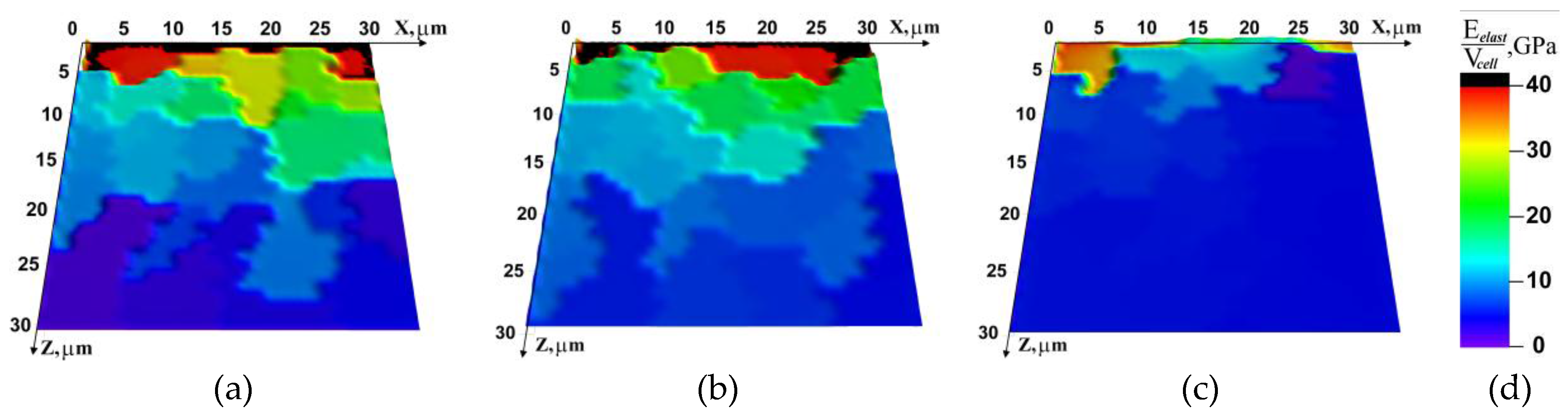
4.1. Simulation of Impact Loading Meso-Dynamics at Different Temperatures
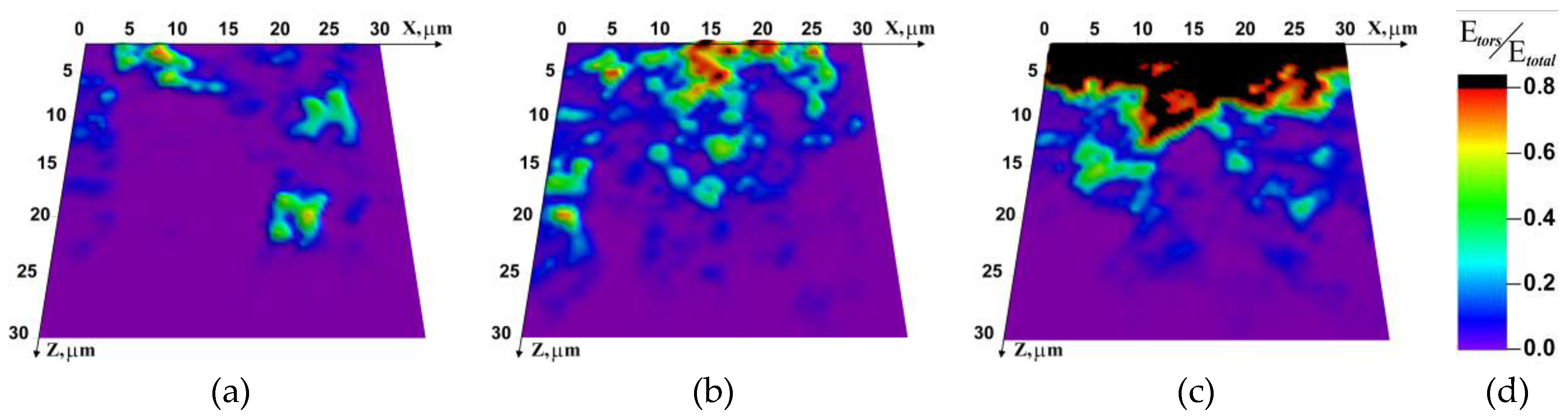
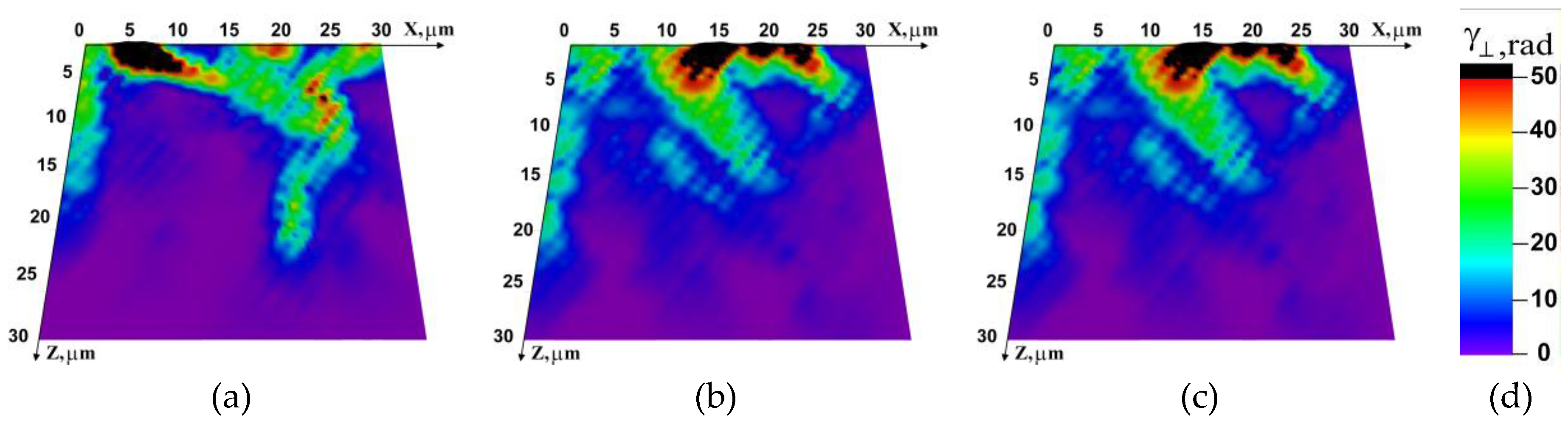
4.2. Fracture Micromechanisms
5. Conclusions
Acknowledgments
Author Contributions
Conflicts of Interest
References
- Panin, V.E.; Egorushkin, V.E. Basic Physical Mesomechanics of Plastic Deformation and Fracture of Solids as Hierarchically Organized Nonlinear Systems. Phys. Mesomech. 2015, 18, 377–390. [Google Scholar] [CrossRef]
- Panin, V.E.; Panin, A.V.; Moiseenko, D.D. Physical mesomechanics of a deformed solid as a multilevel system. II. Chessboard-like mesoeffect of the interface in heterogeneous media in external fields. Phys. Mesomech. 2007, 10, 5–14. [Google Scholar] [CrossRef]
- Moiseenko, D.D.; Panin, V.E.; Elsukova, T.F. Role of local curvature in grain boundary sliding in a deformed polycrystal. Phys. Mesomech. 2013, 16, 335–347. [Google Scholar] [CrossRef]
- Makarov, P.V.; Schmauder, S.; Cherepanov, O.I.; Smolin, I.Y.; Romanova, V.A.; Balokhonov, R.R.; Saraev, D.Y.; Soppa, E.; Kizler, P.; Fischer, G.; et al. Simulation of elastic-plastic deformation and fracture of materials at micro-, meso- and macrolevels. Theor. Appl. Fract. Mech. 2001, 37, 183–244. [Google Scholar] [CrossRef]
- Shilkrot, L.E.; Curtin, W.A.; Miller, R.E. A coupled atomistic/continuum model of defects in solids. J. Mech. Phys. Solids 2002, 50, 2085–2106. [Google Scholar] [CrossRef]
- Olson, G.B. Computational Design of Hierarchically Structured Materials. Science 1997, 277, 1237–1242. [Google Scholar] [CrossRef]
- Mura, R.; Ting, T.C.T. Micromechanics of Defects in Solids (2nd rev. ed.). J. Appl. Mech. 1989, 56, 487. [Google Scholar] [CrossRef]
- Ohashi, T.; Kawamukai, M.; Zbib, H. A multiscale approach for modeling scale-dependent yield stress in polycrystalline metals. Int. J. Plast. 2007, 23, 897–914. [Google Scholar] [CrossRef]
- Kouznetsova, V.; Geers, M.G.D.; Brekelmans, W.A.M. Multi-scale constitutive modelling of heterogeneous materials with a gradient-enhanced computational homogenization scheme. Int. J. Numer. Methods Eng. 2002, 54, 1235–1260. [Google Scholar] [CrossRef]
- Kouznetsova, V.G.; Geers, M.G.D.; Brekelmans, W.A.M. Multi-scale second-order computational homogenization of multi-phase materials: A nested finite element solution strategy. Comput. Methods Appl. Mech. Eng. 2004, 193, 5525–5550. [Google Scholar] [CrossRef]
- Miehe, C. Computational micro-to-macro transitions discretized micro-structures of heterogeneous materials at finite strains based on the minimization of averaged incremental energy. Comput. Methods Appl. Mech. Eng. 2003, 192, 559–591. [Google Scholar] [CrossRef]
- Panin, V.E.; Egorushkin, V.E.; Panin, A.V.; Chernyavskii, A.G. Plastic distortion as a fundamental mechanism in nonlinear mesomechanics of plastic deformation and fracture. Phys. Mesomech. 2016, 19, 255–258. [Google Scholar] [CrossRef]
- McDowell, D.L. A perspective on trends in multiscale plasticity. Int. J. Plast. 2010, 26, 1280–1309. [Google Scholar] [CrossRef]
- Zhu, T.; Li, J.; Samanta, A.; Leach, A.; Gall, K. Temperature and strain-rate dependence of surface dislocation nucleation. Phys. Rev. Lett. 2008, 100. [Google Scholar] [CrossRef] [PubMed]
- Chen, L.Y.; He, M.; Shin, J.; Richter, G.; Gianola, D.S. Measuring surface dislocation nucleation in defect-scarce nanostructures. Nat. Mater. 2015, 14, 707–713. [Google Scholar] [CrossRef] [PubMed]
- Nicola, L.; Bower, A.F.; Kim, K.S.; Needleman, A.; Van der Giessen, E. Surface versus bulk nucleation of dislocations during contact. J. Mech. Phys. Solids 2007, 55, 1120–1144. [Google Scholar] [CrossRef]
- Gale, W.F.; Totemeir, T.C. Smithells Metals Reference Book; Elsevier Butterworth-Heinemann: Oxford, UK, 2004. [Google Scholar]
- Pyshmintsev, I.Y.; Struin, A.O.; Gervasyev, A.M.; Lobanov, M.L.; Rusakov, G.M.; Danilov, S.V.; Arabey, A.B. Effect of bainite crystallographic texture on failure of pipe steel sheets made by controlled thermomechanical treatment. Metallurgist 2016, 60, 405–412. [Google Scholar] [CrossRef]
- Nykyforchyn, H.; Lunarska, E.; Tsyrulnyk, O.T.; Nikiforov, K.; Genarro, M.E.; Gabetta, G. Environmentally assisted “in-bulk” steel degradation of long term service gas trunkline. Eng. Fail. Anal. 2010, 17, 624–632. [Google Scholar] [CrossRef]
- Yasnikov, I.S.; Vinogradov, A.; Estrin, Y. Revisiting the Considère Criterion from the Viewpoint of Dislocation Theory Fundamentals. Scr. Mater. 2014, 76, 37–40. [Google Scholar] [CrossRef]
- Vinogradov, A. Mechanical Properties of ultrafine grained metals: New challenges and perspectives. Adv. Eng. Mater. 2015, 17, 1710–1722. [Google Scholar] [CrossRef]
- Lehto, P.; Remes, H.; Saukkonen, T.; Hänninen, H.; Romanoff, J. Influence of grain size distribution on the Hall-Petch relationship of welded structural steel. Mater. Sci. Eng. A 2014, 592, 28–39. [Google Scholar] [CrossRef]
- Zhuang, Z.; O’Donoghu, P.E. The recent development of analysis methodology for rapid crack propagation and arrest in gas pipelines. Int. J. Fract. 2000, 101, 269–290. [Google Scholar] [CrossRef]
- Han, Y.; Shi, J.; Xu, L.; Cao, W.Q.; Dong, H. Effect of hot rolling temperature on grain size and precipitation hardening in a Ti-microalloyed low-carbon martensitic steel. Mater. Sci. Eng. A 2012, 553, 192–199. [Google Scholar] [CrossRef]
- Farber, V.M.; Pyshmintsev, I.Yu.; Arabei, A.B.; Selivanova, O.V.; Polukhina, O.N. Contributions of structural factors to the strength of K65 steels. Steel Transl. 2012, 42, 687–690. [Google Scholar] [CrossRef]
- Bhattacharjee, D.; Knott, J.F.; Davis, C.L. Charpy-impact-toughness prediction using an “Effective” grain size for thermomechanically controlled rolled microalloyed steels. Metall. Mater. Trans. A 2004, 35, 121–130. [Google Scholar] [CrossRef]
- Smirnov, M.A.; Pyshmintsev, I.Y.; Maltseva, A.N.; Mushina, O.V. Effect of ferrite-bainite structure on the properties of high-strength pipe steel. Metallurgist 2012, 56, 43–51. [Google Scholar] [CrossRef]
- O’Donoghue, P.E.; Kanninen, M.F.; Lueng, C.P.; Demofonti, G.; Venzi, S. The development and validation of a dynamic fracture propagation model for gas transmission pipelines. Int. J. Press. Vessels Pip. 1997, 70, 11–25. [Google Scholar] [CrossRef]
- Pyshmintsev, I.Y.; Boryakova, A.N.; Smirnov, M.A.; Krainov, V.I. Influence of the plastic-deformation temperature on the structure and properties of low-carbon pipe steel. Steel Transl. 2010, 40, 21–26. [Google Scholar] [CrossRef]
- Tsuji, N.; Okuno, S.; Koizumi, Y.; Minamino, Y. Toughness of Ultrafine Grained Ferritic Steels Fabricated by ARB and Annealing Process. Mater. Trans. 2004, 45, 2272–2281. [Google Scholar] [CrossRef]
- Safarov, I.M.; Korznikov, A.V.; Galeyev, R.M.; Sergeev, S.N.; Gladkovsky, S.V.; Pyshmintsev, I.Y. An anomaly of the temperature dependence of the impact strength of low-carbon steel with an ultrafine-grain structure. Dokl. Phys. 2016, 61, 15–18. [Google Scholar] [CrossRef]
- Zhao, R.; Han, J.Q.; Liu, B.B.; Wan, M. Interaction of forming temperature and grain size effect in micro/meso-scale plastic deformation of nickel-base superalloy. Mater. Des. 2016, 94, 195–206. [Google Scholar] [CrossRef]
- Kouznetsova, V.; Brekelmans, W.A.M.; Baaijens, F.P.T. Approach to micro-macro modeling of heterogeneous materials. Comput. Mech. 2001, 27, 37–48. [Google Scholar] [CrossRef]
- Armstrong, R. The influence of polycrystal grain size on several mechanical properties of materials. Metall. Mater. Trans. B 1970, 1, 1169–1176. [Google Scholar] [CrossRef]
- Hwang, B.; Kim, Y.G.; Lee, S.; Kim, Y.M.; Kim, N.J.; Yoo, J.Y. Effective grain size and charpy impact properties of high-toughness X70 pipeline steels. Metall. Mater. Trans. A 2005, 36, 2107–2114. [Google Scholar] [CrossRef]
- Mirzaev, D.A.; Schastlivtsev, V.M.; Yakovleva, I.L.; Tereshchenko, N.A.; Shaburov, D.V. The formation of delamination cracks in impact-toughness tests as a cause of the increase in the impact toughness of steels with bcc structure. Phys. Met. Metallogr. 2015, 116, 1253–1258. [Google Scholar] [CrossRef]
- Priester, L. Grain Boundaries; Springer Series in Materials Science 172; Springer Science+Business Media: Dordrecht, The Netherlands, 2013. [Google Scholar]
- Chernov, V.M.; Kardashev, B.K.; Moroz, K.A. Low-temperature embrittlement and fracture of metals with different crystal lattices—Dislocation mechanisms. Nucl. Mater. Energy 2016, 9, 496–501. [Google Scholar] [CrossRef]
- Benac, D.J.; Cherolis, N.; Wood, D. Managing Cold Temperature and Brittle Fracture Hazards in Pressure Vessels. J. Fail. Anal. Prev. 2016, 16, 55–66. [Google Scholar] [CrossRef]
- Hansen, N. Hall-petch relation and boundary strengthening. Scr. Mater. 2004, 51, 801–806. [Google Scholar] [CrossRef]
- Shin, S.Y.; Hwang, B.; Lee, S.; Kim, N.J.; Ahn, S.S. Correlation of microstructure and charpy impact properties in API X70 and X80 line-pipe steels. Metall. Mater. Trans. A 2007, 458, 281–289. [Google Scholar] [CrossRef]
- Panin, S.; Vinogradov, A.; Moiseenko, D.; Maksimov, P.; Berto, F.; Byakov, A.; Eremin, A.; Narkevich, N. Numerical and Experimental Study of Strain Localization in Notched Specimens of a Ductile Steel on Meso- and Macroscales. Adv. Eng. Mater. 2016, 18, 2095–2106. [Google Scholar] [CrossRef]
- Margolin, B.Z.; Shvetsova, V.A. Brittle fracture criterion: Structural mechanics approach. Strength Mater. 1992, 24, 115–131. [Google Scholar] [CrossRef]
- Goritskii, V.M.; Shneyderov, G.R.; Lushkin, M.A. Nature of anisotropy of impact toughness of structural steels with ferrite-pearlite structure. Phys. Met. Metall. 2013, 114, 877–883. [Google Scholar] [CrossRef]
- Panin, S.V.; Maruschak, P.O.; Vlasov, I.V.; Moiseenko, D.D.; Berto, F.; Vinogradov, A. Effect of temperature-force factors and concentrator shape on impact fracture mechanisms of 17Mn1Si steel. Adv. Mater. Sci. Eng. 2017, 2017, 12. [Google Scholar] [CrossRef]


| T, °C | −60 | −40 | −20 | 0 | 20 |
|---|---|---|---|---|---|
| KCV, J/cm2 | 9.3 ± 2 | 20 ± 3 | 46 ± 9 | 60 ± 10 | 73.3 ± 12 |
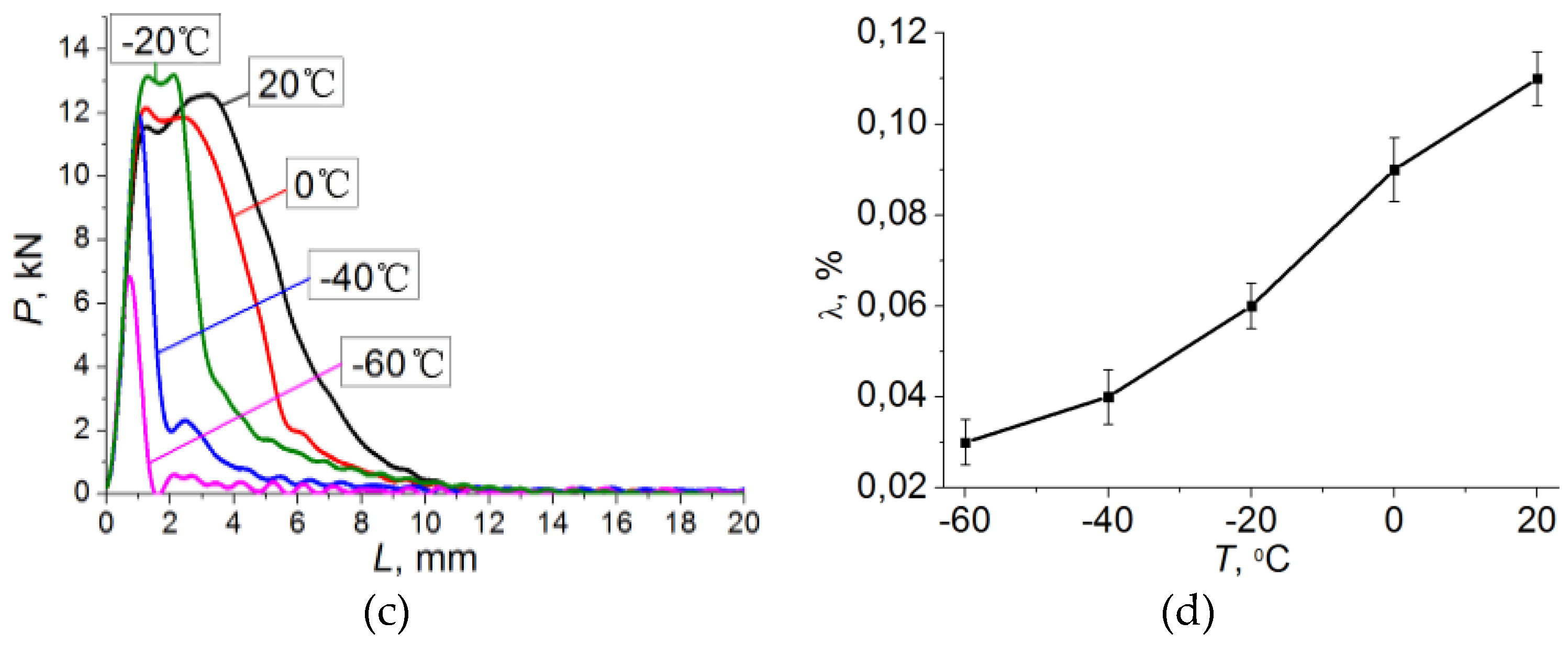
| λ, % | 0.03 ± 0.005 | 0.04 ± 0.006 | 0.06 ± 0.005 | 0.09 ± 0.007 | 0.11 ± 0.006 |
| Temperature, K (°C) | 213.2 (−60) | 233.2 (−40) | 253.2 (−20) | 273.2 (0) | 293.2 (20) |
|---|---|---|---|---|---|
| kdiss | 250 | 500 | 1000 | 2000 | 4000 |
© 2017 by the authors. Licensee MDPI, Basel, Switzerland. This article is an open access article distributed under the terms and conditions of the Creative Commons Attribution (CC BY) license (http://creativecommons.org/licenses/by/4.0/).
Share and Cite
Moiseenko, D.; Maruschak, P.; Panin, S.; Maksimov, P.; Vlasov, I.; Berto, F.; Schmauder, S.; Vinogradov, A. Effect of Structural Heterogeneity of 17Mn1Si Steel on the Temperature Dependence of Impact Deformation and Fracture. Metals 2017, 7, 280. https://doi.org/10.3390/met7070280
Moiseenko D, Maruschak P, Panin S, Maksimov P, Vlasov I, Berto F, Schmauder S, Vinogradov A. Effect of Structural Heterogeneity of 17Mn1Si Steel on the Temperature Dependence of Impact Deformation and Fracture. Metals. 2017; 7(7):280. https://doi.org/10.3390/met7070280
Chicago/Turabian StyleMoiseenko, Dmitry, Pavlo Maruschak, Sergey Panin, Pavel Maksimov, Ilya Vlasov, Filippo Berto, Siegfried Schmauder, and Alexey Vinogradov. 2017. "Effect of Structural Heterogeneity of 17Mn1Si Steel on the Temperature Dependence of Impact Deformation and Fracture" Metals 7, no. 7: 280. https://doi.org/10.3390/met7070280