Inspection of Prebaked Carbon Anodes Using Multi-Spectral Acousto-Ultrasonic Excitation
by
Moez Ben Boubaker
1, 
Donald Picard
2,
Carl Duchesne
1,*,
Jayson Tessier
3,
Houshang Alamdari
4 and
Mario Fafard
2 1
Aluminium Research Centre—REGAL, Département de Génie Chimique, Université Laval, Québec, QC G1V 0A6, Canada
2
Aluminium Research Centre—REGAL, Département de Génie Civil, Université Laval, Québec, QC G1V 0A6, Canada
3
Alcoa Primary Metals Smelting Center of Excellence, Québec, QC G0A 1S0, Canada
4
Aluminium Research Centre—REGAL, Département de Génie des Mines, de la Métallurgie et des Matériaux, Université Laval, Québec, QC G1V 0A6, Canada
*
Author to whom correspondence should be addressed.
Metals 2017, 7(8), 305; https://doi.org/10.3390/met7080305
Submission received: 15 June 2017
/
Revised: 2 August 2017
/
Accepted: 5 August 2017
/
Published: 8 August 2017
(This article belongs to the Special Issue Selected Papers from the International Committee for Study of Bauxite, Alumina & Aluminium 2016)
Abstract
:Reduction cell operation in primary aluminum production is strongly influenced by the properties of baked anodes. Producing consistent anode quality is more challenging nowadays due to the increasing variability of raw materials. Taking timely corrective actions to attenuate the impact of raw material fluctuations on anode quality is also difficult based on the core sampling and characterization scheme currently used by most anode manufacturers, because it is applied on a very small proportion of the anode production (about 1%), and long-time delays are required for lab characterization. The objective of this work is to develop rapid and non-destructive methods for the inspection of baked anodes. Previous work has established that sequential excitation of smaller parts collected from an industrial sized anode using acousto-ultrasonic signals at different frequencies allowed detecting and discriminating anode defects (pores and cracks). This was validated qualitatively using X-ray computed tomography. This work improves the method by using frequency-modulated excitation and building quantitative relationships between the acousto-ultrasonic signals and defects extracted from tomography images using Wavelet Transforms and Partial Least Squares (PLS) regression. The new excitation approach was found to provide similar or better inspection performance compared with sequential excitation, while requiring a shorter cycle time.
1. Introduction
Most modern primary aluminum smelters use the Hall-Héroult (H-H) electrochemical process to reduce alumina powder to metal aluminum. To carry out the reaction, prebaked carbon anodes are utilized in order to distribute the electrical current in the reduction cells, and to supply the carbon required by the reaction. Hence, the anodes are consumed and need to be replaced according to a predefined set cycle. The overall performance of the H-H process is strongly influenced by the quality of the anodes blocks. For instance, a low electrical resistivity is important for maximizing energy efficiency. A high mechanical strength and density, and low reactivity to air and CO2 are desirable for minimizing carbon consumption, and for reducing the environmental footprint and greenhouse gas (GHG) emissions. Any physical defects within the anode blocks, such as pores, cracks or compositional heterogeneities, may adversely affect the anode performance, and consequently, the performance of the reduction cells. Producing high quality anodes consistently is therefore a major concern for the manufacturers who are currently facing degrading quality, and increasing variability and cost of the anode raw materials (petroleum coke and coal tar pitch).
The traditional anode quality control scheme used by the industry and consisting of collecting core samples from the baked anodes and characterizing them in the laboratory is inadequate to address the current needs. Indeed, core samples are gathered from a very small proportion of the anode production (often less than 1%) because of the destructive and time/resource consuming nature of the procedures. Furthermore, the samples themselves represent only 0.1–0.2% of the anode block volume, which has properties known to be anisotropic. Finally, the core sample properties are typically available only after a long time delay, which limits the implementation of feedback corrective adjustments to the anode manufacturing process when deemed necessary. Therefore, alternative rapid and non-destructive techniques are required to assess the quality of individual baked anodes before they are set in the H-H reduction cells.
Recent research efforts focused on developing devices for measuring the electrical resistivity of the individual green [1,2,3] and baked [4,5] anode blocks using different technologies. These sensors allow measurement of a very important anode property related with energy efficiency, but their capacity to detect, locate and diagnose physical defects within the anode blocks has yet to be established. Alternatively, the performance of acousto-ultrasonic (AU) techniques for detection of various defects in carbon anodes has been demonstrated in previous work [6] using sequential acoustic excitation at different frequencies. Sliced anode samples were tested using this approach and their acoustic responses was analyzed using Principal Component Analysis (PCA). The relationship between the attenuation of the acoustic signals and the presence of different defects was validated qualitatively using X-ray images collected from the slices. However, sequential excitation at multiple points on the material is a lengthy process, and shortening the cycle time of the acoustic inspection scheme is highly desirable for industrial implementation.
The aim of this work was to demonstrate that exciting the anode materials using a single frequency modulated acoustic wave (multi-frequency signal) can lead to similar or better results compared to sequential excitation, while significantly reducing cycle time. For instance, the sequential excitation scheme used in previous work to obtain good inspection results consisted of testing the materials at seven excitation frequencies in the 100–250 kHz range for each measurement point [6]. A single frequency modulated wave in the same range would reduce cycle time by 7 to 1 for the same number of data points. A side objective of this work was to validate the proposed approach more quantitatively, by building empirical regression models between the acoustic response of the materials and the corresponding Computed Tomography-scan images. These images were used for the sole purpose of confirming the inspection results, as they would not be available in an industrial implementation.
Under frequency-modulated excitation, the material response signal is more complex as it also contains multiple frequencies. To quantify the acoustic attenuation at different frequencies, the signal needs to be first decomposed. One approach consists of using the Fast-Fourier transform (FFT) [7,8,9,10]. However, this method only performs frequency domain decomposition and does not capture variations in the signal frequency content through time, which may limit performance in defect detection and identification. An alternative approach is to perform time-frequency decomposition of the signals using Wavelet Transforms (WT) [11,12,13,14], which were shown to be a powerful tool in all areas dealing with transient signals [15,16,17]. Qi et al. [18,19] showed the effectiveness of the Discrete Wavelet Transform (DWT) for processing acousto-ultrasonic signals collected from composite materials. A similar approach was used in this work.
To quantify defects in tomographic images, texture analysis techniques were used, since the defects introduce local variations in grey level intensity in the images according to some relatively well-defined patterns (e.g., round spots for pores and streak lines for cracks). Again here, one could extract textural features from tomographic images using the two-dimensional Fast Fourier Transform (2D-FFT) [20]. The frequency decomposition of the images could be used to determine the severity of the defects. However, variations in frequency content within the images (i.e., spatial information) cannot be extracted using this approach. On the other hand, the 2D Discrete Wavelet Transform (2D-DWT) is effective for extracting both frequency and spatial information [21]. Wavelet texture analysis has proved a useful tool in several areas dealing with noise and low variation in images.
After applying the WT to both sets of data (acoustic signals and images), wavelet features were extracted and analyzed using PCA in order to explore the clustering pattern of the various anodes slices. A regression model was then built between both data sets. The results showed that the attenuated acoustic response of the materials obtained after frequency-modulated excitation was sensitive to the presence of cracks within anode samples, and to the density of pores distributed throughout the anode samples (slices). The performance of this approach was found to be similar to that obtained using sequential excitation [6], but with a significant reduction in cycle time.
2. Materials and Experimental Data Acquisition
2.1. Baked Anode Samples and X-ray Images
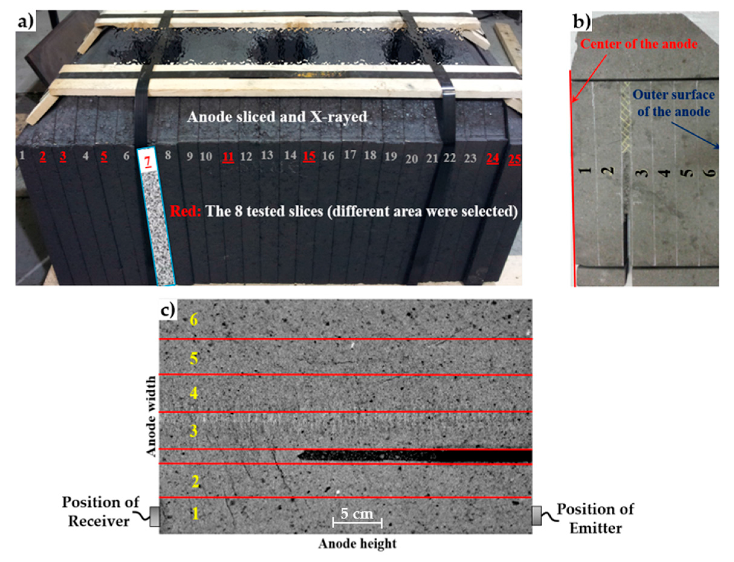
A full-size industrial baked carbon anode was scanned using a Siemens Somatom Sensation 64 tomograph (512 × 512 pixels) (Siemens Healthcare GmbH, Erlangen, Germany). The scanning area of the X-ray apparatus was limited to objects of less than a 40 × 40 mm2 cross-section. Since the anode was too large to fit in the scanning area in one piece, it was cut in several slices, as shown in Figure 1. The cutting was performed with care to avoid altering any anode defects. Furthermore, for a single CT image reconstruction, a higher image resolution is obtained when the samples are smaller in size (down to a cross-section of 50 × 50 mm2 where the resolution limit of the tomograph used is reached), which increases the contrast between defects and the background [22]. The anode was first cut into 26 slices (Figure 1a), and then each of them were cut further in halves along their heights (Figure 1b). The top and bottom of each half slice was also cut to obtain samples of uniform geometry before collecting the acoustic response of the material. Note that the following eight slices were selected for further AU analysis: 2, 3, 5, 7, 11, 15, 24 and 25 (indicated using red numbers in Figure 1a). These slices spanned a range of internal structures, and were selected from areas which were expected to contain different types of defects, such as pores and cracks (see [6] for more details).
The CT-scan measured the attenuation coefficients of the material for a set of 512 × 512 3D voxel (volumetric pixel) per scan, which corresponded to the tomograph resolution. Given the slice dimensions, the voxels had a resolution of 0.7 × 0.6 × 0.7 mm3. The X-ray attenuation coefficients of the voxels (also called Computed Tomography or CT numbers) were converted to grayscale images showing spatial variations correlated with the materials density [22,23]. Cracks and pores appear as groups of dark pixels surrounded by lighter background (carbon material). The high-density impurities appear as bright pixels inside a darker background. Figure 1c shows an example X-ray image for one slice.
2.2. Acousto-Ultrasonic (AU) Signal Acquisition
The acousto-ultrasonic inspection system used in this work was described in detail in [6]. It consisted of a multi-channel acousto-ultrasonic apparatus using two acoustic sensors (an emitter and a receiver), a pre-amplifier, and a software for controlling the excitation and recording the emission signals. After testing several sets of sensors, it was found that using transducers having a resonant frequency at 55 kHz provided the best results for the tested materials. The sensors were mounted on both ends of the anode slices (one on top and the other on the bottom surface) using mechanical clamps. Coupling gel was applied on the anode surfaces before the sensors were put into contact with the materials. This was made to ensure good contact between the sensors and the anode samples, which typically have rough surfaces. The sensors were placed vis-à-vis each other, and moved together along the anode width to measure the AU response of the materials included in the six so-called corridors (identified by white chalk in Figure 1b, and by red lines in Figure 1c). The material structure clearly changed from the center of the anodes to the external surface (corridor 1 and 6 in Figure 1c, respectively), as shown by variations in material density (i.e., gray level) and the presence of pores and cracks. As mentioned in the previous section, such variations in the material structure are also expected along the length of the anode (i.e., various slices).
The excitation signal was specified as a modulated frequency signal between 100 and 300 kHz as shown in Figure 2. This range was selected based on previous work [6]. The AU measurements were made using a pre-amplification gain of 40 dB, and sampling rate of 1000 kHz. The selected sampling rate is sufficiently fast to avoid aliasing at frequencies lower than 300 kHz. This procedure was repeated for all six corridors (Figure 1b,c) in each of the selected anode slices. Note that the type of transducer and measurement settings may need to be slightly adjusted if the system is to be used for inspecting anodes from different manufacturers.
3. Extraction of Features from Acoustic Signals and X-ray Images
3.1. Acousto-Ultrasonic Signals
The majority of the acousto-ultrasonic signals propagating through the porous anode materials are in the frequency range of 100–300 kHz. Dividing this range into a set of consecutive frequency bands may help relate different time-frequency features of AU signals to various anodes defects. The wavelet transforms were used to decompose the signals and extract meaningful time-frequency domain features from them.
The decomposition of a continuous 1D signal x(t) using a specific scaled or dilated mother wavelet Ψ (t,a,b) is obtained by the convolution of both the signal and the wavelet function as follows [21]:
In the above Equation, Ψ (t) is the mother wavelet function, which corresponds to a wave of finite length and having a particular shape. Several types of mother wavelets exist (e.g., Haar, Daubechies, Coiflet, Symlet, Mexican Hat, etc.), and they mainly differ by their shape (frequency content). The type of mother wavelet is typically selected to match the shape of the signal x(t) the best possible. The Daubechies wavelet (Db5) was selected in this work. This choice came after selecting the best results from trying several different mother wavelets. Parameters a and b are called the scaling and the translation parameters, respectively. The former stretches the mother wavelet and changes its frequency content, while the latter performs a translation of the wavelet over time. The result of the convolution is a scalar quantity da,b, called the wavelet detail coefficient. It represents how well the signal x(t) matches the dilated mother wavelet at scale a and time point b. Changing the scaling coefficient a from a small to a large value progressively dilates the wavelet and therefore allows extracting information about signal x(t) from high to low frequency. Translating the wavelet using parameter b from the beginning to the end of the x(t) signal allows information to be captured at different time points. Hence, changing a and b in a nested fashion performs a spatial-frequency decomposition of signal x(t), and how well the signal matches the wavelet at scale a and time point b is quantified by the detail coefficient da,b. Note that the acoustic signals analyzed in this work are discrete (i.e., sampled at a given frequency). A discrete version of Equation (1) exists for discrete signals as well. This leads to the so-called Discrete Wavelet Transform (DWT). Values taken by parameters a and b are constrained for computing efficiency and to avoid signal aliasing. For more details on the DWT, the reader is referred to [21].
After performing the wavelet decomposition of the discrete signal x(i), a set of vectors of detail coefficients da(i) were obtained, one for each scale a. Each vector contained the detail coefficient at a given scale but for all time points. In other words, the original signal x(i) was decomposed into a set of detail signals da(i), each containing information in a certain frequency band. Three time domain features were then calculated from each time series da(i), i = 1, 2, …, N, N being the number of samples in the time series. These features are the maximum (MAX), the root mean square (RMS) and the time of flight, or arrival time (AT). These features are calculated as follows:
The acoustic response of the materials x(i) was decomposed up to level 4 (four different discrete values of a) and the MAX and RMS features were calculated from each of them as well as the arrival time. Figure 3 provides an example of a raw acoustic signal decomposed into 4 frequency bands (details 1–4), and also shows the residual signal after four decomposition levels (called approximation).
The data were then collected in a (48 × 15) dimensional matrix X. The 15 columns correspond to the three features computed from the four wavelet detail signals, as well as the approximation for all of the 48 samples (six corridors × eight anode slices). Signal and image processing were performed using Matlab version R2014a (MathWorks, Natick, MA, USA).
3.2. X-ray Image Texture Analysis
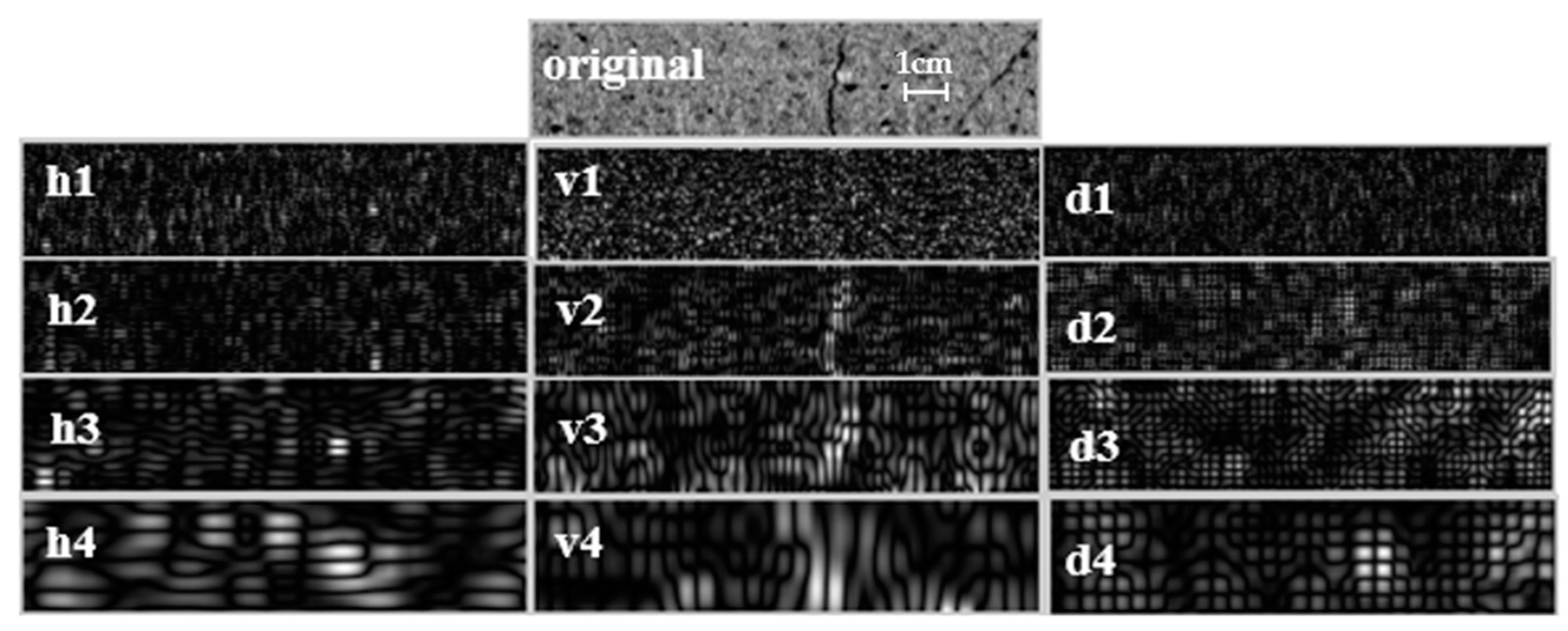
The texture of X-ray images was analyzed using a very similar approach as for the acoustic signals. The tomography data were first converted to grayscale images. The Discrete Wavelet Transform was then applied to them. The main difference in the application of wavelets to images and acoustic signals is that images were 2D signals. An image is a matrix of data I(nX,nY) where nX and nY are the number of pixels in the horizontal and vertical directions in the images and the elements of that matrix correspond to the X-ray attenuation coefficients converted to grayscale values. The convolution between a mother wavelet and the image signals (i.e., discretized version of Equation (1)) is performed along each row and each column of the image (horizontally and vertically) as well as diagonally using a filter bank [21]. Wavelet detail coefficients were obtained for each pixel of the images at each scale and for each of the three directions. These were collected into matrices Djk where j corresponds to the scale, k to each direction (h, v, d), and each element of these matrices match the detail coefficient at a certain pixel location (nX, nY). These matrices can also be displayed as images for visual interpretation, and are typically called wavelet detail sub-images (Djh, Djv, Djd). At the first scale, high frequency information is captured from the images in all three directions, and these are associated with small objects or patterns in the image. As the scale increases, lower frequency information introduced by larger objects or patterns is extracted. The 5th order Daubechies wavelet (Db5) wavelet was selected for extracting textural information from the X-ray images.
Several scalar textural descriptors or textural features can be calculated from the wavelet detail sub-images, the most popular being the energy, variance, entropy, and the mean [24,25]. Our results showed that the energy is sufficient to extract information related with anode defects (pores and cracks) within the X-ray images. The energy is calculated as follows from the wavelet detail sub-images at each scale and for the three directions:
where Djk is the detail coefficient for pixel located at the (nX, nY) position within an image in the kth direction (k = h, v, d) and at the jth scale. The total number of pixels within the images (nX × nY) was used to normalize the energy values. The X-ray images were decomposed up to scale 4. This yielded 12 energy values per anode corridor (four scales × three directions). These values were collected for the 48 corridors and stored in matrix Y of dimensions (48 × 12).
The application of wavelet decomposition to one such X-ray image is shown in Figure 4. It displays the original image as well as the detail sub-images for each of the four scales and directions. The sub-images are identified by the direction first (h, v, d) and then by the scale number (1,2,3,4). For instance, sub-images v3 display the information extracted from the image by the wavelet in the vertical direction at scale 3. The vertical and diagonal sub-images at scales 2–4 clearly capture the profile line of the vertical and diagonal cracks in the image. This information was regressed against the acoustic signals in order to link the acoustic attenuation to anode defects quantitatively.
4. Multivariate Statistical Methods for Analysis of the Acousto-Ultrasonic Signal and Image Features
Multivariate statistical methods were used to analyze the large data matrices obtained in this study. First, PCA was used to cluster the X-ray images based on their texture (Y data). Then, Partial Least Squares (PLS) regression was utilized to build relationships between the acoustic attenuation data (X) and then image textural features (Y). These methods are briefly described below.
4.1. Principal Component Analysis
Data clustering in the latent variable space using methods such as PCA is widely used for the analysis of large datasets containing noisy and highly collinear data. PCA summarizes the variations contained in a large set of J variables X = [x1, x2, …, xJ] by a much smaller number of orthogonal latent variables (or scores) T = [t1, t2, …, tA] (A << J) together capturing the dominant sources of variations in the data. The scores are obtained by an eigenvector-eigenvalue bilinear decomposition of the X matrix and is mathematically expressed as follows [26,27]:
where the orthogonal vectors ta are the latent variables (called scores) providing the coordinates of each sample in the low dimensional subspace (plane or hyperplane) after projection. The subspace itself is defined by the A orthonormal loading vectors pa, which are linear combinations of the original variables (i.e., ta = X pa). The projection residuals are collected in the residual matrix E. The loading vectors are calculated in such a way that t1 explains the greatest amount of variance in X, t2 the second greatest amount of variance not explained by the first component, and so on. Plots of the score values are used to visualize the clustering pattern of the data while the loadings allow interpretation of the patterns by the changes in the variables. The reader is referred to [27] for more details on PCA.
4.2. Partial Least Squares Regression
The PLS regression method was used here to correlate the acousto-ultrasonic features of the anode corridors gathered in the X matrix with corresponding image textural features collected in Y. Similar as for PCA, this regression method has an advantage of overcoming the strong correlation between features in both data blocks. Each PLS latent variable is calculated in such a way as to maximize the covariance in both data matrices and the following model structure is obtained [28,29]:
where the latent variable space of both X and Y corresponds to the scores T (orthogonal PLS components) which relate X to Y. The sub-spaces of X and Y are modeled by the loading matrices P and C, respectively, while the corresponding residuals are stored in E and F. Finally, the so-called weight vectors W* contain the linear combinations that express T in terms of X and predictions of Y to be made.
The PLS method also performs clustering of samples vector in the latent variable subspace according to the Y data. The clustering patterns can be visualized using scatter plots of the scores (t’s). The differences between the clusters can be interpreted using the loading weight vectors (w*’s). The reader is referred to Wold et al. [29] for more details about these methods. The ProMV software version 15.08 (ProSensus, Ancaster, ON, Canada) was used to build PCA and PLS models.
5. Results and Discussion
The X-ray image textural features (Y data) were analyzed first using PCA in order to associate them with anode defects (voids such as pores and cracks). A PLS regression model was then built using both the acoustic and image textural features in order to correlate them. This provided a quantitative validation of the impact of anode defects on the acousto-ultrasonic features.
5.1. Texture Analysis of X-ray Images
Using the cross-validation procedure [30], two PCA components (or latent variables) were found to be significant, and together explained most of the variations in the image textural features. The cumulative sum of squares explained (R2) and predicted (Q2) by the first two PCA components are provided in Table 1. The first two components were found to be sufficient to discriminate the corridors based on their textural features since they explained over 83% of variance in the textural features stored in Y (Q2 = 83.21% in Table 1).
The main variability directions in the image dataset captured by the two PCA components are presented in the t1–t2 score plot shown in Figure 5. Each marker in this plot represents a summary of the textural features of one particular corridor. These are identified by the slice number followed by the corridor number. Corridors having similar textural features cluster close to each other, while those having different features cluster in different locations in the latent variable space. It was observed that the corridors located in the same position within the slices cluster together (see markers of the same color in Figure 5). Furthermore, each group was discriminated from the others along both PCA components, except those of slice number 25. This slice was located close to the corner of the anode block, and contained larger pores and cracks, which made them similar to either corridors #1–2, which typically contained several cracks, or to corridors #6 that contained many pores. This explained why the corridors of slice #25 clustered close to corridors #1–2 or #6.
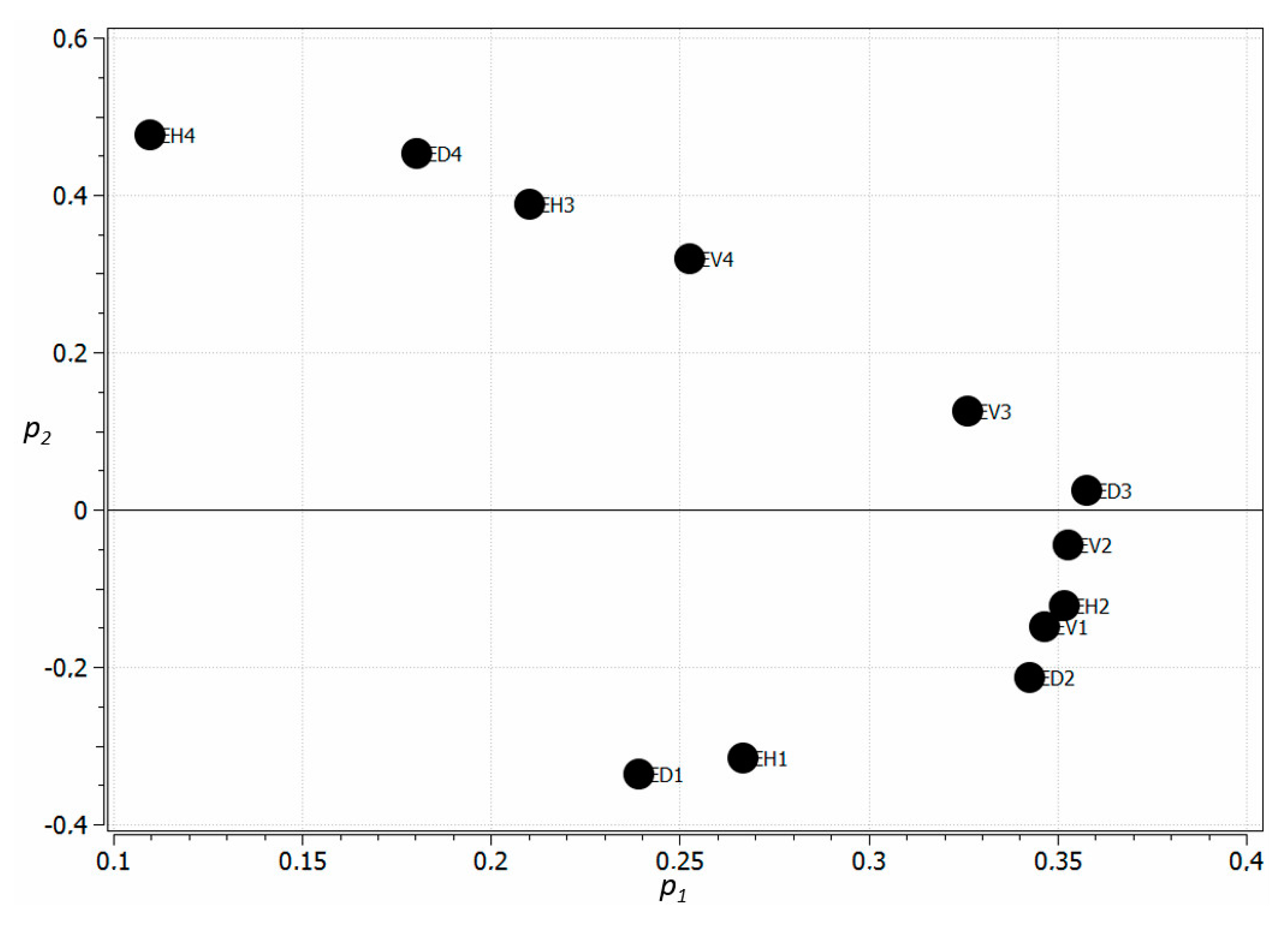
The clustering pattern in the score space can be interpreted based on changes in the textural features by examining the p1–p2 loading plot shown in Figure 6. Each point in the loading plot corresponds to one textural feature calculated from the image of each corridor. They are labeled according to the feature name followed by the wavelet decomposition level. The loading values define the weight of each textural features in each component. The higher the absolute value of the loadings the more important the features are in a given component. The signs of the loadings indicates the sign of their correlation. Features having loading values of the same sign are positively correlated, and those having opposite signs are negatively correlated. The loading plot reveals that the first component is driven by the features in most wavelet decomposition levels, and all of them have loading values of the same sign (i.e., they vary all together in the same direction). This component seems to explain variations in density and/or the total volume of voids (i.e., defect severity) across the X-ray images. A denser region is characterized by higher CT numbers, and hence by higher grey levels in the image. This typically leads to higher energy values as calculated from the wavelet texture analysis. Since corridors 3–4 (and 5 to some extent) were known to be denser, it was expected that these corridors would fall in the positive t1 region (see Figure 5) because the energies at all scales and directions would be higher. On the contrary, corridors 1–2 and 6 typically contained more defects (cracks and pores), and therefore are were less dense, with lower CT numbers, grey level intensities and energies. Thus, it was expected that these would fall in the negative t1 region of the score plot. This clustering pattern along t1 is indeed observed in Figure 5.
The second component, however, was driven by a contrast between the energies at scales 1–2 vs. 3–4, since these two groups have loading values of opposite signs. This component seemed to capture textural variation that corresponded to defects size. Corridors containing larger defects (e.g., cracks) should be characterized by higher energies at lower frequencies (scales 3–4) and lower energy at higher frequencies (scales 1–2) since the lower frequency bands are associated with larger objects or patterns. Since corridors 1–2 typically contained more cracks, they fell in the positive t2 region (higher energies at scales 3–4 and lower at scales 1–2). The situation was the opposite with corridor 6 typically containing pores (clusters in negative t2 region). Hence, the second PCA component seemed to discriminate the types of defects in the anode samples (i.e., pores vs. cracks).
To conclude this section, the textural features extracted from the X-ray images appeared to capture relevant information about the type of the defects present in the anode slices and their severity. Thus, they can be used to perform supervised clustering of the AU signals collected from the corridors, and allow for a quantitative assessment of the sensitivity of AU signal features to anode defects.
5.2. Regression of X-ray Image Textural Features on Acousto-Ultrasonic Features
Five PLS components were found to be statistically significant by a standard cross-validation procedure [30], and together explained about 40% of the variance of the image features (Y data). The goal here was to use the Y data to perform a kind of supervised clustering of the AU signals based on defects found in the X-ray images, and not to predict the image features (i.e., energies) with high accuracy. The first two PLS components were found to be sufficient to discriminate the samples based on their acousto-ultrasonic features, and therefore, only these components will be discussed in this section.
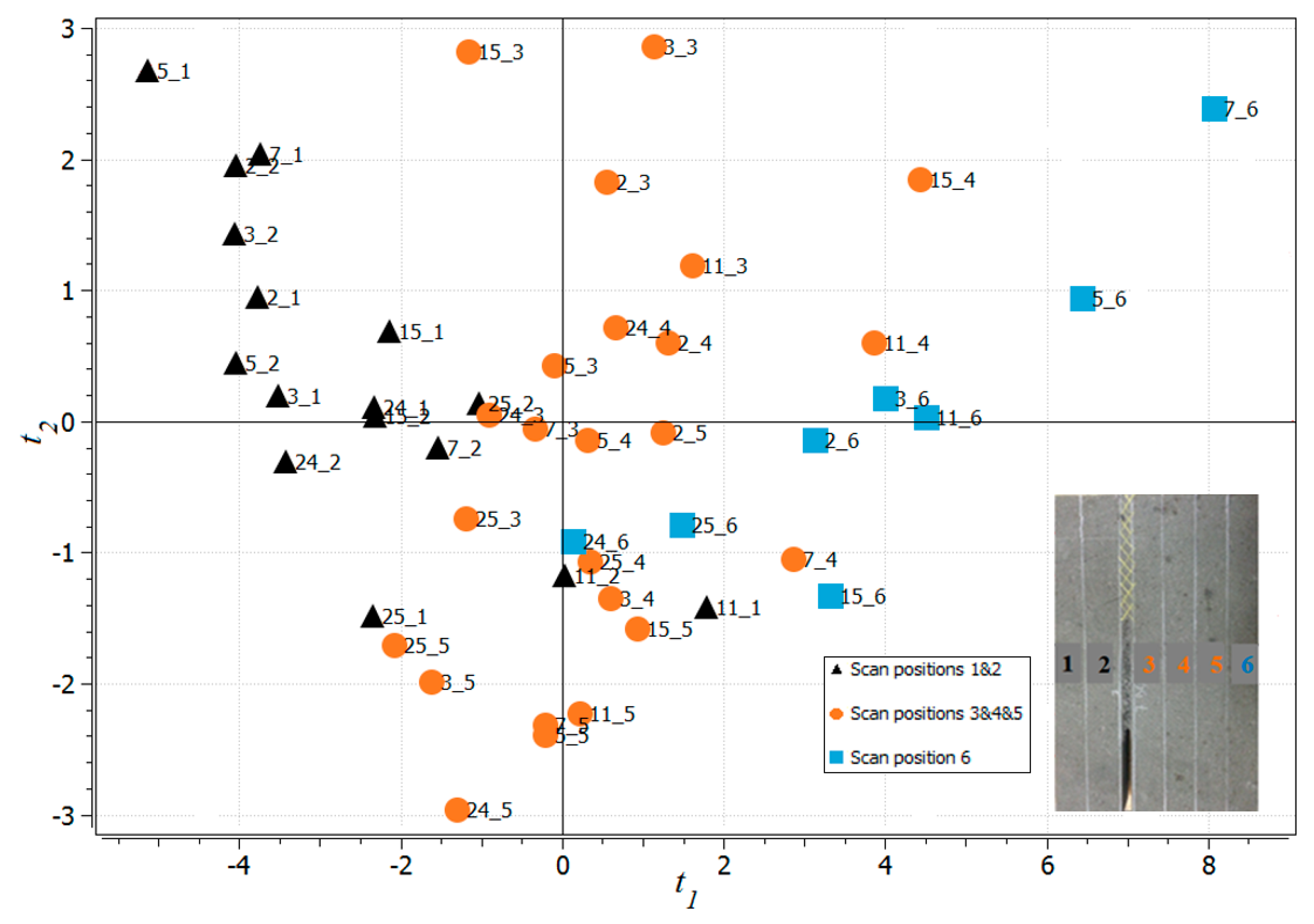
The latent variable score space for the first two components of the PLS model is displayed in Figure 7. Each marker in the plot corresponds to the acousto-ultrasonic response of one corridor, which are identified as described in the previous section. The clustering pattern in the t1–t2 score space reveals that corridors 1–2, 3–5 and 6 of any slice cluster in three groups (black, orange and blue markers, respectively). At this point, it is important to note that corridor #1 was located at the center of the anode, and corridor #6 at the outer surface.
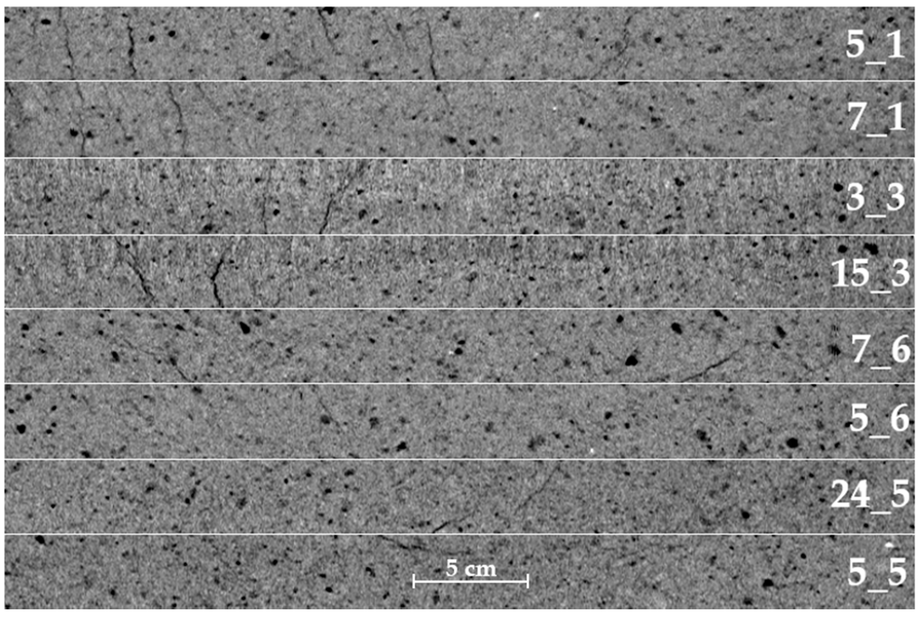
The first component (t1) in Figure 7 seemed to capture the types of defects in the materials, since the corridors where most of the cracks were found (1–2) were located in the negative t1 region. Those characterized by a high concentration of pores (corridor 6) are located in the positive t1 region, and corridors 3–5 containing a mixture of both fall in between the two. The w1*-c1–w2*-c2 loadings bi-plot presented in Figure 8 confirms this interpretation. The signs of X-loadings and Y-loadings (w*’s and c’s or black and red markers in Figure 8) indicate the sign of the correlation between pairs of features whereas their absolute values is proportional to their importance in a given component. Note that comparing the black or the red loading values allows interpretation of the correlation between the acoustic or the image textural features, whereas comparing the black against the red loadings provides information about the cross-correlation between the acoustic and the textural features, and the relationship between both the X and Y datasets. Clearly, the first PLS component captured a similar contrast in the energies at scales 3–4 vs. 1–2 as the second PCA component discussed in the previous section. The variations in the acoustic features (black markers in Figure 8) were also consistent with those in the X-ray image textural features (red markers in Figure 8). When the materials mainly contain cracks, especially when oriented perpendicular to the wave propagation direction, arrival times should be longer, the signals more attenuated (lower MAX and RMS features), and the energies in lower frequency range (scales 3–4) should be higher compared to scales 1–2. Hence, those corridors containing more cracks should fall into the negative t1 region, and those having a higher concentration of pores (and less cracks) should fall in the positive region. This was consistent with the clustering pattern shown in Figure 7. The X-ray images of selected corridors were also shown in Figure 9. Slices 5_1 and 7_1 both had similar t2 values but extremely different t1 scores compared to corridors 5_6 and 7_6. Their X-ray images clearly showed that the former two corridors contained several transversal cracks and some pores, whereas the latter two mostly contains pores, which were also larger.
The second component did not segregate the corridors as much as t1 did, as most of them spanned the t2 range. Since it was orthogonal to the first component, the second component captured a different source of covariation between the acoustic and textural features. The loading plot (Figure 8) shows that all features had the same sign in the t2 component (all positive), although the energies in scales 1–2 and most of the MAX and RMS features (except RMSD4) contributed less in this component. The same sign for these loadings means that they all varied together in the same direction. This was consistent with the first component of the PCA model presented in the previous section, which was associated with variations in material density and/or total volume of voids. Indeed, corridors containing more and larger voids (cracks and/or pores) would lead to longer arrival times, and more energy at scales 3–4 (lower frequencies). Hence, they would project in the positive t2 range compared with corridors containing fewer and smaller voids, which would fall in the negative t2 area. The X-ray images for corridors 3_3 and 15_3 had similar t1 values, but very different t2 scores compared with corridors 5_5 and 24_5. The images in Figure 9 clearly showed that the former two projecting in the high t2 region contain more and larger voids (or defects), compared with the latter two falling in the lower t2 region.
6. Conclusions
Baked carbon anodes are used in the Hall-Héroult aluminum reduction process to distribute the electrical current throughout the cells, and to provide the source of carbon required by the electrolytic reaction. However, poor quality anodes containing structural defects such as cracks, and a high concentration of pores, can deteriorate the reduction cell performance by reducing energy efficiency and increasing carbon consumption. The current quality control scheme based on collecting core samples from a small proportion of the anode production and characterizing them in the laboratory is not adequate for detecting pores and cracks in a rapid and non-destructive fashion. Research efforts are currently being focused on developing new sensors for inspecting individual anode blocks non-intrusively, at a speed compatible with industrial requirements.
Past work have demonstrated the potential of acousto-ultrasonic techniques (AU) to detect pores and cracks in anode samples by using sequential excitation at different frequencies [6]. However, this approach require long cycle times to collect all measurements. The present work aims at reducing cycle times by 7 to 1 using a single frequency-modulated excitation, and showing that such an approach leads to similar inspection results as those obtained with sequential excitation. A quantitative validation of the inspection results is also proposed using X-ray images collected from each sample used in this study.
A full size baked carbon anode was cut into 26 slices of equal thickness. A total of eight slices distributed along the anode length and showing different internal structures were selected for this work. After collecting X-ray images of the samples using a CT-Scan, they were excited by a frequency-modulated wave at 6 different points along the slice width. The AU signal received after the wave propagated through the material at each location (so-called corridors) was recorded. The Discrete Wavelet Transform (DTW) was used to decompose the AU signals into different frequency bands, and to perform texture analysis of the X-ray images. A number of scalar features were subsequently calculated from the wavelet sub-signals and images. Multivariate latent variable methods, such as PCA and PLS regression, were then used to cluster the corridors in each slice according to their internal structure. A regression model was also built between the AU signals and the X-ray images in order to relate variations in the acoustic signals with the presence of defects in the material.
The results showed that the textural features extracted from the X-ray images efficiently detected the voids in the anode samples, and allowed the discrimination of pores from cracks, and captured the severity of those defects. The PLS regression model built between the X-ray image textural and the AU signal features for each corridor clearly showed that variations in the acoustic response of the samples also allowed the detection and discrimination of both types of defects, and assessment of their severity. Furthermore, the inspection results obtained with frequency-modulated excitation led to the same conclusions as those obtained with sequential excitation [6], with a significantly shorter cycle time.
The proposed non-destructive acousto-ultrasonic inspection approach appeared to be very promising for a real-time quality control of industrial scale pre-baked carbon anodes. Future work will investigate the application of the inspection scheme to full size anodes collected from an industrial manufacturing plant. A threshold will then need to be established for AU signals, and will serve as a statistical control limit to determine whether an anode poses a higher risk of deteriorating the reduction cell performance.
Acknowledgments
The authors would like to acknowledge the financial support of the Natural Sciences and Engineering Research Council of Canada (NSERC), Fonds de Recherche du Québec—Nature et Technologies (FRQNT), Alcoa and the Aluminum Research Centre—REGAL. The assistance provided by REGAL personnel, Hugues Ferland and Guillaume Gauvin from Université Laval, in preparing the experimental set up is also greatly acknowledged.
Author Contributions
Moez Ben Boubaker, Donald Picard, Jayson Tessier and Carl Duchesne conceived and designed the experiments; Moez Ben Boubaker and Donald Picard performed the experiments; Moez Ben Boubaker and Carl Duchesne analyzed the data with the support of Mario Fafard and Houshang Alamdari in the results interpretation; Jayson Tessier supplied the materials; Moez Ben Boubaker, Donald Picard and Carl Duchesne wrote the paper; Carl Duchesne, Houshang Alamdari and Mario Fafard revised the paper.
Conflicts of Interest
The authors declare no conflict of interest.
References
- Kocaefe, Y.; Kocaefe, D.; Bhattacharyay, D. Quality Control via Electrical Resistivity Measurement of Industrial Anodes. In Light Metals; John Wiley & Sons: Hoboken, NJ, USA, 2015; pp. 1097–1102. [Google Scholar]
- Andoh, M.A.; Kocaefe, Y.; Kocaefe, D.; Bhattacharyay, D.; Marceau, D.; Morais, B. Mesurement of the Electric Current Distribution in An Anode. In Light Metals; John Wiley & Sons: Hoboken, NJ, USA, 2016; pp. 889–894. [Google Scholar]
- Ziegler, D.P.; Secasan, J. Methods for Determining Green Electrode Electrical Resistivity and Methods for Making Electrodes. U.S. Patent 9,416,458, 16 August 2016. [Google Scholar]
- Chollier-Brym, M.J.; Laroche, D.; Alexandre, A.; Landry, M.; Simard, C.; Simard, L.; Ringuette, D. New Method for Representative Measurement of Anode Electrical Resistance. In Light Metals; John Wiley & Sons: Hoboken, NJ, USA, 2012; pp. 1299–1302. [Google Scholar]
- Léonard, G.; Guérard, S.; Laroche, D.; Arnaud, J.C.; Gourmaud, S.; Gagnon, M.; Marie-Chollier, M.J.; Perron, Y. Anode Electrical Resistance Measurements: Learning and Industrial On-line Measurement Equipment Development. In Light Metals; John Wiley & Sons: Hoboken, NJ, USA, 2014; pp. 1269–1274. [Google Scholar]
- Ben Boubaker, M.; Picard, D.; Duchesne, C.; Tessier, J.; Alamdari, H.; Fafard, M. The Potential of Acousto-Ultrasonic Techniques for Inspection of Baked Carbon Anodes. Metals 2016, 6, 151. [Google Scholar] [CrossRef]
- Suzuki, M.; Nazanishi, H.; Iwamoto, M. Relationship between acoustic emission characteristics and structural factors of composite materials. In Proceedings of the Third Japan-U.S. Conference on Composite Materials, Tokyo, Japan, 23–25 June 1986; pp. 631–638. [Google Scholar]
- Ni, Q.-Q.; Jinen, E. Acoustic emission and fracture of carbon fiber reinforced thermosoftening plastic (CFRTP) materials under monotonous tensile loading. Eng. Fract. Mech. 1993, 45, 611–625. [Google Scholar]
- Ni, Q.-Q.; Jinen, E. Fracture behavior and acoustic emission of SFC. J. Soc. Mater. Sci. 1993, 42, 561–567. [Google Scholar] [CrossRef]
- Ni, Q.-Q.; Jinen, E. Acoustic emission technique in the single-filament-composite test. In Proceedings of the First International Conference on Composite Engineering (ICCE/1), New Orleans, LA, USA, 28–31 August 1994; pp. 883–884. [Google Scholar]
- Serrano, E.P.; Fabio, M.A. Application of the wavelet transform to acoustic emission signal processing. IEEE Trans. Signal Process. 1996, 44, 1270–1275. [Google Scholar] [CrossRef]
- Suzuki, H.; Kinjo, T.; Hayashi, Y.; Takemoto, M.; Ono, K. Wavelet transform of acoustic emission signals. J. Acoust. Emiss. 1996, 14, 69–84. [Google Scholar]
- Ni, Q.-Q.; Misada, Y. Analysis of AE signals by wavelet transform. J. Soc. Mater. Sci. 1998, 47, 305–311. [Google Scholar] [CrossRef]
- Cohen, L. Time-Frequency Analysis; Prentice Hall PTR: Englewood Cliffs, NJ, USA, 1995. [Google Scholar]
- Kronland-Martinet, R.; Morlet, J.; Grossmann, A. Analysis of sound patterns through wavelet transforms. Int. J. Pattern Recognit. Artif. Intell. 1987, 1, 273–302. [Google Scholar] [CrossRef]
- Aussel, J.D.; Monchalin, J.P. Structure noise reduction and deconvolution of ultrasonic data using wavelet decomposition (ultrasonic flaw detection). In Proceedings of the Ultrasonics Symposium, Montreal, QC, Canada, 3–6 October 1989; pp. 1139–1144. [Google Scholar]
- Loe, R.S.; Jung, K.; Anderson, K.; Abatzoglou, A.; Regan, J.; Arnold, H.; Lawton, W. Status report on wavelets in signal detection and identification: Comparative processing and technology evaluation. In Proceedings of the IEEE Sixth SP Workshop on Statistical Signal and Array Processing, Susono, Japan, 7–9 October 1992; pp. 46–49. [Google Scholar]
- Qi, G.; Barhorst, A.; Hashemi, J.; Kamala, G. Discrete wavelet decomposition of acoustic emission signals from carbon-fiber reinforced composites. Compos. Sci. Technol. 1997, 57, 389–403. [Google Scholar] [CrossRef]
- Qi, G. Wavelet-based AE characterization of composite materials. NDT E Int. 2000, 33, 133–145. [Google Scholar] [CrossRef]
- Sandirasegaram, N.; English, R. Comparative analysis of feature extraction (2D FFT and wavelet) and classification (Lp metric distances, MLP NN, and HNeT) algorithms for SAR imagery. In Proceedings of the SPIE 5808, Algorithms for Synthetic Aperture Radar Imagery XII, Orlando, FL, USA, 14 June 2005; pp. 314–325. [Google Scholar]
- Mallat, S.G. A theory for multiresolution signal decomposition: The wavelet representation. IEEE Trans. Pattern Anal. Mach. Intell. 1989, 11, 674–693. [Google Scholar] [CrossRef]
- Boespflug, X. Axial tomodensitometry—Relation between the Ct intensity and the density of the sample. Can. J. Earth Sci. 1994, 31, 426–434. [Google Scholar] [CrossRef]
- Picard, D.; Alamdari, H.; Ziegler, D.; Dumas, B.; Fafard, M. Characterization of a full-scale prebaked carbon anode using X-ray computerized tomography. In Light Metals; John Wiley & Sons: Hoboken, NJ, USA, 2011; pp. 973–978. [Google Scholar]
- Borah, S.; Hines, E.L.; Bhuyan, M. Wavelet transform based image texture analysis for size estimation applied to the sorting of tea granules. J. Food Eng. 2007, 79, 629–639. [Google Scholar] [CrossRef]
- Bharati, M.H.; Liu, J.J.; MacGregor, J.F. Image texture analysis: Methods and comparisons. Chemom. Intell. Lab. Syst. 2004, 72, 57–71. [Google Scholar] [CrossRef]
- Geladi, P.; Grahn, H. Multivariate Image Analysis; John Wiley & Sons: Hoboken, NJ, USA, 1996. [Google Scholar]
- Wold, S.; Esbensen, K.; Geladi, P. Principal component analysis. Chemom. Intell. Lab. Syst. 1987, 2, 37–52. [Google Scholar] [CrossRef]
- Höskuldsson, A. PLS regression methods. J. Chemom. 1988, 2, 211–228. [Google Scholar] [CrossRef]
- Wold, S.; Sjöström, M.; Eriksson, L. PLS-regression: A basic tool of chemometrics. Chemom. Intell. Lab. Syst. 2001, 58, 109–130. [Google Scholar] [CrossRef]
- Wold, S. Cross-validatory estimation of the number of components in factor and principal component models. Technometrics 1978, 20, 397–405. [Google Scholar] [CrossRef]
Figure 1.
The sliced baked anode. (a) the selected 8 slices are identified in red; (b) example of a slice used for acousto-ultrasonic testing; (c) example X-ray image obtained for slice 7. The corridors are identified by the red lines and numbered from 1–6. The black region corresponds to one of the anode slots. Adapted from [6].

Figure 2.
The frequency modulated waveform used as the excitation signal. Both the time series (top) and the frequency content (bottom) of the signal are shown.
Figure 2.
The frequency modulated waveform used as the excitation signal. Both the time series (top) and the frequency content (bottom) of the signal are shown.
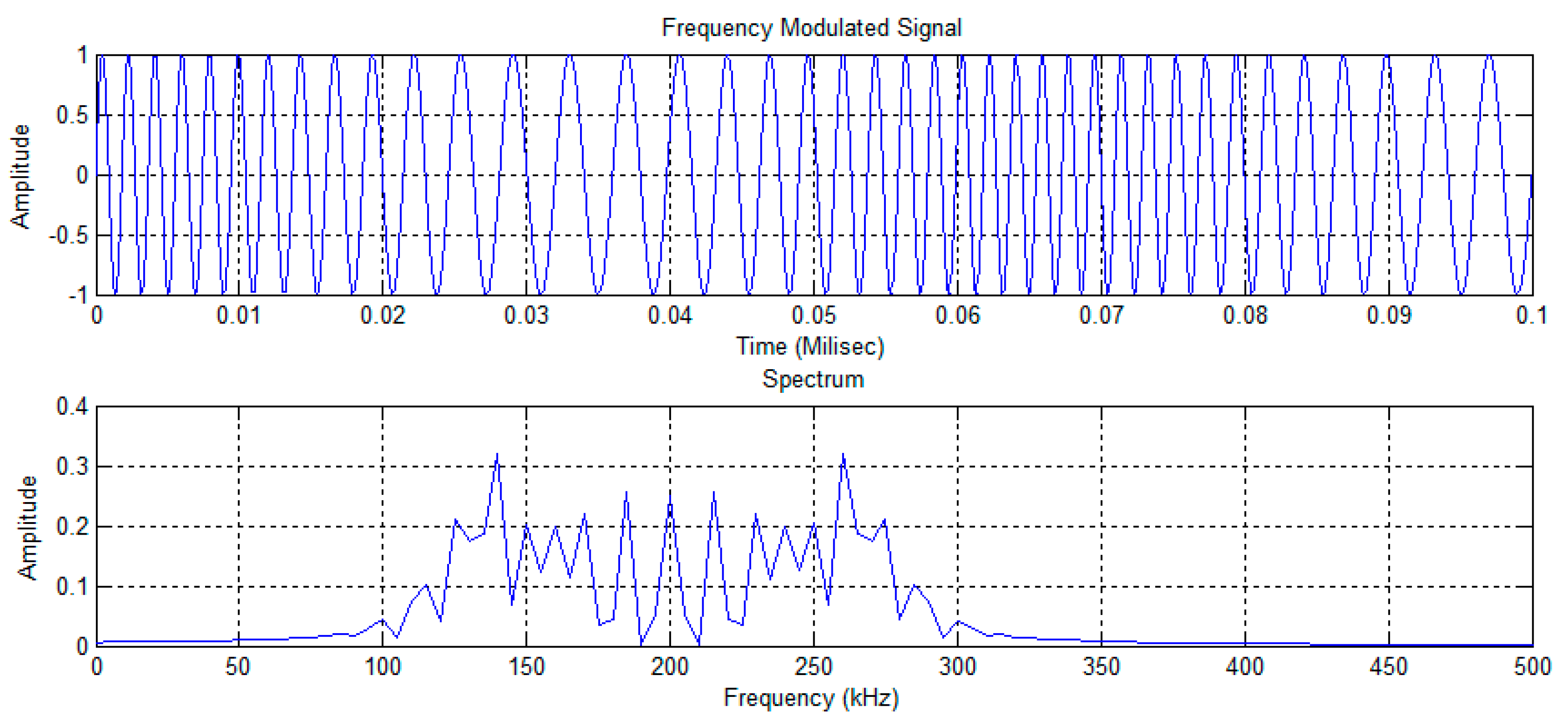
Figure 3.
Example wavelet decomposition of an acousto-ultrasonic (AU) signal using 4 decomposition levels. The raw signal and the four wavelet detail signals as well as the residuals (approximation) are presented.
Figure 3.
Example wavelet decomposition of an acousto-ultrasonic (AU) signal using 4 decomposition levels. The raw signal and the four wavelet detail signals as well as the residuals (approximation) are presented.
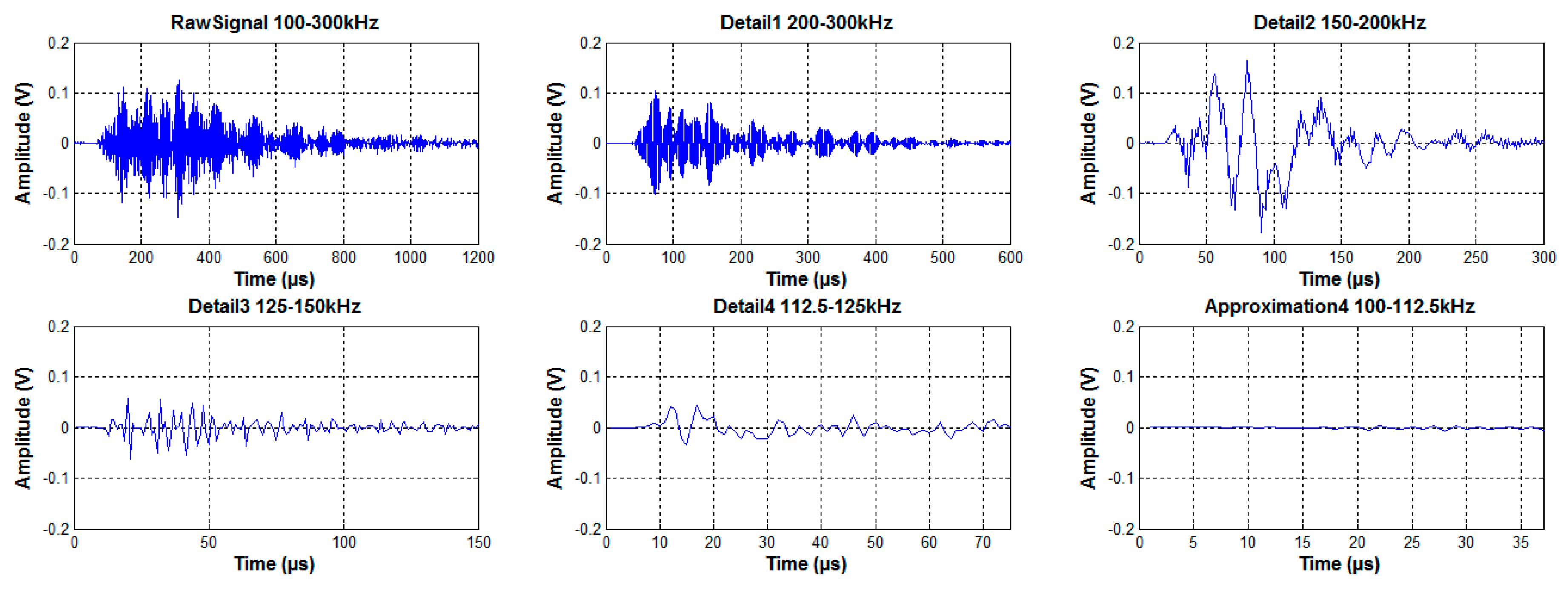
Figure 4.
2D Discrete wavelet decomposition of an X-ray image at four scales and in three directions. The wavelet sub-images are identified by the direction of analysis (h, v, d) followed by the scale number (1–4).
Figure 4.
2D Discrete wavelet decomposition of an X-ray image at four scales and in three directions. The wavelet sub-images are identified by the direction of analysis (h, v, d) followed by the scale number (1–4).

Figure 5.
Score plot of the PCA model (t1–t2) showing the clustering pattern of the corridors in each slice based on their textural features extracted from X-ray images. Observations are identified by the slice number (red numbers in Figure 1) followed by the corridor number (1–6). Different colors are used to distinguish the corridors as shown in the anode slice image included in the figure.
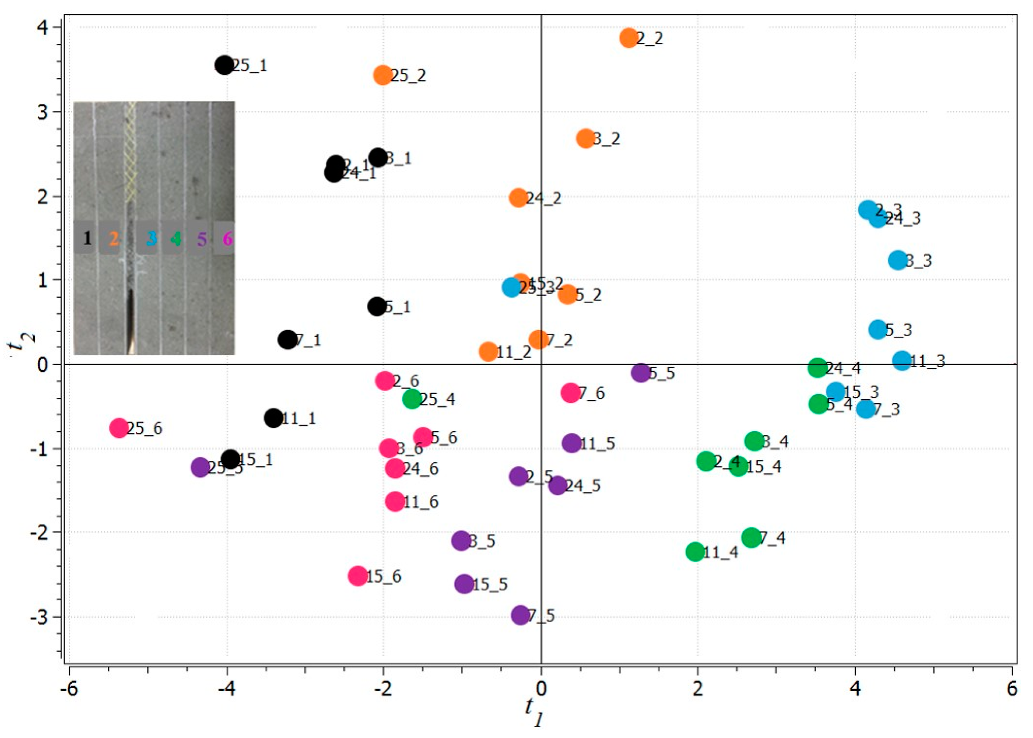
Figure 6.
Loading plot of the PCA model (p1–p2) built on image textural features (Y data). The energy features are identified by letter “E” followed by the wavelet direction (H, V, or D), and scale number.
Figure 6.
Loading plot of the PCA model (p1–p2) built on image textural features (Y data). The energy features are identified by letter “E” followed by the wavelet direction (H, V, or D), and scale number.

Figure 7.
Score plot of the Partial Least Squares (PLS) model (t1–t2) between acoustic attenuation and X-ray image textural features. Observations are identified by the slice number (red numbers in Figure 1) followed by the corridor number (1–6). Different colors are used to distinguish the different corridors as shown in the anode slice image included in the figure.

Figure 8.
Loadings bi-plot (w2*-c1–w2*-c2) of the PLS model between acoustic attenuation signals and X-ray image textural features. The features are identified by their names and by the scale at which they were calculated (1–4).
Figure 8.
Loadings bi-plot (w2*-c1–w2*-c2) of the PLS model between acoustic attenuation signals and X-ray image textural features. The features are identified by their names and by the scale at which they were calculated (1–4).
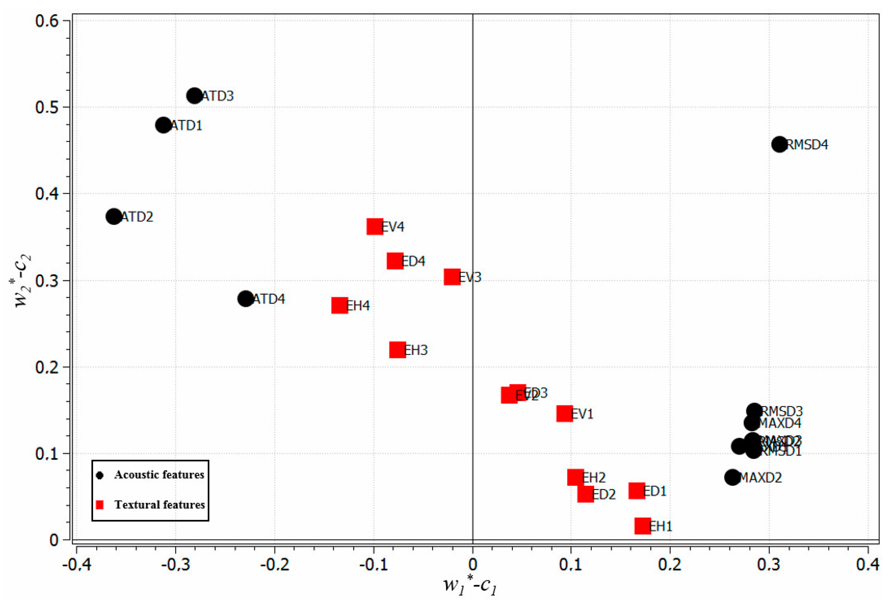
Figure 9.
X-ray images showing the distribution of cracks and pores in selected corridors.

Table 1.
Percent cumulative sum of squares explained (R2) and predicted (Q2) by the Principal Component Analysis (PCA) model built on textural features (Y data) collected from X-ray images of anode slices.
Table 1.
Percent cumulative sum of squares explained (R2) and predicted (Q2) by the Principal Component Analysis (PCA) model built on textural features (Y data) collected from X-ray images of anode slices.
| Component | R2 (%) | Q2 (%) |
|---|---|---|
| 1 | 60.3 | 58.7 |
| 2 | 84.0 | 83.2 |
© 2017 by the authors. Licensee MDPI, Basel, Switzerland. This article is an open access article distributed under the terms and conditions of the Creative Commons Attribution (CC BY) license (http://creativecommons.org/licenses/by/4.0/).
Share and Cite
MDPI and ACS Style
Ben Boubaker, M.; Picard, D.; Duchesne, C.; Tessier, J.; Alamdari, H.; Fafard, M. Inspection of Prebaked Carbon Anodes Using Multi-Spectral Acousto-Ultrasonic Excitation. Metals 2017, 7, 305. https://doi.org/10.3390/met7080305
AMA Style
Ben Boubaker M, Picard D, Duchesne C, Tessier J, Alamdari H, Fafard M. Inspection of Prebaked Carbon Anodes Using Multi-Spectral Acousto-Ultrasonic Excitation. Metals. 2017; 7(8):305. https://doi.org/10.3390/met7080305
Chicago/Turabian StyleBen Boubaker, Moez, Donald Picard, Carl Duchesne, Jayson Tessier, Houshang Alamdari, and Mario Fafard. 2017. "Inspection of Prebaked Carbon Anodes Using Multi-Spectral Acousto-Ultrasonic Excitation" Metals 7, no. 8: 305. https://doi.org/10.3390/met7080305
Note that from the first issue of 2016, this journal uses article numbers instead of page numbers. See further details here.