FEM Simulation of Dissimilar Aluminum Titanium Fiber Laser Welding Using 2D and 3D Gaussian Heat Sources


1
Innovation Engineering Department, University of Salento, Via per Arnesano s.n., 73100 Lecce, Italy
2
DMMM Politecnico di Bari, Viale Japigia, 182, 70126 Bari, Italy
*
Author to whom correspondence should be addressed.
Metals 2017, 7(8), 307; https://doi.org/10.3390/met7080307
Submission received: 1 June 2017
/
Revised: 2 August 2017
/
Accepted: 8 August 2017
/
Published: 10 August 2017
(This article belongs to the Special Issue Laser Welding)
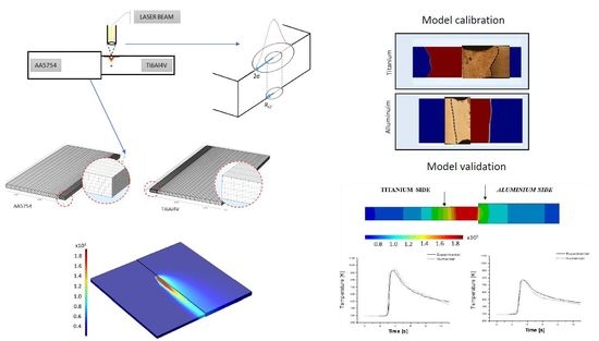
Abstract
:For a dissimilar laser weld, the model of the heat source is a paramount boundary condition for the prediction of the thermal phenomena, which occur during the welding cycle. In this paper, both two-dimensional (2D) and three-dimensional (3D) Gaussian heat sources were studied for the thermal analysis of the fiber laser welding of titanium and aluminum dissimilar butt joint. The models were calibrated comparing the fusion zone of the experiment with that of the numerical model. The actual temperature during the welding cycle was registered by a thermocouple and used for validation of the numerical model. When it came to calculate the fusion zone dimensions in the transversal section, the 2D heat source showed more accurate results. The 3D heat source provided better results for the simulated weld pool and cooling rate.
1. Introduction
Laser welding is recognized as an effective process to weld metals with a laser beam of high-power, high-energy density. In fact, the power density of a laser beam is much higher than that of arc or plasma. Consequently, a deep narrow penetration weld can be effectively produced. These properties have made laser welding a suitable technology for weldments that are made from metals of different compositions and properties [1,2]. A dissimilar joint is as strong as the weaker of the two metals being joined, i.e., possesses sufficient tensile strength and ductility so that the joint will not fail in the weld, has good fatigue behavior [3].
Among them, Al/Ti dissimilar joints are of major interest in aeronautics and automotive applications, where weight reduction, coupled with high mechanical strength and corrosion resistance, are paramount. Between the different Al/Ti welding processes laser welding offers numerous advantages. Especially in aluminum alloys when used in keyhole mode improves the absorption of the beam due to the multiple reflections in the cavity [4]. Moreover, high energy density, high cooling and heating rate allow for reducing the importance of mixing and diffusion phenomena, and thus reduce the formation of intermetallic compounds in the case of dissimilar joints. An Al/Ti joint has a remarkably lower elongation due to the high residual stresses, which facilitate the crack ignition and propagation. Therefore, the quality depends heavily on the process parameters, which determine the magnitude of thermal stresses [5].
The selection of the welding parameters is crucial for obtaining a satisfactory quality weld. Residual stresses and temperature field in laser welding joints can be predicted by numerical analysis such as a finite element one. The Finite Element Method has been one of the performing techniques to predict the joint properties in the welding process, which involves thermal, metallurgical and mechanical phenomena.
The computation of thermal field relies strongly on the heat source model. Rosenthal was the first researcher who proposed a model for the heat source in welding [6]. He proposed an analytical solution considering a punctual or a line heat source. Since then, other more realistic models have been proposed. For arc welding, several heat source configurations have also been proposed. Two and three-dimensional approaches can be used. Zeng et al. described the thermal elastic-plastic analysis using finite element techniques to analyze the thermos-mechanical behavior and evaluate the residual stresses and welding distortion on the AZ31B magnesium alloy and 304L steel butt joint in laser-TIG hybrid welding [7]. A modified three-dimensional conical heat source was used for performing the simulation in arc welding [8,9]. In certain cases, the finite element model is integrated with other computational techniques like artificial intelligence to establish an automated and iterative optimization algorithm [10]. Zeng et al. calculated the thermal cycles and temperature distribution of MIG welding of 5A06 aluminum alloy structure during discontinuous welding. The finite element method transient heat transfer analysis was used to save computing time and improve calculation accuracy [11].
For the fiber laser, Casalino et al. [12] developed and applied a stationary process with a surface heat source model based on thermal load through several specific elements next to the welding line. Other researchers [13] proposed the combination of Gaussian distribution on the surface and distribution along the thickness to consider 3D distribution by applying the conical Gaussian heat source model. They found that 3D conical Gaussian heat distribution can obtain better results with high depth to width ratio (defined as the ratio between the weld penetration evaluated on the axis of fused zone, and the width of the welded seam in the horizontal direction on the sample surface). Nagel et al. [14] proposed some strategies for the optimization of the laser welding of high alloy steel sheets using two different heat sources.
In this paper, two-dimensional and three-dimensional heat distribution was used for welding laser simulation of dissimilar Al/Ti button joint. The objective of this study is to compare the two approaches to establish the best model. The simulated fusion zone was compared with the macrograph obtained from the experiment to calibrate the model. Then, the validation is based on the comparison of the temperature profile measured with thermocouples during the welding cycle.
2. Experimental Setup
A laser butt joint has been produced from two plates of aluminum and titanium (3 and 2 mm, respectively), according to the scheme of Figure 1. Table 1 and Table 2 report the chemical composition of the two alloys and the mechanical and thermo-physical properties at room temperature. Particularly, the thermal conductivity has been considered as a function of temperature (Table 3 and Table 4).
The experimental trials were carried out using an Ytterbium Fiber Laser System (IPG YLS-4000), with a maximum output power equal to 4 kW (IPG Laser, Barbuch, Germany). The laser beam was delivered through a 200 µm optical fiber with a Beam Parameter Product (BPP) equal to 6.3 mm·mrad, the product of a laser beam’s divergence angle (half-angle) and the radius of the beam at its narrowest point. The laser beam, whose wavelength was 1070.6 nm, has been focused continuously through a lens with focal distance of 250 mm producing a spot diameter of 0.4 mm on the workpiece surface. Argon and helium were employed as shielding gas with 10 L/min volumetric flow rate, particularly Argon has been employed on the upper surface and helium on the bottom surface. The laser beam axis was placed on the titanium side, some 1 mm far from the interface (laser offset). The welding parameters have been 1200 W power at 1000 m/min welding rate.
The microstructure of the weld was analyzed by optical microscopy (OM; Nikon Epiphot 200, Nikon, Tokyo, Japan) and Zeiss EVO scanning electron microscope (SEM, Zeiss, Oberkochen, Germany). For optical microscopy observation, the transversal sections of the samples were cut and prepared using the standard metallographic grinding and polishing techniques and attached using Keller reagent (95 mL H2O, 2.5 mL HNO3, 1.5 mL HCl, HF 1 mL). The dimension of the fusion zone (FZ) was evaluated using NIS-Element software (version 4.5, Nikon, Tokio, Japan, 2016)) for the image analysis. NIS-Elements is a Nikon software supplied with Epiphot 200 OM. The software is tailored to facilitate image capture, object measurement and counting. Vickers microhardness profile (0.3/15) was collected using a Vickers Affri Wiky 200JS2 microhardness tester (Affri, Wood Dale, IL, USA) at half of weld cross section thickness. The distance between indentations was equal to 300 μm. The hardness at the Al/Ti fusion zones interface, where an intermetallic compound layer was observed, had been identified with nanoindentation (0.01/15) using Leica VMHT (Leica Microsystems Wetzlar GmbH, Wetzlar Germany) due to the reduced size of the layer.
Two thermocouple recording systems were placed in the middle of the plates, 2 mm distant from the weld centre line in both titanium and aluminum side. The calibration of the two models was carried out by comparing the size and shape of the fusion zone of the numerical model and the experimental one. The validation of the model was made by comparing the experimental and numerical thermal cycle.
3. Numerical Model
3.1. Model for the Plates
The plates of titanium and aluminum (200 mm × 50 mm) were joined along the long side. The plates have different thickness, i.e., 2 mm for titanium one and 3 mm for Aluminum one. The adopted mesh is the same for the two models. To obtain accurate results, a fine mesh was adopted close to the welding line. Mesh size was determined rapidly by trial-and-error; likewise, it is generally done in the literature. Mesh size is equal to 1 × 0.5 × 0.5 mm3 inside of 10 mm from the interface and the number of the nodes is equal to 20 along the x-axis. At a distance from the interface higher than 10 mm, the mesh size increases along the x-axis. Particularly from 10 to 50 mm far from the interface (the limit of the Al sheet), the number of the nodes is equal to 20, but the ratio in size between the last element and first element in the distribution is 0.1 (arithmetic sequence). The mapped mesh has 40,000 elements and 49,692 nodes. Figure 2 shows the results of the meshing procedure.
The numerical simulation was performed using the finite element code COMSOL Multiphysics. Comsol Multiphysics is a Multiphysics modeling tool that solves all types of problems based on Finite Element [15].
During the welding process, the transfer of heat is governed by the general equation heat flow (1a):
where
is the density of the metal as a function of temperature,
[J/(g·K)] is specific heat of the metal as a function of temperature,
[m/s] is the velocity field,
is the heat lost to the surroundings by combination of radiation and convection and conduction,
is the heat source.
The heat lost is given by Equation (1b):
where ε is the emissivity of the surface and is taken as 0.5 for titanium and 0.3 for aluminum. σ is the Stefan–Boltzmann constant and is taken as 5.67 × 10⁻⁸ W/(m2·K4), Tr is the room temperature and was taken at 293 K. h is the heat transfer coefficient assumed equal to 20 W/(m2·K) for air and 200 W/(m2·K) for the bottom surface in contact with the workspace.
When the contact is formed by pressing two similar or dissimilar metallic materials together, only a small fraction of the nominal surface area is in contact because of the roughness and irregularities of the contacting surfaces. When a heat flux is imposed across the junction, there are only a limited number and size of the contact spots that results in an actual contact area. The actual contact area is significantly smaller than the apparent contact area and causes a thermal contact resistance. There are several analytic expressions for predicting the contact conductance, and several values in literature [16]. Based on these values, by acting on a contact resistance value, the calibration has been carried out by comparing the fusion zones of the numerical model with the experimental results. Finally, the value of contact conductance is assumed to be equal to 30,000 W/(m2·K), for both of the two models [17]. Mechanical constraints were imposed for the simulation of the clamping system. Constraints were imposed to the four exterior nodes of the plates so degrees of freedom were zero (no displacement is permitted).
3.2. 2D Heat Source
Since the pioneering work of Rosenthal [6] that proposed punctual and linear heat sources, several more realistic sources have been proposed. When the distribution along the thickness is not important like in thin plates, the surface Gaussian heat source model is a good proposal for bed-on-plate cases when both TIG and conductive laser welding must be simulated [18]. For the surface laser heat source, the radius should be calculated first by the formula written as [19]:
where is the beam quality equal to 1.1 for fiber laser, is the focal length of the focusing lens and is the diameter of the lens.
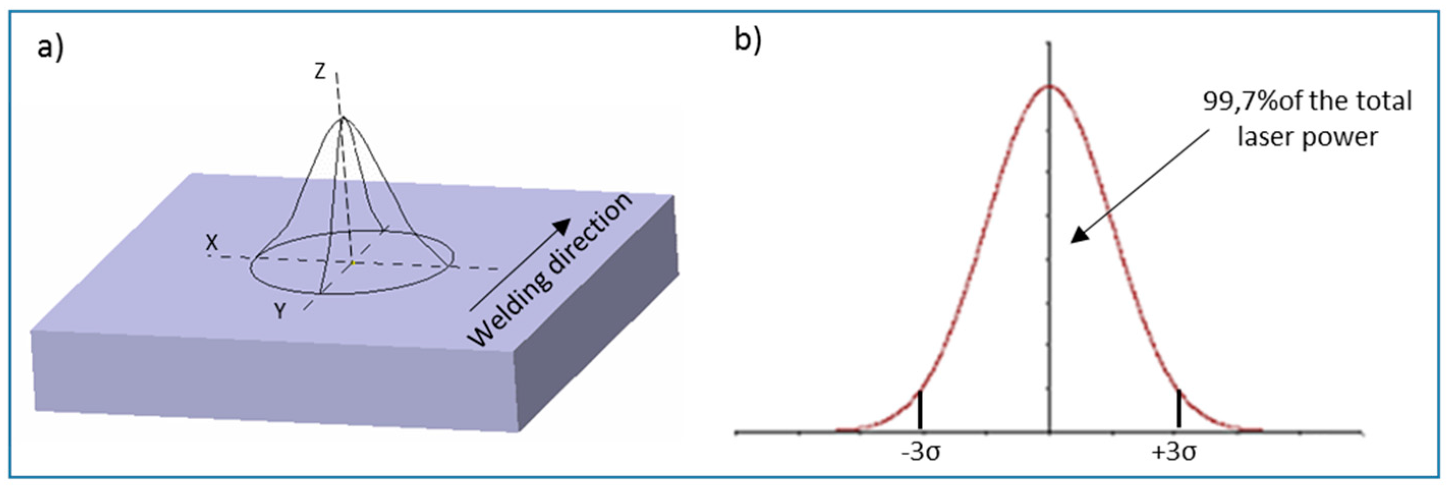
For laser welding, the heat source of the laser beam was simulated by a traveling two-dimensional distribution of heat source (Figure 3a). Particularly, the heat surface distribution was built by combining two Gaussian distributions one in the plane XZ and one moving with welding rate in plane YZ. Those two Gaussian distributions were obtained, and, with an energy of about 99.7% of the total laser energy, a fusion of the titanium alloys was obtained. The heat source radius was assumed equal to three standard deviations of the Gaussian pulse (Figure 3b):
The 2D total heat source (W) (Figure 4) is expressed in Equation (4):
3.3. 3D Heat Source
For the three-dimensions laser source, the heat flux was described in the numerical model as a volume and surface distributed heat flux:
where the coefficient is the energy fraction that will be introduced through the cylinder, and the remaining energy will be introduced via the surface heat source (the value being used is 0.9).
For the surface, a Gaussian distribution was used, the heat source radius was equal to two standard deviations of the Gaussian pulse under the assumption that 95.44% of the total fusion energy of the titanium alloys was applied. In this case, considering the surface heat distribution proposed by Goldak and Akhlagi [20], the surface heat flux [W/mm2] can be expressed as shown in Equation (6):
where is the process efficiency (the value being used is 1), is the laser power in W and is the heat source radius.
For volume heat source, a constant heat distribution cylinder was considering, with a radius equal to those of the molten cylinder (Figure 5). The numeric value for volumetric heat source is given by the ratio between the laser power and the volume of cylinder with a radius .
Thus, finally, the keyhole is modelled in the software using the heat source radius, the radius of the molten cylinder, measured by experimental results, and the energy fraction.
4. Results and Discussion
4.1. Metallurgical Characterization of Weld
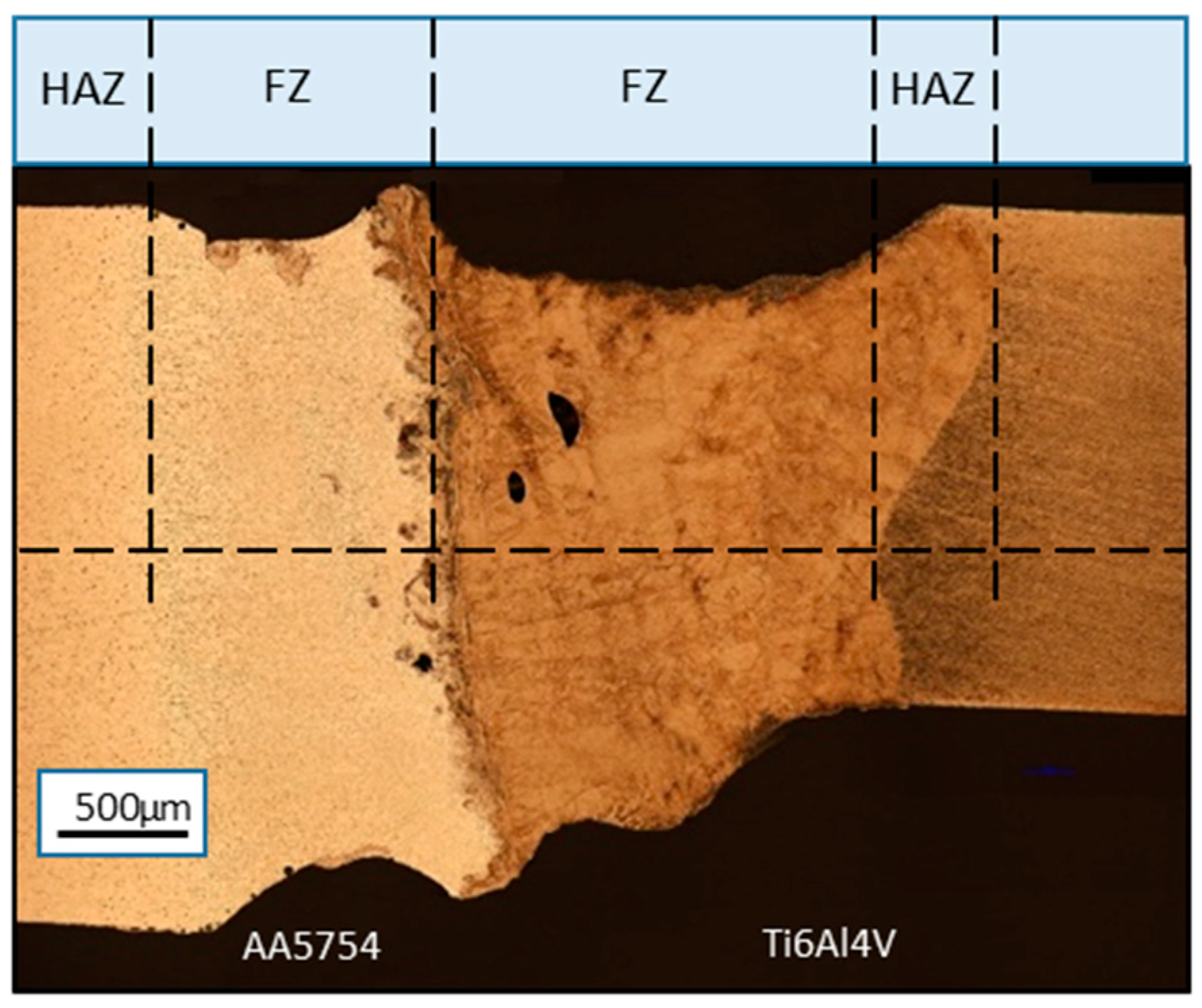
The appearance of Ti6Al4V/AA5754 laser welded joint after chemical etching is shown in Figure 6. Both titanium and aluminum alloy melted at the joint interface and separate fusion zones were observed (Al side and Ti side) as well as two heat affected zone (HAZ) between FZ and the base material. Good weld appearance of the cross section was obtained with full penetration and low level of porosity. It was demonstrated that in aluminum-titanium dissimilar weld, porosity tended to be produced in the fusion line. It happens that gases in the seam are hard to escape and concentrated in the middle of fusion line during the solidification process [21]. In Figure 6, some gas trapping occurred on both sides of the intermetallic layer but not in the intermetallic layer.
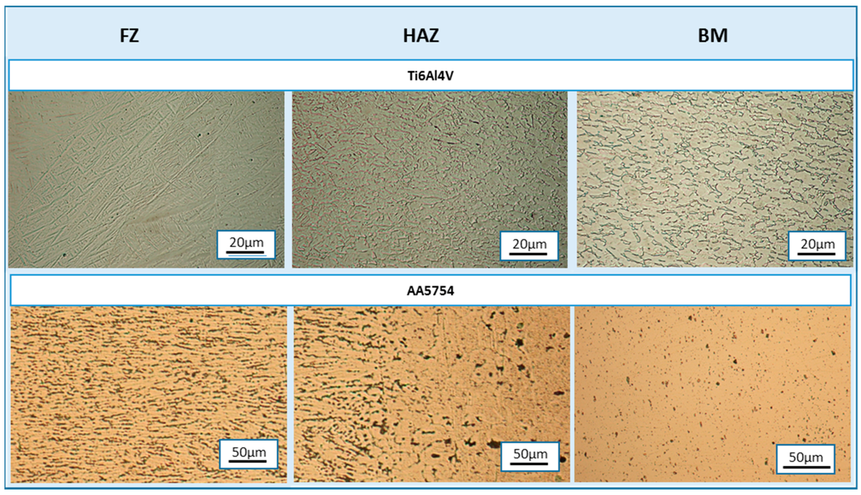
Figure 7 shows the Ti microstructure of the different zones showed in Figure 6, i.e., base material, heat affected zone and fusion zone. The basic mental (BM) is composed of dark β phase in the dominating bright α matrix. Particularly, the β phase is distributed at the boundary of the α grains. This is a typical microstructure for α-β titanium alloys in mill-annealed conditions [22]. The microstructure within the joint depends on the heat received from the laser beam, and varies according to the distance from it. In FZ, a predominantly martensitic microstructure of acicular type (α’) is present. In fact, as reported in literature [22,23,24], the microstructure of the laser fusion zone of Ti-6Al-4V alloy is completely martensitic due to the high cooling speed from β field. The heat affected zone is a mixture of martensitic and primary α grain. During the heat thermal cycle due to the laser heating, an increase of β phase results. However, due to the rapid cooling, that transformation is never complete, so the microstructure of the HAZ is mixed, formed from martensitic grains and grain α.
The base material aluminum alloy AA5754 was supplied in the annealed condition (Figure 7). In the aluminum matrix, there are some second phases. These phases have been identified in literature as (Fe,Mn)Al6, (Fe,Mn)3SiAl12, Mg2Si and Mg2Al3 [25,26,27].
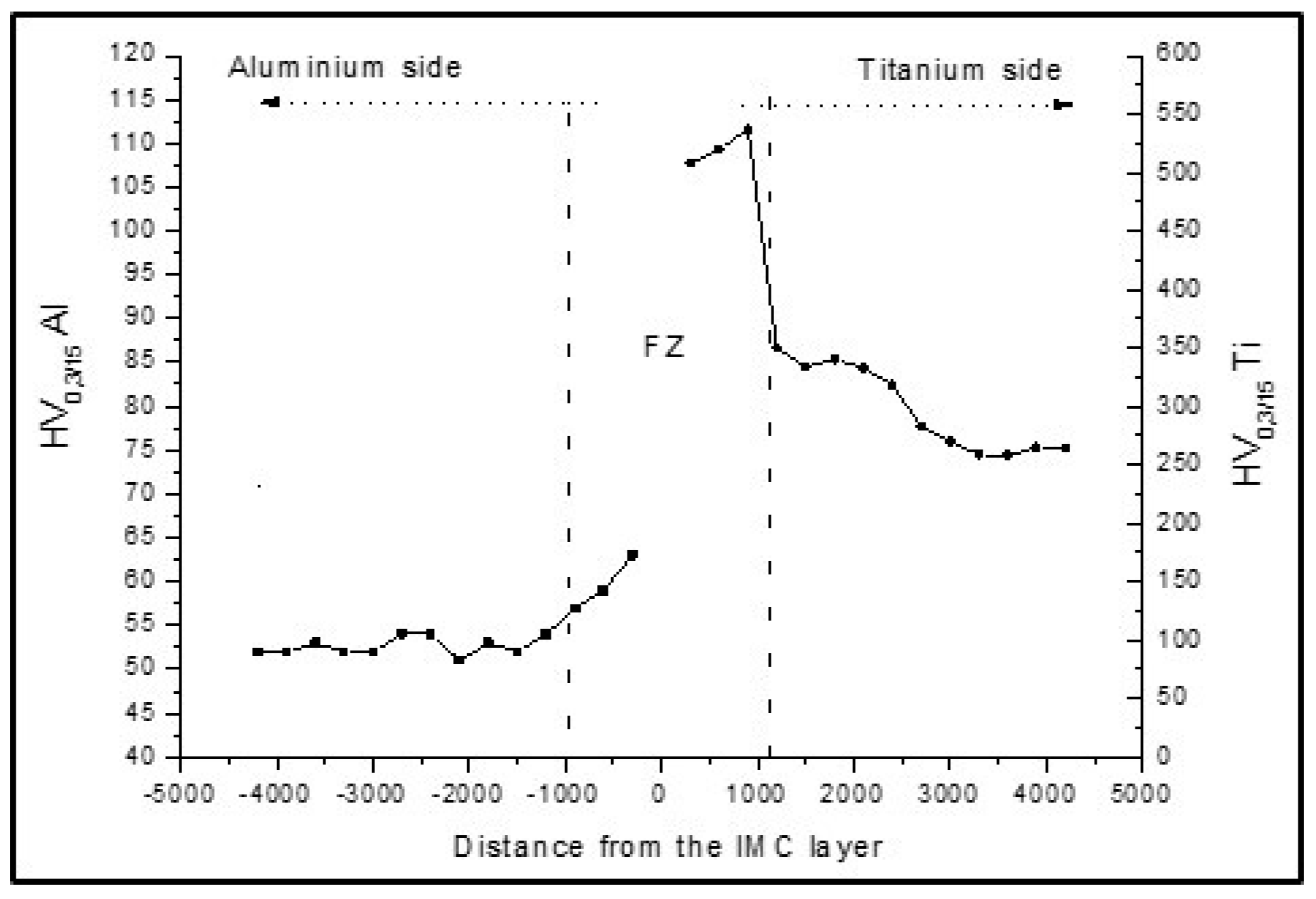
The microstructure of the fusion zone exhibits a very fine dendritic microstructure due to the high cooling rate. The dendrites grow in direction parallel to the direction of heat flow giving to columnar grains [28,29]. In the HAZ microstructure, no detectable changes are evident to the OM; however, in this zone, solubilization of magnesium based has been reported in the literature [30]. Figure 8 shows the micro hardness profile (0.3/15) in the transverse section of the weld. The microhardness was very high in the titanium FZ where the microstructure was martensitic. In the HAZ, the value diminished with the lower amount of martensitic microstructure. The rise in the microhardness of the FZ of aluminum in the weld was caused by the rapid cooling that produced a very fine solidification structure and solid solution strength. The increment in the HAZ of aluminum was due to the dissolution of magnesium compounds during the welding cycle [30].
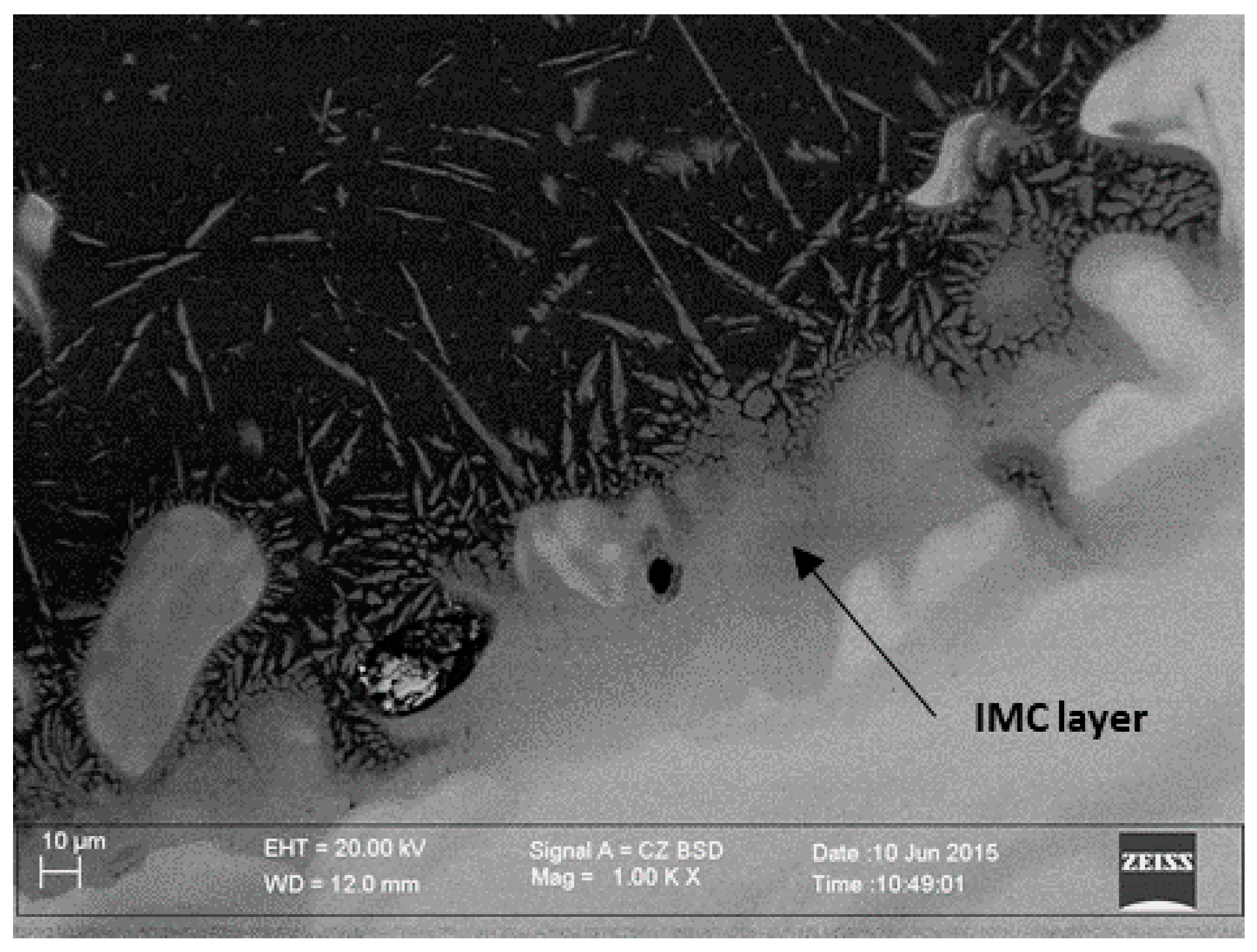
A layer of intermetallic compounds (IMC) formed between the two fusion zones (Figure 9), whose stoichiometry was clarified in some paper [26,31,32]. This layer is due to the reaction in the temperature of the two alloys, and the size is variable as a function of the process parameters [32]. Particularly for the welding process parameters concerning this study, the average thickness of the IMC layer was equal 50 ± 5 µm to and the average nanohardness value (0.01/15) was equal to 2485 ± 232.
4.2. Calibration of the Model
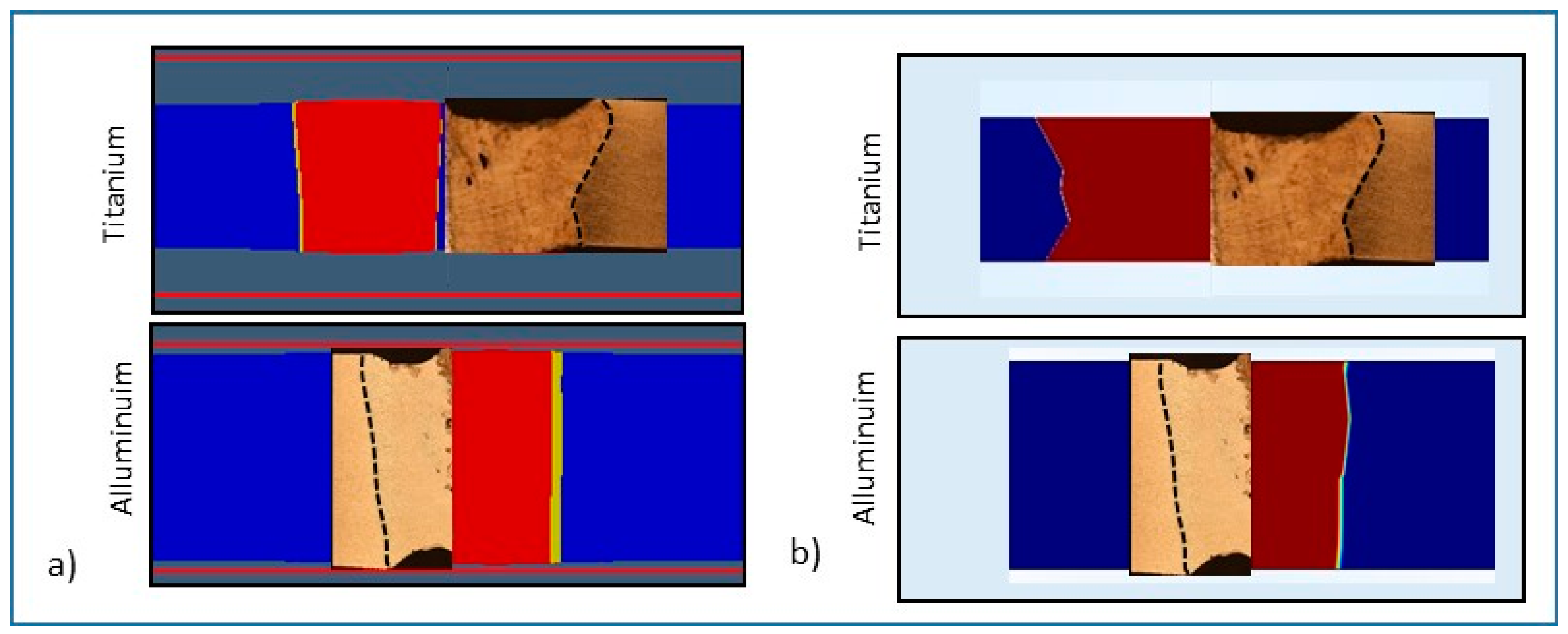
After the simulation, the fusion zone was compared with the experimental one for calibration purposes. Figure 10 shows the comparison between the simulated and experimental fusion zone profile for aluminum and titanium. For both 2D and 3D heat source modeling, a complete penetration of keyhole was obtained, and, particularly for the 2D heat source, the boundary of the fusion zone obtained numerically had similar shapes in comparison with the experimental ones.
In Table 5 and Table 6, the dimensions of the fusion zone profile, respectively, in the top, middle and bottom, are reported both for 2D and 3D numerical simulation and the experimental measure. A better matching between the numerical and experimental results for the size of fusion zone has been obtained using a 2D source.
In fact, by correctly adjusting keyhole parameter in 3D heat source, only the top width of the weld was close to the experimental result, while the 2D heat source could almost precisely calculate the top, middle and bottom width. The observed performance can be explained as follows. It is well known that the behavior of heat flow depends on welding conditions [14,33]. For higher welding powers and thinner plates, the heat flow is predominantly 2D, whereas for lower welding powers and thicker plates, the heat flow was 3D. Therefore, there must be a transition thickness in which the heat flow has a behavior, which is a mix of the 2D and 3D ones. Probably for the thin plates examined in this study, the heat flow was predominantly 2D, and that is why 2D heat flow modelling is more appropriate.
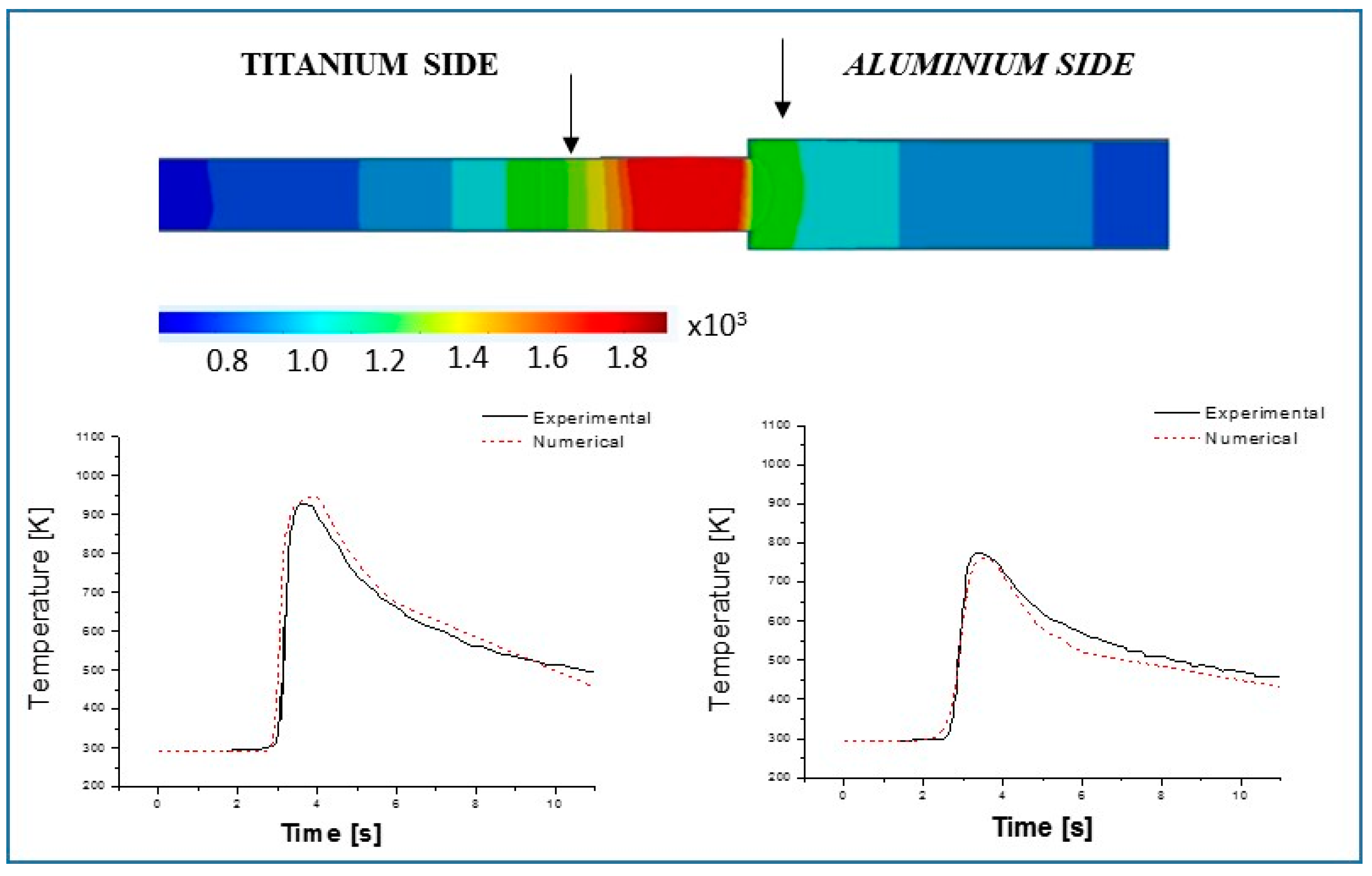
Figure 11 and Figure 12 show the temperature distribution on the top when the weld bead profile reached the quasi-steady state. The thermal conductivity of the two materials influenced the position of the maximum temperature in the melt pool and away from the melt pool. For both numeric simulation, the maximum temperature was recorded within the titanium side, where the beam laser was directed. The width of the heat affected zone in the aluminum side was greater due to the high thermal conductivity of the aluminum alloy. On the contrary, the low thermal conductivity of the titanium alloy leads to accumulating the heat over the metal by reducing the area interested from metallurgical transformation.
The shape of the weld pool longitudinal plane (Figure 13) showed a teardrop shape for the 2D heat source. Thus, this means that probably the 2D heat source cannot perfectly simulate the laser heat source. However, better results have been obtained using the 3D heat source; in this case, the resulting molten puddle had an elliptical shape, which is more similar to the experimental pool shape as shown by microstructure evolution of the grains (Figure 14) in the fusion zone. This shape of the grains derives from the elliptical molten pool [24,34].
4.3. Validation of the Model
The temperature cycle was measured in two different points that were placed 2 mm away from the weld centerline on both sides of the weld (Figure 15 and Figure 16). The temperature profiles were compared with those obtained from the thermocouples. High thermal gradients, and fast cooling rate were present, due to the laser process. When it concerns the temperature peak, the numerical results matched the experimental one for both of the heat sources. Nonetheless, regarding the cooling rate, the 3D heat source was more precise than the 2D one.
5. Conclusions
In this paper, the numerical models to simulate the laser welding process of butt dissimilar Al/TI joints were developed. Two different 2D and 3D heat source modelling processes have been utilized to simulate the proper heat flux during the welding. The numeric results were compared with the experimental ones to calibrate and to validate the two models. The metallurgical analyses showed that the titanium fusion zone was principally martensitic, and the heat affected zone was a mixture of martensitic and primary α grain. In the aluminum fusion zone, a dendritic structure was present and the heat affected zone was characterized by the solubilization of the magnesium compounds.
The FEM simulation of the thermal cycle of fiber offset welding was satisfactory. The following points were demonstrated:
- (1)
- The calculations for the fusion zone dimensions were accurate both for the 2D and the 3D heat source. By using that 2D heat source, a better matching of numeric and experimental results was obtained at the three levels at which the molten zone sizes were taken.
- (2)
- In the longitudinal section, the numerical results were not as accurate for both of the heat sources. For the 2D one, a teardrop shape of the molten weld pool formed while the 3D heat source produced an elliptical one. It is possible to conclude that the 3D heat source can better approximate the heat flux during laser welding and the maximum temperature gradients, which determined the change in the grain growth direction in the titanium side.
- (3)
- The overall thermal cycle accuracy was good for 2D and 3D heat sources. However, the 3D heat source provided better results for the cooling rate simulation.
Author Contributions
The welds were fabricated in the TISMA ((Innovative Welding for Advanced Materials) laboratory of Bari, which is led by Giuseppe Casalino. Paola Leo looked after the metallographic preparation and analysis of the microstructure and Sonia D’Ostuni built the numerical model. Discussion and conclusions were written with the contribution of all authors.
Conflicts of Interest
The authors declare no conflict of interest.
References
- Oliveira, J.P.; Zeng, Z.; Andrei, C.; Braz Fernandes, F.M.; Miranda, R.M.; Ramirez, A.J.; Omori, T.; Zhou, N. Dissimilar laser welding of superelastic NiTi and CuAlMn shape memory alloys. Mater. Des. 2017, 128, 166–175. [Google Scholar] [CrossRef]
- Casalino, G.; Guglielmi, P.; Lorusso, V.D.; Mortello, M.; Peyre, P.; Sorgente, D. Laser offset welding of AZ31B magnesium alloy to 316 stainless steel. J. Mater. Process. Technol. 2017, 242, 49–59. [Google Scholar] [CrossRef]
- Zeng, X.; Oliveira, J.P.; Yang, M.; Song, D.; Peng, B. Functional fatigue behavior of NiTi-Cu dissimilar laser welds. Mater. Des. 2017, 114, 282–287. [Google Scholar] [CrossRef]
- Katayama, S. Handbook of Laser Welding Technologies; Woodhead Publishing Limited: Sawston, UK, 2013. [Google Scholar]
- Casalino, G.; Mortello, M.; Peyre, P. Yb–YAG laser offset welding of AA5754 and T40 butt joint. J. Mater. Process. Technol. 2015, 223, 139–149. [Google Scholar] [CrossRef]
- Rosenthal, D. Mathematical theory of heat distribution during welding and cutting. Weld. J. 1941, 20, 220–234. [Google Scholar]
- Zeng, Z.; Li, X.; Miao, Y.; Wu, G.; Zhao, Z. Numerical and experiment analysis of residual stress on magnesium alloy and steel butt joint by hybrid laser-TIG welding. Comput. Mater. Sci. 2011, 50, 1763–1769. [Google Scholar] [CrossRef]
- Pham, S.M.; Tran, V.P. Study on the Structure Deformation in the Process of Gas Metal Arc Welding (GMAW). Am. J. Mech. Eng. 2014, 2, 120–124. [Google Scholar]
- Dhinakaran, V.; Suraj Khope, N.S.S.; Sankaranarayanasamy, K. Numerical Prediction of Weld Bead Geometry in Plasma Arc Welding of Titanium Sheets Using COMSOL. In Proceedings of the 2014 COMSOL Conference in Bangalore, Bangalore, India, 13–14 October 2014. [Google Scholar]
- Casalino, G.; Hu, S.J.; Hou, W. Deformation prediction and quality evaluation of the gas metal arc welding butt weld. Proc. Inst. Mech. Eng. Part B 2003, 217, 1615–1622. [Google Scholar] [CrossRef]
- Zeng, Z.; Wang, L.; Wang, Y.; Zhang, H. Numerical and experimental investigation on temperature distribution of the discontinuous welding. Comput. Mater. Sci. 2009, 44, 1153–1162. [Google Scholar] [CrossRef]
- Casalino, G.; Michelangelo, M. A FEM model to study the fiber laser welding of Ti6Al4V thin sheets. Int. J. Adv. Manuf. Technol. 2016, 86, 1339–1346. [Google Scholar] [CrossRef]
- Azizpour, M.; Ghoreishi, M.; Khorram, A. Numerical simulation of laser beam welding of Ti6Al4V sheet. J. Comput. Appl. Res. Mech. Eng. 2015, 4, 145–154. [Google Scholar]
- Falk, N.; Flaviu, S.; Benjamin, K.; Jean, P.B.; Jorg, H. Optimization strategies for laser welding high alloy steel sheets. Phys. Proced. 2014, 56, 1242–1251. [Google Scholar]
- Comsol Multiphysics, version 5.2a; Software for Multiphysics Modeling; COMSOL: Stockholm, Sweden, 2016.
- Contuzzi, N.; Campanelli, S.L.; Casalino, G.; Ludovico, A.D. On the role of the Thermal Contact Conductance during the Friction Stir Welding of an AA5754-H111 butt joint. Appl. Therm. Eng. 2016, 104, 263–273. [Google Scholar] [CrossRef]
- Casalino, G.; Mortello, M.; Peyre, P. FEM Analysis of Fiber Laser Welding of Titanium and Aluminum. Procedia CIRP 2016, 41, 992–997. [Google Scholar] [CrossRef]
- Teixeira, P.R.D.F.; Araújo, D.B.D.; Cunda, L.A.B.D. Study of the gaussian distribution heat source model applied to numerical thermal simulations of tig welding processes. Ciênc. Eng. 2014, 23, 115–122. [Google Scholar] [CrossRef]
- Steen, W.M.; Mazumder, J. Laser Material Processing; Springer: Berlin, Germany, 2010. [Google Scholar]
- Goldak, J.; Akhlagi, M. Computational Welding Mechanics; Springer: Ottawa, ON, Canada, 2005; pp. 26–27. [Google Scholar]
- Lv, S.X.; Jing, X.J.; Huang, Y.X.; Xu, Y.Q.; Zheng, C.Q.; Yang, S.Q. Investigation on TIG arc welding–brazing of Ti/Al dissimilar alloys with Al based fillers. Sci. Technol. Weld. Join. 2012, 17, 519–524. [Google Scholar] [CrossRef]
- Lutjering, G.; Williams, J.C. Titanium (Engineering Materials and Processes), 2nd ed.; Springer: Berlin, Germany; New York, NY, USA, 2007. [Google Scholar]
- Akman, E.; Demir, A.; Canel, T.; Sınmazcelik, T. Laser welding of Ti6Al4V titanium alloys. J. Mater. Process. Technol. 2009, 209, 3705–3713. [Google Scholar] [CrossRef]
- Xu, P.; Li, L.; Zhang, C. Microstructure characterization of laser welded Ti-6Al-4V fusion zones. Mater. Charact. 2014, 87, 179–185. [Google Scholar] [CrossRef]
- Kumar, S.; Nadendla, H.B.; Scamans, G.M.; Eskin, D.G.; Fan, Z. Solidification behavior of an AA5754 alloy ingot cast with high impurity content. Int. J. Mater. Res. 2012, 103, E1–E7. [Google Scholar] [CrossRef]
- Raghavan, V. Phase Diagram Evaluations: Section II. J. Ph. Equilib. Diffus. 2005, 26, 171–172. [Google Scholar] [CrossRef]
- ASM Specialty Handbook: Aluminum and Aluminum Alloys; Davis, J.R. (Ed.) ASM International: Novelty, OH, USA, 1993. [Google Scholar]
- Porter, D.A.; Easterling, K.E. Phase Transformations in Metals and Alloys; Chapman & Hall: London, UK, 1992. [Google Scholar]
- Verhoeven, J.D. Fundamentals of Physical Metallurgy; Wiley: Hoboken, NJ, USA, 1975. [Google Scholar]
- Leo, P.; D’Ostuni, S.; Casalino, G. Hybrid welding of AA5754 annealed alloy: Role of post weld heat treatment on microstructure and mechanical properties. Mater. Des. 2016, 90, 777–786. [Google Scholar] [CrossRef]
- Bailey, N. Welding Dissimilar Metals; The Welding Institute: Cambridge, UK, 1986. [Google Scholar]
- Gao, M.; Chen, C.; Gu, Y.; Zeng, X. Microstructure and tensile behavior of laser arc hybrid welded dissimilar Al and Ti alloys. Materials 2014, 7, 1590–1602. [Google Scholar] [CrossRef]
- Sorensen, M.B. Simulation of Welding Distortion in Ship Section. Ph.D. Thesis, University of Denmark, Lyngby, Denmark, 1999. [Google Scholar]
- Messler, R.W. Principles of Welding; Wiley-VCH, John Wiley & Sons, Inc.: Singapore, 2004. [Google Scholar]
Figure 1.
Scheme of laser welding on AA5754/Ti6Al4V.
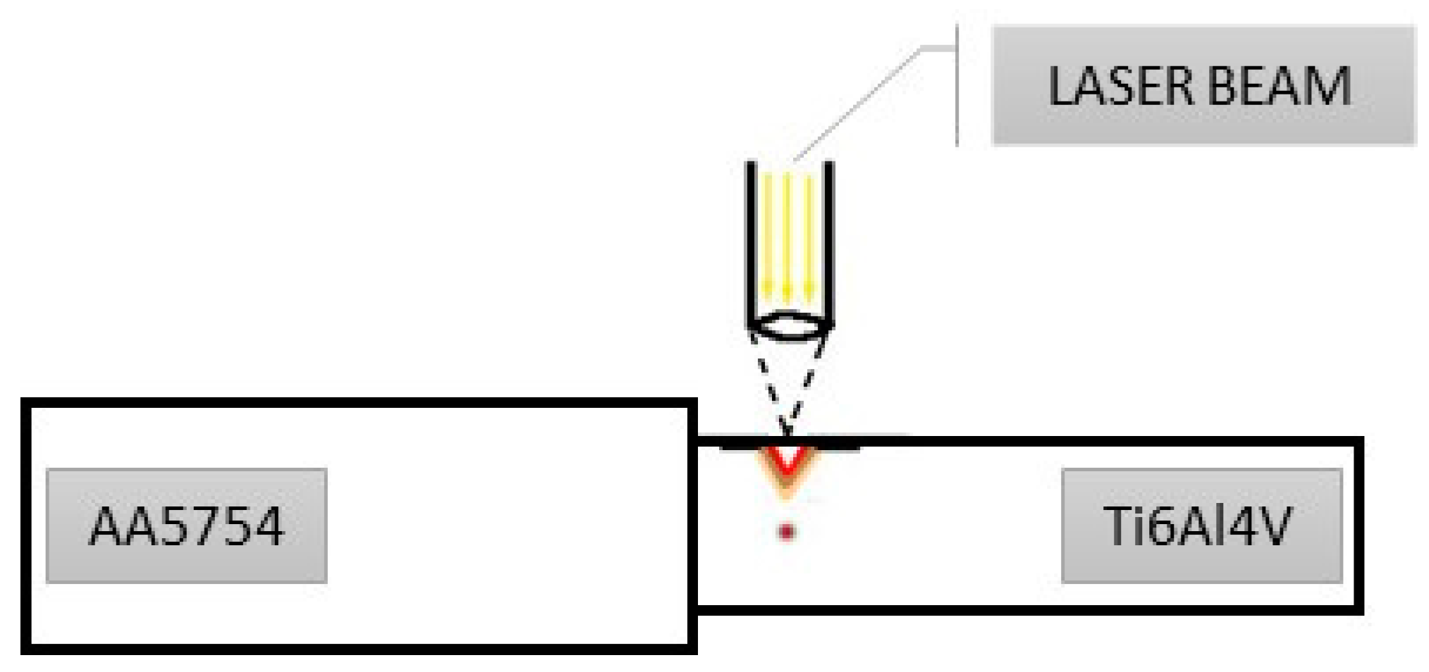
Figure 2.
Mesh outlook.

Figure 3.
(a) Combining of the two Gaussian distribution in plane XZ and XY, and (b) Gaussian distribution.
Figure 3.
(a) Combining of the two Gaussian distribution in plane XZ and XY, and (b) Gaussian distribution.

Figure 4.
Heat flux in 2D Gaussian heat distribution.
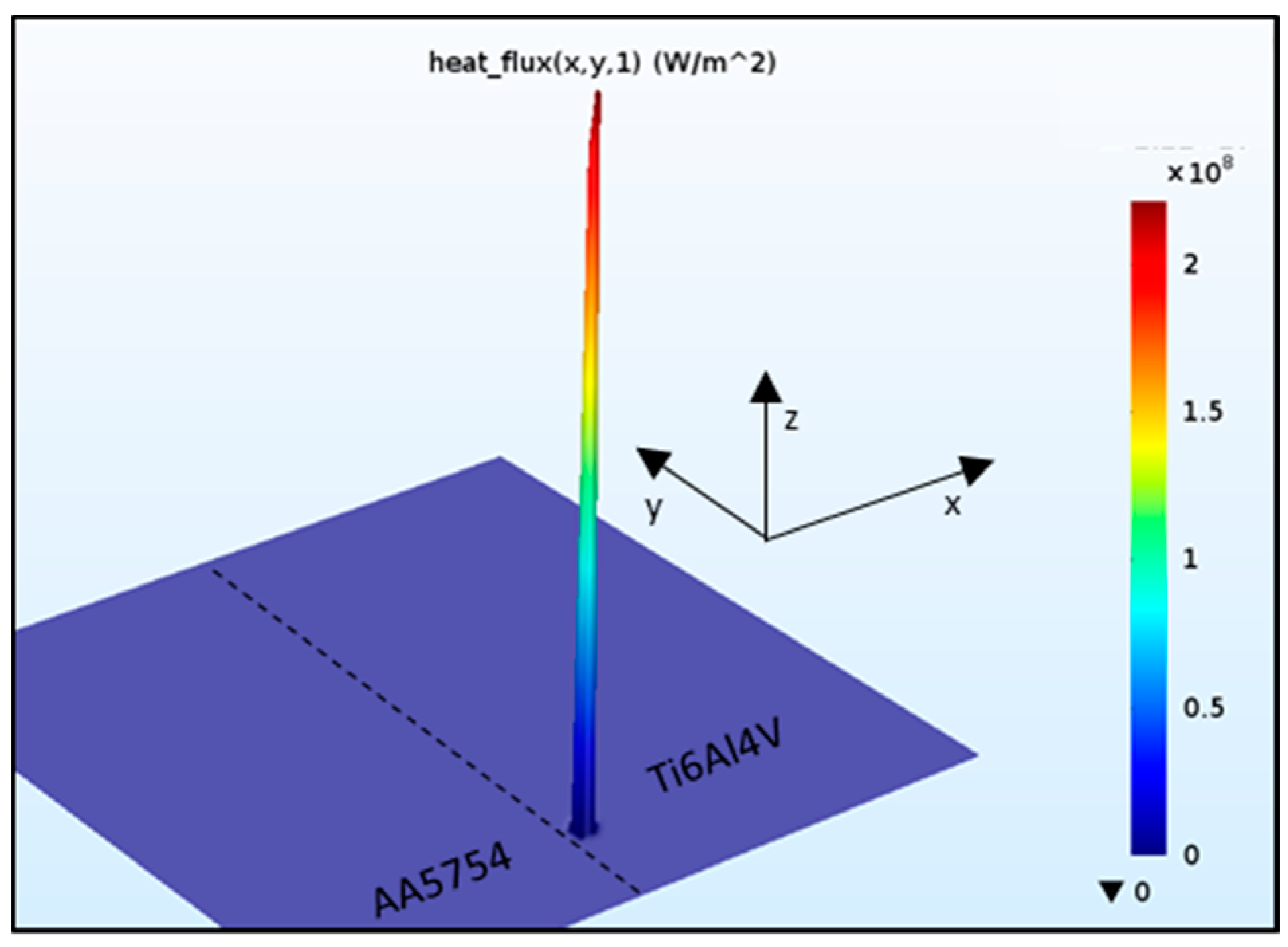
Figure 5.
Total heat flux in 3D heat distribution.
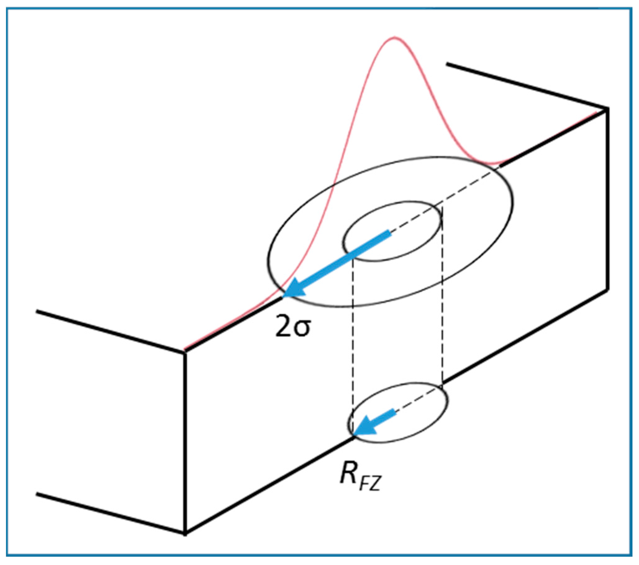
Figure 6.
Appearance of Ti6Al4V/AA5754 laser welded joint after chemical etching.

Figure 7.
Microstructure of the various zones in Ti6Al4V and AA5754.

Figure 8.
Microhardness profile at half thickness of the weld cross section.

Figure 9.
SEM Micrograph of intermetallic compounds (IMC) layer at the Al/Ti joint interface.

Figure 10.
Calibration of (a) 3D and (b) 2D heat source models by the cross section of the weld.

Figure 11.
Isometric view of temperature distributions (in Kelvin) using 2D heat source modelling.
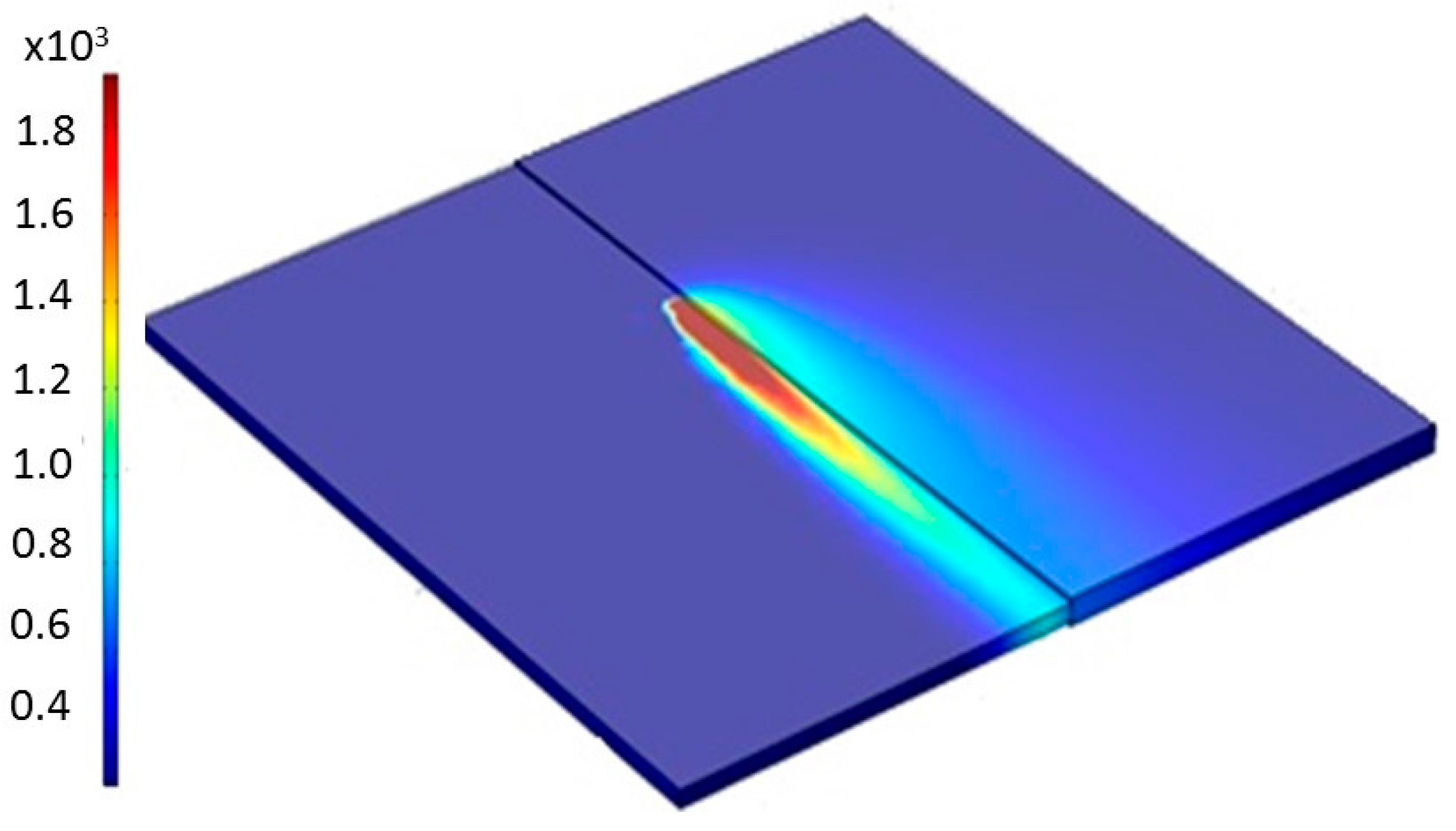
Figure 12.
Isometric view of temperature distributions (in Kelvin) using 3D heat source modelling.
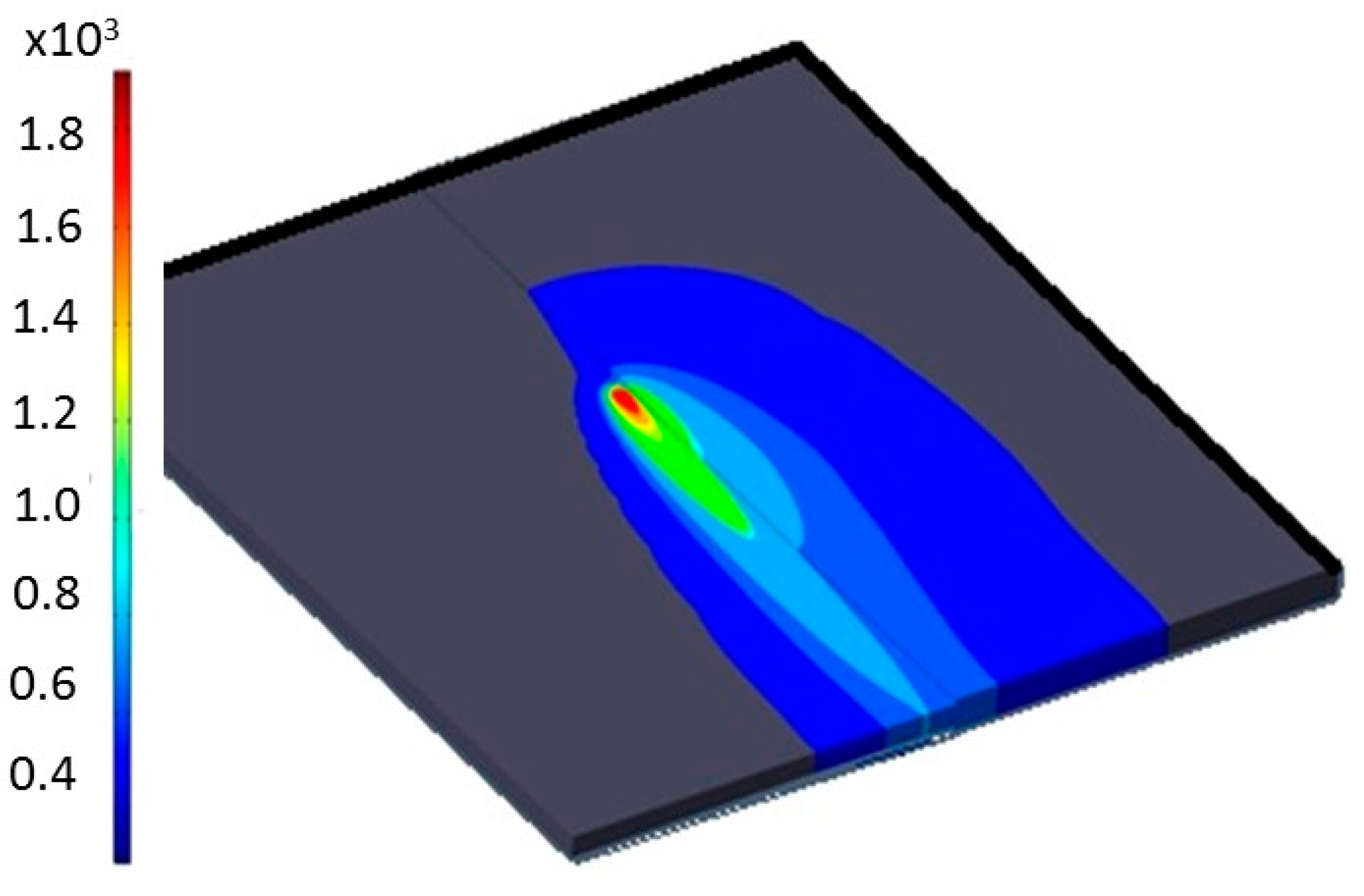
Figure 13.
Weld pool numerical results for the numerical simulations.
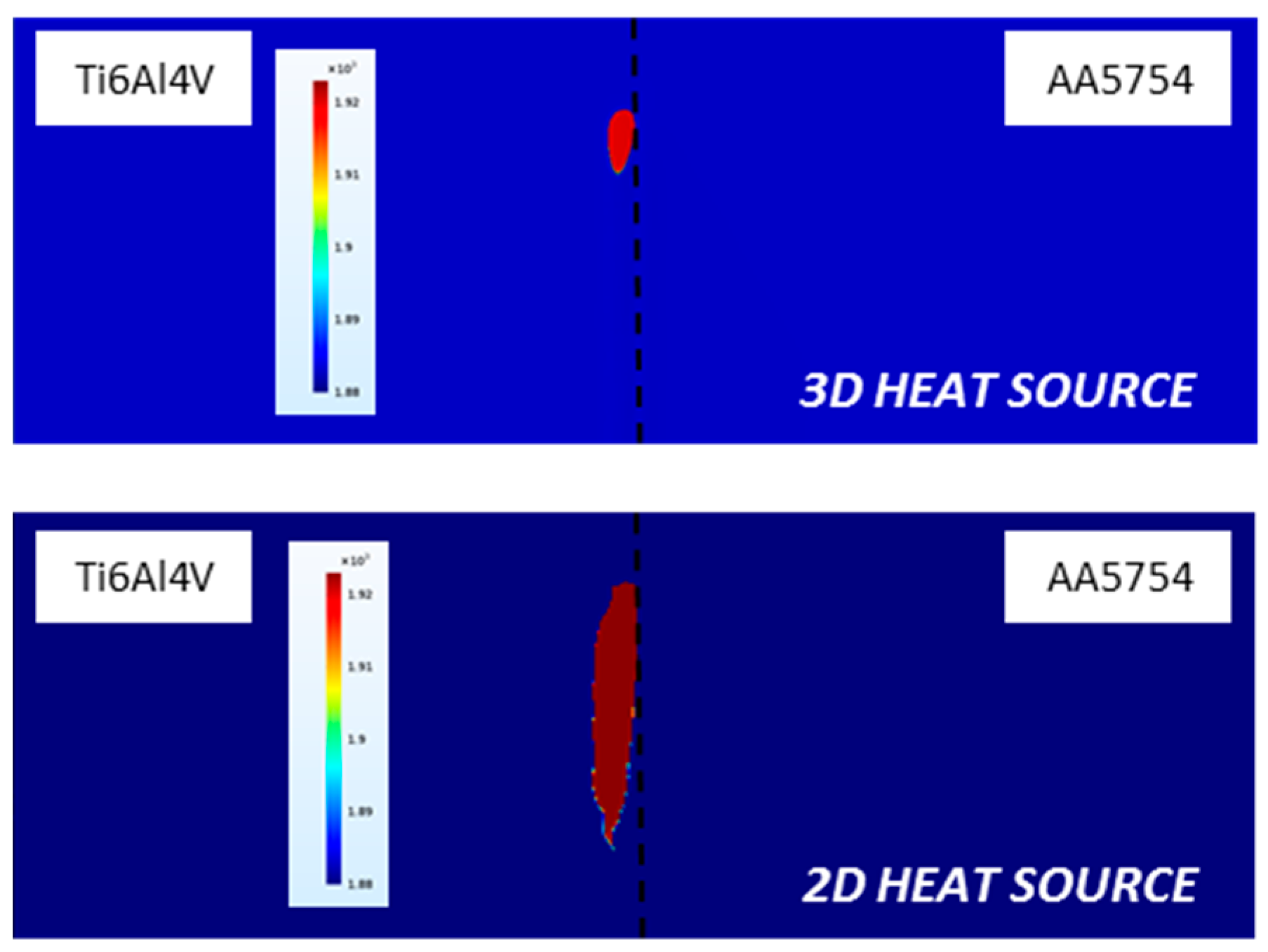
Figure 14.
Interface zoom-up in the weld cross section ns.
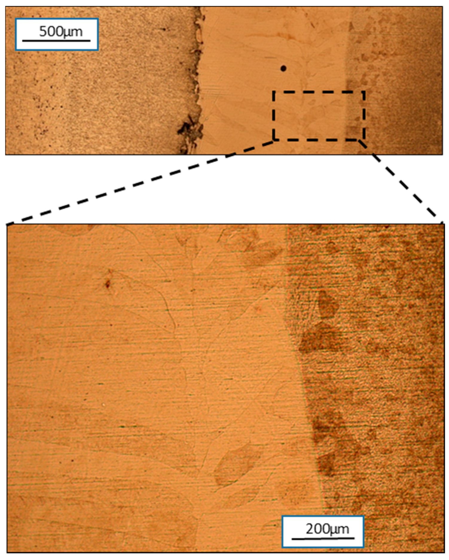
Figure 15.
Experimental and numerical thermal cycle using 2D heat source modelling.
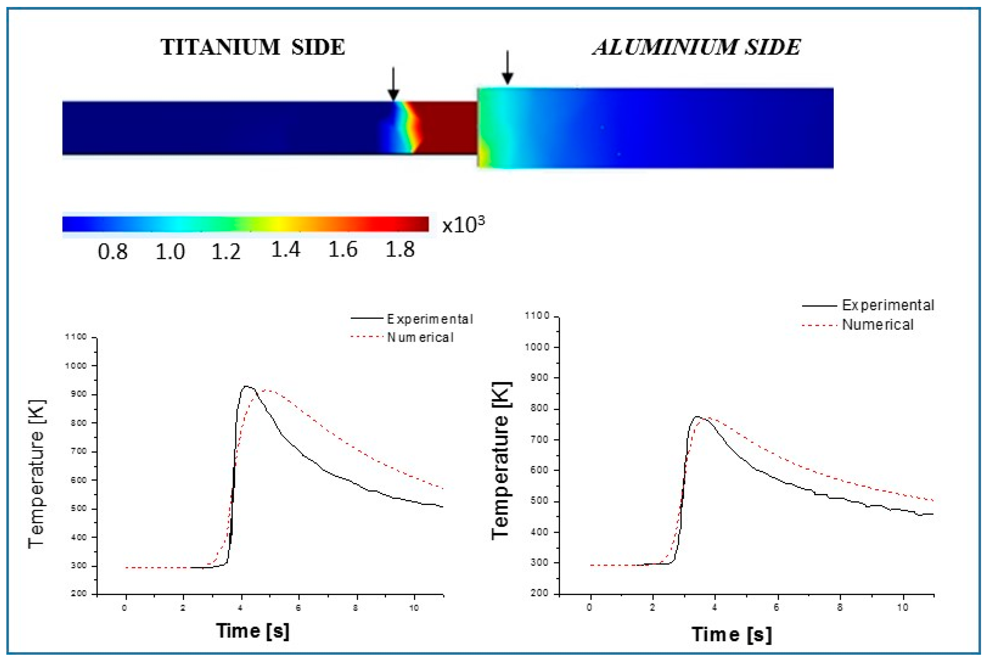
Figure 16.
Experimental and numerical thermal cycle using 3D heat source modelling.


Table 1.
Chemical composition of AA5754 aluminum and Ti6Al4V titanium alloys (wt %).
| AA5754 | ||||||||
| Si | Fe | Cu | Mn | Mg | Cr | Zn | Ti | Al |
| 0.40 | 0.40 | 0.10 | 0.50 | 2.6–3.6 | 0.30 | 0.20 | <0.15 | balance |
| Ti6Al4V | ||||||||
| C | Fe | N2 | O2 | Al | V | H2 | Ti | C |
| <0.08 | <0.25 | <0.05 | <0.2 | 5.5 | 3.5 | <0.0375 | balance | <0.08 |
Table 2.
Mechanical and thermo-physical properties of the two alloys.
| Property | AA5754 | Ti6Al4V |
|---|---|---|
| Young modulus [GPa] | 70 | 114 |
| Poisson ratio | 0.3 | 0.3 |
| Density [g/cm3] | 2.7 | 4.4 |
| Liquidus Temperature [K] | 870 | 1923 |
| Solidus Temperature [K] | 856 | 1880 |
Table 3.
Temperature dependent thermal conductivity of AA5754.
| AA5754 | |
|---|---|
| Temperature | Thermal Conductivity [W/mK] |
| 293 | 138 |
| 373 | 147.2 |
| 473 | 152.7 |
| 573 | 162.7 |
| 673 | 152.7 |
| 773 | 158.75 |
| 873 | 138 |
| 1773 | 138 |
Table 4.
Temperature dependent thermal conductivity of Ti6Al4V.
| Ti6Al4V | |
|---|---|
| Temperature | Thermal Conductivity [W/mK] |
| 293 | 6.01 |
| 773.15 | 14.78 |
| 793.15 | 15 |
| 823.15 | 15.15 |
| 953.15 | 17.20 |
| 993.15 | 17.80 |
| 1013.15 | 18.30 |
| 1053.15 | 18.80 |
| 1093.15 | 19.50 |
| 1113.15 | 20 |
| 1133.15 | 20.50 |
| 1153.15 | 21 |
| 1173.15 | 21.60 |
| 1273.15 | 23.91 |
| 1933.15 | 34.3 |
Table 5.
Dimension (mm) of the fusion zone profile in the aluminum side.
| Aluminum Fusion Zone | 2D Heat Source | 3D Heat Source | Experimental Data |
|---|---|---|---|
| Top | 118 | 136 | 116 |
| Middle | 120 | 135 | 112 |
| Bottom | 114 | 135 | 108 |
Table 6.
Dimension (mm) of the fusion zone profile in the titanium side.
| Titanium Fusion Zone | 2D Heat Source | 3D Heat Source | Experimental Data |
|---|---|---|---|
| Top | 232 | 204 | 225 |
| Middle | 207 | 196 | 198 |
| Bottom | 226 | 187 | 196 |
© 2017 by the authors. Licensee MDPI, Basel, Switzerland. This article is an open access article distributed under the terms and conditions of the Creative Commons Attribution (CC BY) license (http://creativecommons.org/licenses/by/4.0/).
Share and Cite
MDPI and ACS Style
D’Ostuni, S.; Leo, P.; Casalino, G. FEM Simulation of Dissimilar Aluminum Titanium Fiber Laser Welding Using 2D and 3D Gaussian Heat Sources. Metals 2017, 7, 307. https://doi.org/10.3390/met7080307
AMA Style
D’Ostuni S, Leo P, Casalino G. FEM Simulation of Dissimilar Aluminum Titanium Fiber Laser Welding Using 2D and 3D Gaussian Heat Sources. Metals. 2017; 7(8):307. https://doi.org/10.3390/met7080307
Chicago/Turabian StyleD’Ostuni, Sonia, Paola Leo, and Giuseppe Casalino. 2017. "FEM Simulation of Dissimilar Aluminum Titanium Fiber Laser Welding Using 2D and 3D Gaussian Heat Sources" Metals 7, no. 8: 307. https://doi.org/10.3390/met7080307
Note that from the first issue of 2016, this journal uses article numbers instead of page numbers. See further details here.