Electrical Resistivity Measurement of Carbon Anodes Using the Van der Pauw Method
by
Geoffroy Rouget
1,2, 
Hicham Chaouki
2,
Donald Picard
2,
Donald Ziegler
3 and
Houshang Alamdari
1,2,* 1
Department of Mining, Metallurgical and Materials Engineering, Laval University, Quebec, QC G1V0A6, Canada
2
NSERC/Alcoa Industrial Research Chair MACE and Aluminum Research Center, Laval University, Quebec, QC G1V0A6, Canada
3
Alcoa Primary Metals, Alcoa Technical Centre, 859 White Cloud Road, New Kensington, PA 15068, USA
*
Author to whom correspondence should be addressed.
Metals 2017, 7(9), 369; https://doi.org/10.3390/met7090369
Submission received: 27 July 2017
/
Revised: 7 September 2017
/
Accepted: 8 September 2017
/
Published: 13 September 2017
(This article belongs to the Special Issue Selected Papers from the International Committee for Study of Bauxite, Alumina & Aluminium 2016)
Abstract
:The electrical resistivity of carbon anodes is an important parameter in the overall efficiency of the aluminum smelting process. The aim of this work is to explore the Van der Pauw (VdP) method as an alternative technique to the standard method, which is commonly used in the aluminum industry, in order to characterize the electrical resistivity of carbon anodes and to assess the accuracy of the method. For this purpose, a cylindrical core is extracted from the top of the anodes. The electrical resistivity of the core samples is measured according to the ISO 11713 standard method. This method consists of applying a 1 A current along the revolution axis of the sample, and then measuring the voltage drop on its side, along the same direction. Theoretically, this technique appears to be satisfying, but cracks in the sample that are generated either during the anode production or while coring the sample may induce high variations in the measured signal. The VdP method, as presented in 1958 by L.J. Van der Pauw, enables the electrical resistivity of any plain sample with an arbitrary shape and low thickness to be measured, even in the presence of cracks. In this work, measurements were performed using both the standard method and the Van der Pauw method, on both flawless and cracked samples. Results provided by the VdP method appeared to be more reliable and repeatable. Furthermore, numerical simulations using the finite element method (FEM) were performed in order to assess the effect of the presence of cracks and their thicknesses on the accuracy of the VdP method.
1. Introduction
The Hall–Héroult process [1,2] is used to perform the electrolysis of alumina. To this end, an electrical current is applied through the electrolytic bath between carbon anodes and cathodes. The carbon anodes are used to provide carbon for the chemical reaction, as well as the electrical current necessary for the electrolysis. To ensure the proper functioning of the electrolysis cells, carbon anodes are subject to quality controls such as chemical reactivity [3,4] or mechanical properties such as strength [5] or density [6] during their production. The quality control is performed on core samples, and usually extracted from the top of the anodes beside the stub holes. This location may lead to core samples having some structural flaws, especially at their bottom [7,8,9]. Core sampling itself may also induce cracks in the samples [10]. The electrical resistivity characterization of anode cores is achieved using the ISO 11713 standard method. This method is merely an adaptation of ASTM B193-02, which is used as a test method for the resistivity of electrical conductor materials, although this latter method requires a sample with neither cracks nor visible defects. Cracks located in the transverse axis (placed normal to the revolution axis of the sample) may most probably induce overestimated values on the measured electrical resistivity, which would not necessarily be representative of the electrical resistivity of the whole anodic block. To overcome this drawback, the Van der Pauw (VdP) method, developed to measure the electrical resistivity of samples with various shapes, represents a potential solution [11,12]. Koon studied the effect of size and place of contacts using the VdP method [13]. De Vries and Wieck targeted the current distribution in certain shapes of samples [14]. Rietveld et al. investigated the accuracy of the VdP method on several shapes of samples [15]. Kasl C. and Hoch M.J.R. [16] proposed a study using the VdP method on circular and cylindrical samples. This study shows that samples with a thickness smaller than their diameter give an accurate value of electrical resistivity. In addition, as exposed by Kasl and Hoch contacts placed along the edge of the sample are preferred to those placed on the top of the sample. Using the VdP method enables the use of samples much smaller than those used with ISO 11713 Standard. Therefore, by reducing the size of the sample, the risk of the presence of flaws reduces.
In this study, the reliability of the VdP method for the electrical characterization of carbon anodes was investigated and compared with the standard method, which is currently used in the aluminum industry. Finally, defects were intentionally introduced to the anode cores, and their electrical resistivity was measured using both methods in order to assess their sensitivity to the presence of defects.
The first part of this work consists of the comparison of both standard and VdP methods to confirm the reliability of the use of the VdP method for carbon anodes. In the second part, the electrical resistivity of industrial core samples is measured, and the results are compared with the values obtained by the industrial practice. For the third part of this study, another set of experiments is performed on the same batch of anode cores, as used in the preliminary experiment, in order to measure the effect of defect orientation on the measured electrical resistivity. Finally, finite element simulations were performed in order to verify the accuracy of the previously performed experiments, and to validate the use of the VdP method for cracked anode cores.
2. Experimental
For both methods performed in the laboratory, the 1 ampere current is provided by a DC Power Supply GW-INSTEK, GPS-3030D, (GW-INSTEK, Taipei, Taiwan). Current and voltage are measured with an Agilent 34461A 61/2 Digit Multimeter (Agilent Technologies, Santa Clara, CA, USA).
2.1. Standard Method
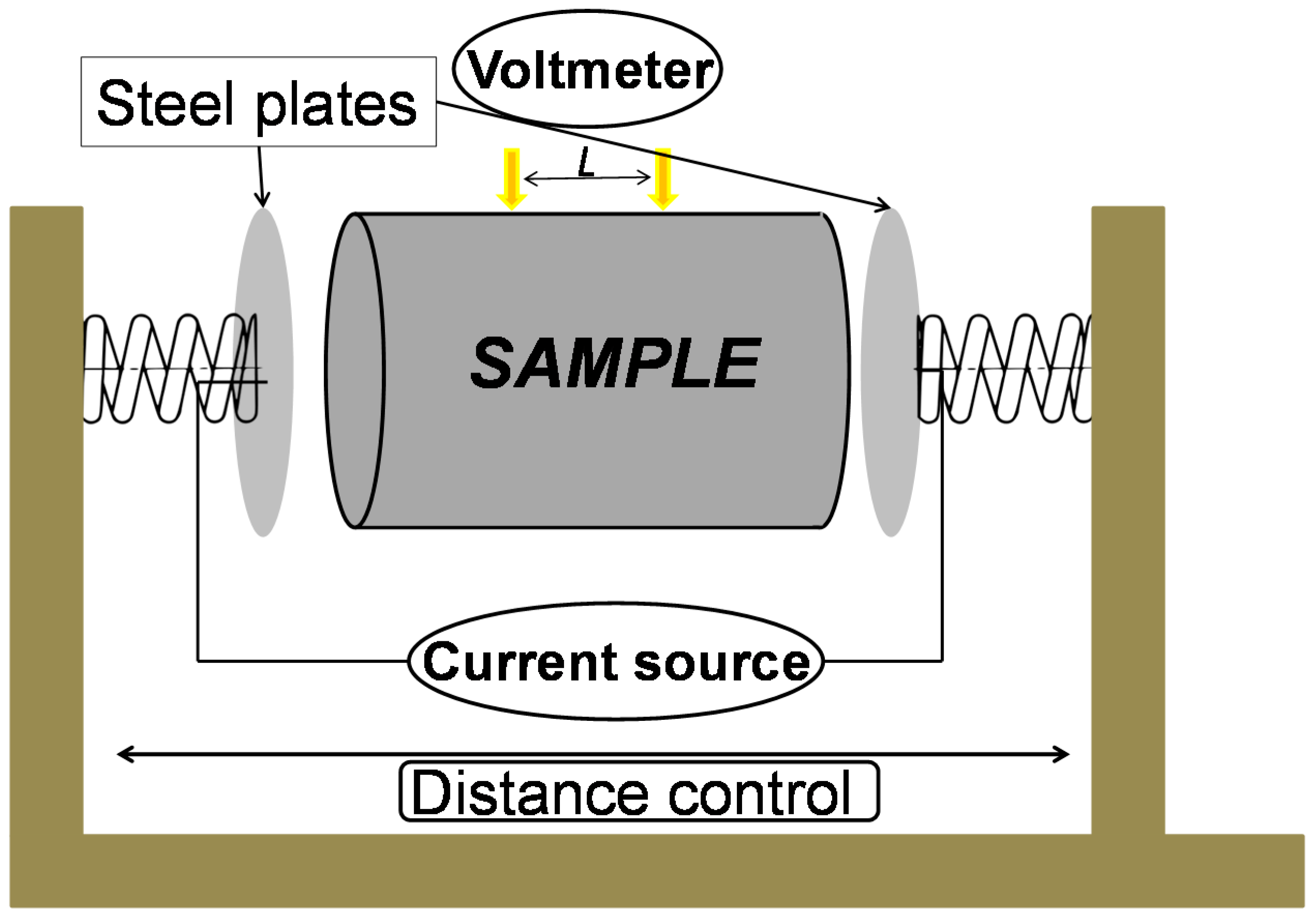
In the case of the standard method, the sample was maintained between two steel plates, both placed on springs to apply 3 MPa pressure, which is required by the standard. Voltage drop was measured with two thin pins mounted on spring, in order to apply the same pressure on each spot. These pins are located on a handle, keeping the same distance apart. The experimental setup is presented schematically in Figure 1. Measurements according to the industrial practice were performed using the R&D Carbon RDC 150 for Specific Electrical Resistance apparatus (R&D Carbon, Sierre, Switzerland).
To calculate the electrical resistivity of anode core using the ISO 11713, the following equation is used:
where ρ is the electrical resistivity of the material, V is the voltage drop measured, I is the intensity of the current applied, S is the cross-section of the sample, and L is the length between the voltage probes, as shown in the Figure 1.
2.2. Van der Pauw Method
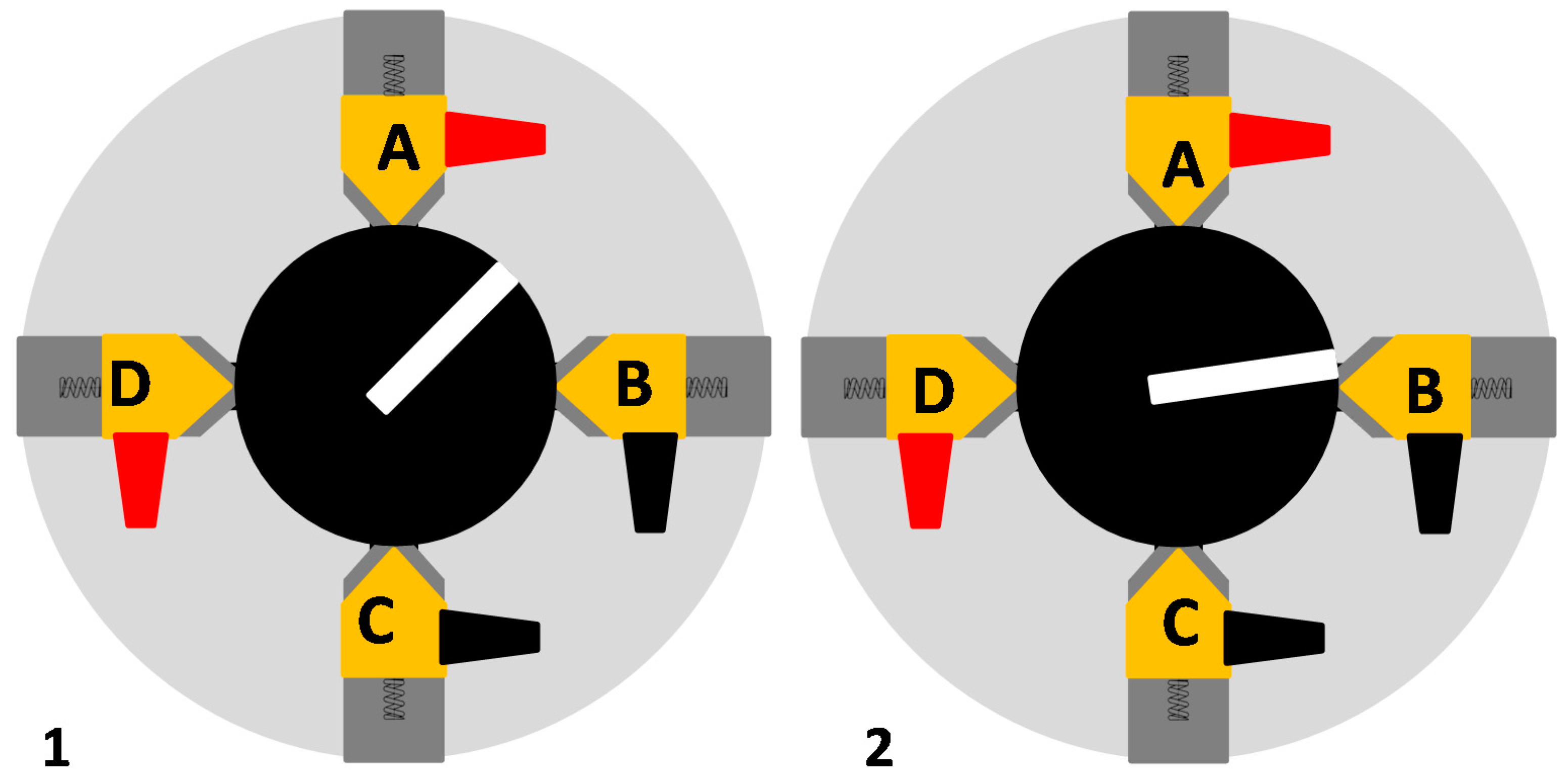
For the Van der Pauw method, since it was decided to take advantage of the cylindrical symmetry, the sample holder was made of a self-centering chuck, which is designed for lathes. Current suppliers and voltage probes were made of copper bars, with a V-shape facing the sample edge, in order to minimize the contact area, as represented in Figure 2.
Each copper bar is mounted with springs on plastic jaws that slide on the chuck’s body (Figure 2). The plastic jaws are used to ensure a good electrical insulation between each copper bar and the chuck. The scroll ring turns to adjust the opening of the probes. All of the probes are related to move at the same time and with the same distance, in order to keep the sample always centered. As presented by Van der Pauw method [11,12], the electrical resistivity, the resistance, and the thickness of the sample between two contiguous sets of points of measurement on its edge must be related by the following equation:
where L is the thickness of the sample (m); RAB,DC is the measured electrical resistance when the current is injected between probes A and B, and the voltage drop is measured between D and C (μΩ); RBC,AD is the resistance measured when the current is injected between probes B and C, and the voltage drop is measured between A and D (μΩ); and ρ is the electrical resistivity (μΩ∙m).
For the standard method performed in the laboratory, four measurements were performed around each sample. The average value and the standard deviation were calculated. For the VdP method, eight measurements were performed: four in a first position, and four after rotating the sample by 45°. Considering the top view of the setting, which is presented in Figure 2 and the Equation (2), it can be seen that a pair of two contiguous measurements are required to obtain a single value of electrical resistivity. Due to this requirement, four values of electrical resistivity would be obtained after the eight measurements. The average electrical resistivity and standard deviation were obtained after the four electrical resistivities were calculated. To avoid positioning errors, the sample remained in the sample holder the entire time for each set of four measurements, and only the wires from the copper bars were changed.
2.3. Samples Preparation
A first series of experiments allowed comparing the ISO 11713 standard method and the VdP method. To this end, eight samples, named 1 to 8, and each with a diameter of 5 cm and a length of 10 cm, were cored from the bottom of a single anode block. The electrical resistivity of each sample was measured using both techniques. This part was done to compare the reproducibility of the measurement, and assumed that the samples would have very close resistivity, as they were taken from the same anode block.
To emphasize the comparison between the two techniques, a second series of experiments was carried out. Six industrial samples were tested, using the VdP method and the ISO 11713 standard method. All of the samples had their electrical resistivity measured previously using routine industrial practice (R&D Carbon method). Three samples were intact (in appearance), named Samples A, B and C, and the three other presented noticeable defects (broken into two pieces), named D, E and F. The intact samples were tested using the standard method at the university laboratory in order to compare the results with those obtained by the industrial laboratory. After the measurement using the standard method, three slices were cut out of the samples between the locations of the voltage probes. The electrical resistivity of each slice was measured using the VdP method. The position of the slices in an anode core is presented in Figure 3.
The three samples containing defects were directly cut in three slices, as their condition would not allow measuring their resistivity using the standard method. Figure 4 shows the condition of the broken anode core after sampling for measurement by the VdP method.
The third and last series of experiments was done in order to identify the effect of noticeable defects in the sample on the measured electrical resistivity. The defects were intentionally created in the sample. Samples were machined to create cracks placed in radial and in transversal positions, as shown in the Figure 5(A-2,B-2). The samples used in this experiment were taken from the same anode as those used for the first set of measurements.
The measurements were performed on samples containing defects before cutting, using the standard method, and then after cutting, using the VdP method. Finally, numerical simulations were carried out to verify the predictive capabilities of the Van der Pauw method. To this end, an electrical model was developed in the Abaqus software [17]. In these simulations, the anode electrical resistivity is prescribed. The electrical resistances of Equation (2) are estimated. Then, the electrical resistivity corresponding to the VdP model is calculated, by solving Equation (2), and comparing it with the prescribed value. Moreover, by considering samples with different crack configurations, it is possible to evaluate the effect of these cracks on the accuracy of the VdP method.
3. Results
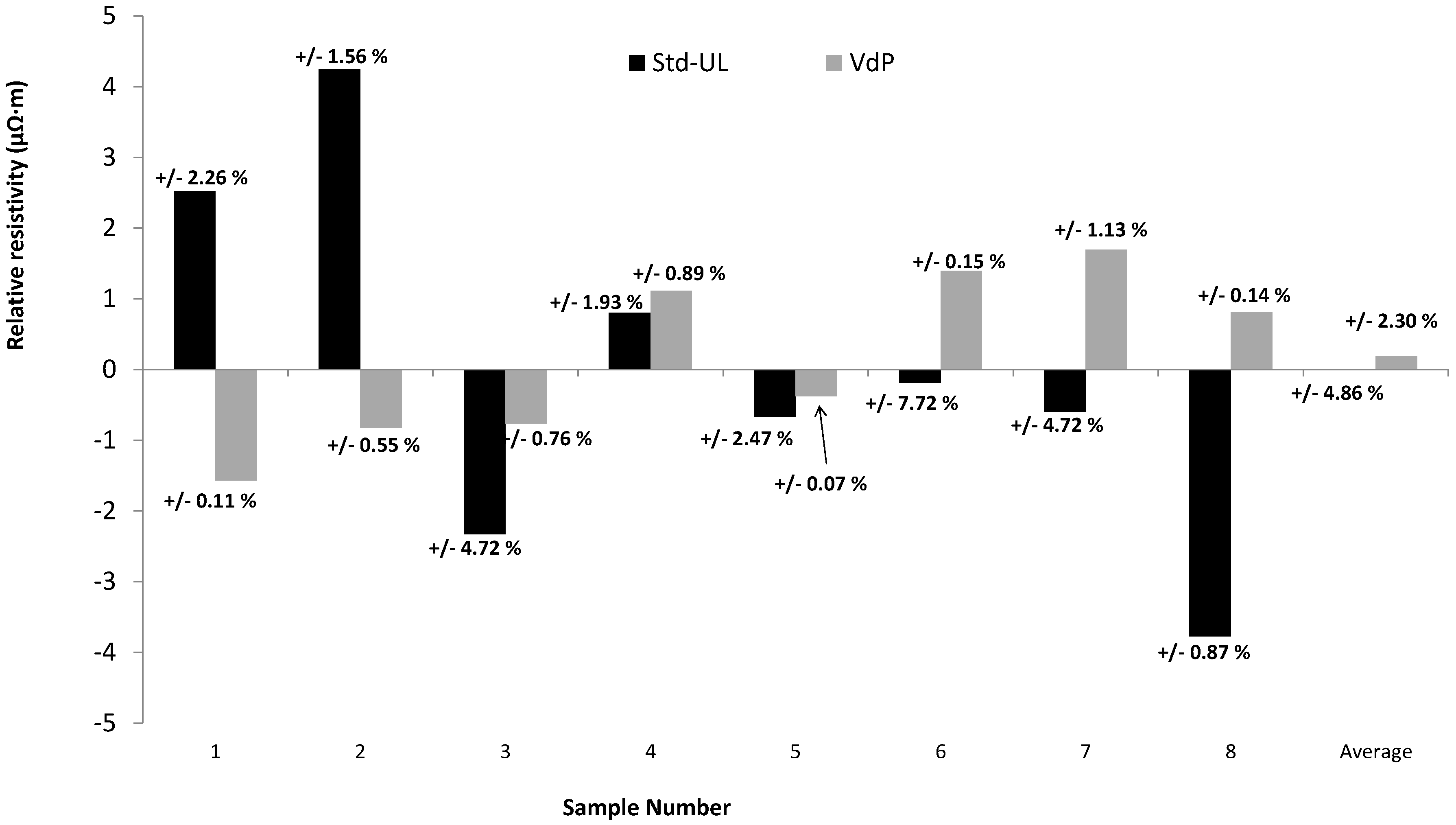
All of the values presented in the experimental part are the resistivity values relative to the average of the measurements performed on the first eight samples using the ISO 11713 standard method, in which the average resistivity measured was of 52.5 μΩ∙m. The results presented are thus a relative electrical resistivity, and a negative value refers to a measured electrical resistivity smaller than the average value obtained via standard method.
3.1. Comparison of Standard and Van de Pauw Methods
The graph presented in Figure 6 shows the values of the relative electrical resistivity of these samples. The baseline of this graph is the average value of eight measurements obtained by the ISO 11713 standard method. The standard deviation of the measurements is presented as percentage of the absolute measured value, and indicated on each value. The data points marked as “average” on the graph represent the average value of all eight measurements performed by two techniques, thus the relative value for the ISO 11713 standard method is zero. The results show that the standard deviations of the VdP method are much smaller than those obtained by the standard method. It can be noted from the ninth set of columns, named “Average”, that the average value obtained using the VdP method is very close to the one obtained using the standard method, while the standard deviation of the former is half that of the standard method. This first set of measurements showed the high accuracy of the VdP method for characterizing the electrical resistivity of the anode core.
3.2. Validation of Van der Pauw Method for Intact Samples
In the second set of measurements, the three intact industrial samples (A, B and C) were tested. All the samples originated from the same anode plant, Plant 1. The results obtained in the industrial laboratory are labeled as “Indus”. Then, those obtained using the four-point measurements of the standard method are labeled as STD-UL. The three slices cut out of each anode core, between the locations of the voltage sensors, in order to use the VdP method were labeled VDP-1, VDP-2 and VDP-3, respectively. Finally, the mean electrical resistivity of each sample was calculated using the VdP method, and labeled as VDP-AVG. The results of the measurements are presented in Figure 7. It can be seen that the electrical resistivity measured at the industrial laboratory and in our laboratory are very close when using the standard method. We notice that standard deviation for tests carried out in the industrial laboratory were not provided.
The samples A, B and C were cored from different anode blocks that were provided by the same anode plant. This means they share the same raw materials and anode-forming process. However, they show a strong difference in electrical resistivity measured by the standard method, both at the industrial laboratory and at the university (Indus and STD-UL respectively). On the other hand, the results obtained through the VdP method show that the electrical resistivity values for the three samples are very close to each other. In addition, the standard deviations were smaller compared with those provided by the standard method, which suggested that the VdP method could be a more accurate technique of measurement. The drastic change in results measured using the standard method, both by the industrial partner and at the university, and the VdP method can be explained. When the standard method is used, the current flows through the sample along the axis of revolution (Figure 5(A-1)), but the voltage drop is measured only on the edge of the sample. During the core sampling of the anode, microcracks and coarse particles containing their own defects can be produced, which may strongly influence the current flow at the specific area of measurement. However, these defects probably cannot be seen with the naked eye. On the other hand, when using the VdP method, the current flows normally to the axis of revolution (Figure 5(B-1,B-2)), parallel to the cross-section of the sample. This implies that the defects generated during the machining on any of the edges of the sample, may not have a strong influence on the measurements performed. It is suggested by the author that the measurement using the standard method occurs at the surface, while when using the VdP method, the measurement is over the volume.
3.3. Validation of Van der Pauw Method for Broken Samples
Another set of tests was performed on three samples provided by the industrial partner, and containing noticeable flaws, as shown in Figure 4. Samples D and E originated from the same anode plant (Plant 2), while sample F came from a different anode plant (Plant 3). These samples were already broken upon reception. This condition prevented the performance of any measurement using the standard method. In this case, only the measurements provided by the industrial partner (standard) and VdP methods are compared. The anode core pieces were long enough to cut three slices out of each sample. Figure 8 presents the results provided by the industrial laboratory and those obtained using the VdP method. Similar to the previous set of samples, the industrial laboratory did not provide the standard deviation for the measurements.
It can be seen that there are strong differences between samples D and E when the standard method was used in the industrial laboratory. However, the VdP method showed that they exhibit very close relative electrical resistivities (−4.57 μΩ∙m for D and −4.91 μΩ∙m for E). The two samples D and E showed a similar electrical resistivity using the VdP method, which might be because the same raw materials and anode-forming process were used in the anode plant. For sample F, the standard and VdP methods lead to the same results.
3.4. Validation of Van der Pauw Method for Intentionally-Generated Cracked Samples
Finally, measurements were conducted on the samples containing noticeable intentionally-generated cracks. For all of the following experiments, the samples for the VdP method were sliced to 1 cm thick and 5 cm in diameter. To simplify the problem, cracks were made either along the revolution axis (radial crack), or normal to it (transverse crack).
A radial crack was generated on a sample before slicing. This allowed performing electrical measurements by the standard method, both before and after performing the slice cut. Then, three slices were cut out of the sample to measure the electrical resistivity using the VdP method. In such a situation, two positions were used for the crack toward the probes. In one position, the crack was placed at an equal distance between two probes. In the other position, the crack was placed close to one of the probes (Figure 9). Those options were chosen to assess the effect of position of the crack on the results.
The tests were also performed on samples that had transversal cracks (normal to the revolution axis). In order to compare the standard and VdP methods, cracks were created before slicing. A side view of the cracked sample is shown on Figure 5(B-2). The obtained results were summarized in Table 1. As the surface and length of samples were taken into account for the electrical resistivity calculation using the standard method, the void corresponding to the crack generation had to be removed from the total sample volume. We recall that the presented values are related to the average value of the electrical resistivity measured in the first experiments, while the standard deviation is related to the real obtained values.
The results presented in Table 1 clearly show that when using the standard method, a noticeable difference is measured between the sample without any cracks, and the sample containing a crack. The electrical resistivity is overestimated in the presence of cracks. Moreover, it seems that the crack orientation substantially affects the measurements provided by the standard method. The results obtained using the VdP method show that this technique is considerably less sensitive to the cracks’ size and orientation than the standard method. In fact, small differences between relative electrical resistivity measurements for different samples were obtained with the VdP method. The bigger standard deviation is obtained for the transverse crack. The thickness of the crack behaves as a layer of insulating material parallel to the sample itself. Using the VdP technique enables the electrical resistivity to be retrieved when the crack is radial, as it does not interfere with any parameter of calculation. When the crack is placed transversally, it has an influence on the thickness of the sample (parameter “d” in the Equation (2)). This causes an overestimation of the electrical resistivity.
4. Finite Element Modelling of VdP Method
In order to assess the robustness of the VdP method, numerical simulations were carried out using the commercial finite element software Abaqus [17]. The purpose of these numerical simulations was to simulate the experimental set up developed for the VdP method (Figure 2 and Figure 9). Therefore, for a given sample, with or without crack, and an assigned electrical resistivity, all electrical potentials and resistances needed for the VdP method were evaluated numerically. This enabled the estimation of the electrical resistivity of a sample through the VdP method. To this end, the Newton–Raphson scheme for nonlinear equations was used to solve Equation (2). Furthermore, using this approach, some specific cases, such as very thin cracks, which are not easily achievable in laboratory, can be simulated.
In order to reproduce conditions used in the laboratory, a cylindrical sample with 1 cm thickness and a 5 cm diameter was considered. An electrical current of 1 ampere was applied on the supply connector bars. The electrical resistivity of an anode is usually around 50 μΩ∙m (a conductivity of 20,000 S/m) [18]. Figure 10 and Figure 11 show the developed CAD (Computer-Aaided Design) model, and the mesh used for the simulations in the cases of the radial crack placed between two probes (Figure 10A and Figure 11A), and the transverse crack (Figure 11A,B).
Since Abaqus software requires an electrical conductivity as the input, we decided to use the value of 20,000 S/m for simulations. Using the parameters mentioned above, tests were run with each crack configuration presented previously. The electrical potential at the voltage probes was calculated and used in the VdP equation in order to estimate the sample electrical resistivity. For radial and transversal defects, the crack was designed as 2 mm thick and 1.7 cm deep. In the case of the radial crack, simulations were performed with cracks placed between the probes and close to one of the probes, similar to that in the experimental measurements.
A first simulation was run on a simple circular sample. This simulation allowed us to retrieve an electrical resistivity of 49.8 μΩ∙m using the VdP method. This result shows that the error between the assigned electrical resistivity and the calculated one (using the VdP Method) is very small. After the validity of the model was confirmed, tests were run on other configurations. The obtained results are stored in Table 2 and Table 3.
Table 2 shows the simulation results for samples containing a crack parallel to the axis of rotation (Figure 5(A-2)). The crack was placed as follow: (i) between two sensors at equal distance, and (ii) close to one of the sensors. It is expected that, for a defect parallel to the axis of revolution being normal to the electric current line, the volume of the crack does not substantially affect the results. This assumption can be explained in that the VdP equation, Equation (2), is not related to the surface area of the sample, but rather only to its height. Figure 5(A-2) depicts the position of the crack, which in the case of this orientation, does not interfere in the calculation. To justify the latter statement, a simulation was performed on a sample containing an infinitesimally thin crack (0.1 mm), which does not represent any noticeable variation in the volume of the sample. It is important to note that such a thin crack may not be visible to the naked eye. The crack was placed in the same direction, close to one of the sensors. It appears that the obtained results seem to remain stable whether the crack is placed close to a probe, or centered between two, or even if its size is highly reduced. Furthermore, the relative error between the assigned electrical conductivity and the one retrieved using the finite element method (FEM) and VdP methods remains very low.
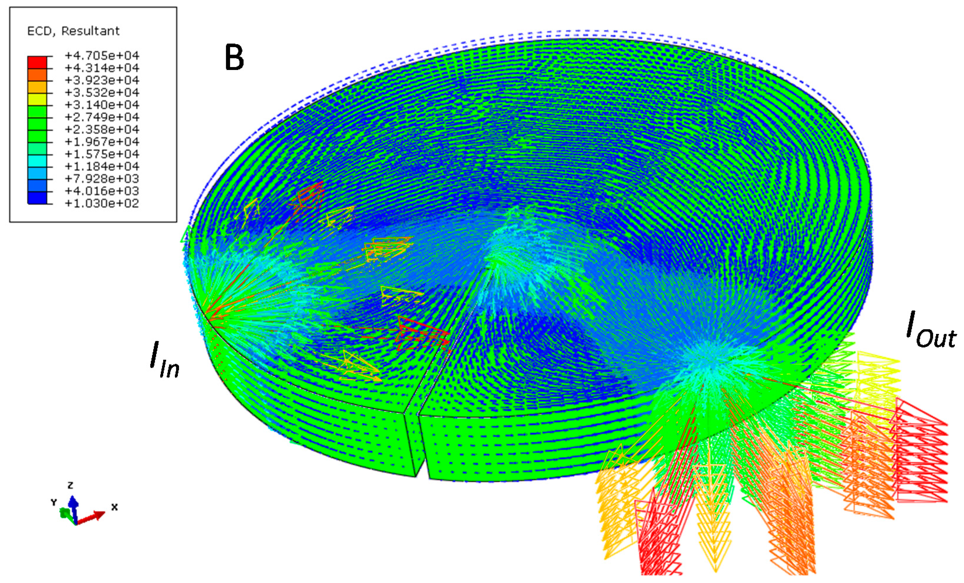
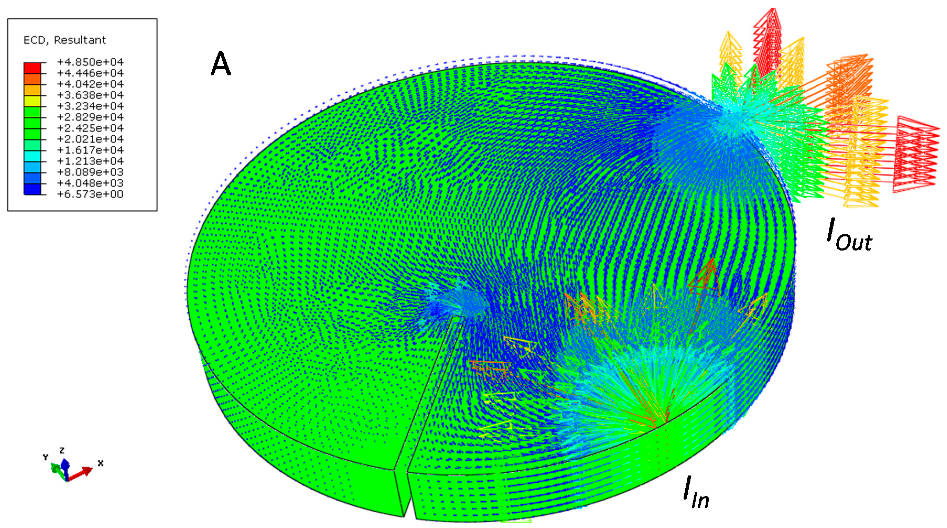
In a second approach, the crack was placed on a plane normal to the axis of rotation (Figure 5(B-2)). In this case, the void interferes with the real height of the sample and most probably affects the results. To justify this assumption, two cases were investigated using the FEM and VdP methods. The crack was initially 2 mm wide in a 10 mm thick sample, which created a non-negligible void within the material. Referring to Figure 5(B-2) and Equation (2), one can easily state that the void created by this crack would most probably affect the calculation of electrical resistivity. After the 2 mm crack, a 0.1 mm crack was placed in the same spot to compare the results. Table 3 shows the results of both simulations. As expected by the authors, the error obtained when the crack is macroscopic is bigger than when the crack in infinitesimally thin. In the case of the thin crack placed normal to the axis of revolution, the error calculated tended to be even smaller than that in the case of the thin crack placed parallel to the same axis. The results presented after both simulations corroborate the hypothesis initially made by the authors; i.e., when the crack is placed normal to the axis of revolution, namely parallel to the current lines, the thickness of the crack will have an influence on the measured electrical resistivity. Moreover, the thickness of the crack will induce a non-negligible volume of void with a higher electrical resistivity, after taking into account the calculation of the electrical resistivity of the sample. This leads to an increase in the calculated electrical resistivity or, as seen in Table 3, a decrease in electrical conductivity. The bigger the crack, the stronger the error will be observed. Figure 12 shows the current lines flowing through the sample in the case of the radial crack. Figure 12A represents the current flowing when the current probes are placed on the same side of the crack; meanwhile, Figure 12B shows the current lines when the current probes are placed on both sides of the crack. In both cases, it can be noticed that the electrical current flows in a plan perpendicular to the revolution axis. These results are in agreement with authors’ hypothesis about the electrical current flow.
5. Detection of Defects Using VdP Method
In the previous section, it was shown that the electrical resistivity could be easily retrieved using the VdP method, even if the sample contains structural flaws. Referring to Equation (2), the VdP method requires the measurement of two contiguous resistances, RAB,DC and RBC,AD, in order to calculate the electrical resistivity of the material. The samples have a cylindrical geometry, and are supposed to be homogeneous in composition. In a crack-free sample, the resistances RAB,DC and RBC,AD present very close values. In the case of samples containing cracks along the axis of revolution, the cylindrical symmetry is lost, and only the axis of symmetry remains along the crack. Thus, the resistances RAB,DC and RBC,AD show a significant difference. In the case of cracks normal to the axis of revolution, such a difference between RAB,DC and RBC,AD is not observed. This can be explained by the orientation of the crack toward the current flow. According to the geometry of the system, one can state that the current flows mostly parallel to the faces of the sample; as a result, defects oriented in the same direction as the current flows will have a lower effect than those placed in a different direction. For simplicity, RAB,DC and RBC,AD are respectively expressed as R1 and R2, hereafter. Table 4 shows the results obtained after the simulations. It reveals that for a crack placed in a radial direction, parallel to the axis of revolution, a strong difference between the two contiguous resistances can be observed, regardless of the thickness or the position of the crack toward the sensors.
On the other hand, Table 5 presents the results obtained in the case of a crack placed normally to the axis of revolution of the sample. This means that the crack shares the direction of the electrical current lines. In this case, referring to Equation (2) and considering the Figure 5(B-2), the parameter “d” is obtained by subtracting the thickness of the crack from the thickness of the sample. Therefore, the thickness of the crack implicitly influences the measured values when the thickness of the crack is not negligible compared with that of the sample. In this configuration, the effect is limited to a diminution of the actual volume of matter through which the current flows. Results presented in Table 5 show that the difference between contiguous probes is very low when compared with the case of a crack normal to the electrical field lines. The difference between the results in the two sections of Table 5 is probably because when a crack is of a non-negligible size, the lack of material to conduct the current, which acts as a much more resistive part, will lead to higher resistance values and therefore a lower electrical conductivity. Consequently, the resistances measured for a 2 mm thick crack are slightly higher than that measured for a 0.1 mm thin crack. Those results are in a good adequacy with the above-mentioned hypothesis.
The difference of values between R1 and R2 can indicate very precisely the presence of cracks, specifically if they are placed parallel to the axis of revolution. According to the obtained results, it seems that the Van der Pauw method, when coupled with FEM, helps detect the presence of defects in an anode core. Depending on the type, size, and orientation of the defects, the detection can be either good or totally inadequate. This method is complementary to the standard method that is usually used for the characterization of the anode core, and could provide better defect detection.
6. Conclusions
In this work, the electrical resistivity of baked carbon anodes used in the aluminum industry was studied using both the ISO 11713 standard method and the Van der Pauw method. Comparison side by side was achieved by experimental analysis; then, numerical simulation was used to emphasize the previously obtained results.
The results obtained experimentally show that on industrially produced anode cores, the Van der Pauw method appears to be more accurate and less sensitive to macro and micro structural defects in the material. As the cracks in anode cores are not necessarily representative of the microstructure of the whole anode, the knowledge of the electrical resistivity of the material without the effect of crack, which can be considered as intrinsic electrical resistivity of the material, gives better information on the electrical properties of the anode block, i.e., inhomogeneity, paste formulation effect, etc. This method shows a good repeatability in the measurement of the electrical resistivity of samples. Numerical simulations using the finite element method showed that this method is perfectly suitable for the measurement of the electrical resistivity of samples containing defects or flaws such as macroscopic cracks, in different orientations. It has to be noted that depending on the size and orientation of the defect toward the sensors, the defect may induce an error in the calculation of electrical resistivity. Also, the Van der Pauw method, complementary with the standard methods ISO 11713, can reveal the presence of defects in the material that cannot be seen by the naked eye. The Van der Pauw method is very simple and easy to use, and would be easy to automate for industrial purposes.
Acknowledgments
The authors gratefully acknowledge the financial support provided by Alcoa Inc., the Natural Sciences and Engineering Research Council of Canada, and the Centre Québécois de Recherche et de Développement de l’Aluminium. A part of the research presented in this article was financed by the Fonds de recherche du Québec-Nature et Technologies by the intermediary of the Aluminium Research Centre–REGAL.
Author Contributions
Geoffroy Rouget and Houshang Alamdari conceived and designed the experiments; Geoffroy Rouget and Hicham Chaouki performed the experiments and numerical simulations; Donald Picard and Donald Ziegler contributed in data analysis; Geoffroy Rouget wrote the paper and all co-authors commented/corrected it.
Conflicts of Interest
The authors declare no conflict of interest.
References
- Hall, C.M. Process of Reducing Aluminium from jts Fluoride Salts by Electrolysis. U.S. Patent 400,664, 2 April 1889. [Google Scholar]
- Héroult, P.L.T. Pour un Procede Electrolytique Pour la Preparation de L’aluminium: An Electrolytic Process for the Preparation of Aluminium bu Paul LT Heroult. French Patent 175,711, 1 September 1886. [Google Scholar]
- Chevarin, F.; Lemieux, L.; Ziegler, D.; Fafard, M.; Alamdari, H. Air and CO2 reactivity of carbon anodes and its constituents: An attempt to understand Dusting phenomenon. Light Met. 2015, 1147–1152. [Google Scholar] [CrossRef]
- Sadler, B.A.; Algie, S.H. Sub-Surface Carboxy Reactivity Testing of Anode Carbon; TMS: San Diego, CA, USA, 1991. [Google Scholar]
- Thibodeau, S.; Chaouki, H.; Alamdari, H.; Ziegler, D.; Fafard, M. Hight temperature compression test to determine the anode paste mechanical properties. Light Met. 2014, 1129–1134. [Google Scholar] [CrossRef]
- Clery, P. Green paste density as an indicator of mixing efficiency. In Proceedings of the TMS Annual Meeting, San Antonio, TX, USA, 15–19 February 1998; pp. 625–626. [Google Scholar]
- Picard, D.; Lauzon-Gauthier, J.; Duchesne, C.; Alamdari, H.; Fafard, M.; Ziegler, D. Automated crack detection method applied to CT images of backed carbon anode. Light Met. 2014, 1275–1280. [Google Scholar] [CrossRef]
- Picard, D.; Alamdari, H.; Ziegler, D.; St-Arnaud, P.-O.; Fafard, M. Characterization of a full-scale prebaked anode using X-ray computerized tomography. Light Met. 2011, 973–978. [Google Scholar] [CrossRef]
- Azari, K.; Alamdari, H.; Aryanpour, G.; Picard, D.; Fafard, M.; Adams, A. Mixing variables for prebaked anodes used in aluminium production. Powder Technol. 2013, 235, 341–348. [Google Scholar] [CrossRef]
- Picard, D.; Alamdari, H.; Ziegler, D.; Dumas, B.; Fafard, M. Characterization of pre-baked anode samples using X-ray computed tomography and porosity estimation. Light Met. 2012, 1283–1288. [Google Scholar] [CrossRef]
- Van der Pauw, L.J. A method of measuring specific resistivity and Hall effect of discs of arbitrary shape. Philips Res. Rep. 1958, 13, 1–9. [Google Scholar]
- Van der Pauw, L.J. A method of measuring the resistivity and Hall coefficient on lamellae of arbitrary shape. Philips Tech. Rev. 1958, 20, 220–224. [Google Scholar]
- Koon, D.W. Effect of contact size and placement, and of resistive inhomogeneities on van der Pauw measurements. Rev. Sci. Instrum. 1989, 60, 271–274. [Google Scholar] [CrossRef]
- De Vries, D.K.; Wieck, A.D. Potential distribution in the van der Pauw technique. Am. J. Phys. 1995, 63, 1074–1078. [Google Scholar] [CrossRef]
- Rietveld, G.; Koijmans, C.V.; Henderson, L.C.A.; Hall, M.J.; Harmon, S.; Warnecke, P.; Schumacher, B. DC Conductivity Measurements in the Van Der Pauw Geometry. IEEE Trans. Instrum. Meas. 2003, 52, 449–453. [Google Scholar] [CrossRef]
- Kasl, C.; Hoch, M.J.R. Effect of sample thickness on the van der Pauw technique for resistivity measurements. Rev. Sci. Instrum. 2005, 76, 033907. [Google Scholar] [CrossRef]
- Abaqus Analysis User’s Guide; Version 6; Dassault Systèmes Simulia Corp.: Providence, RI, USA, 2014.
- Mannweiler, U.; Keller, F. The design of a new anode technology for the aluminium industry. J. Miner. Met. Mater. Soc. 1994, 48, 15–21. [Google Scholar] [CrossRef]
Figure 1.
Schematic view of the setting used for the measurement of electrical resistivity of carbon anodes according to the ISO 11713 standard.
Figure 1.
Schematic view of the setting used for the measurement of electrical resistivity of carbon anodes according to the ISO 11713 standard.

Figure 2.
Picture of the Van der Pauw setting for laboratory measurement. The sample is placed at the center, between the four V-shaped copper probes.
Figure 2.
Picture of the Van der Pauw setting for laboratory measurement. The sample is placed at the center, between the four V-shaped copper probes.
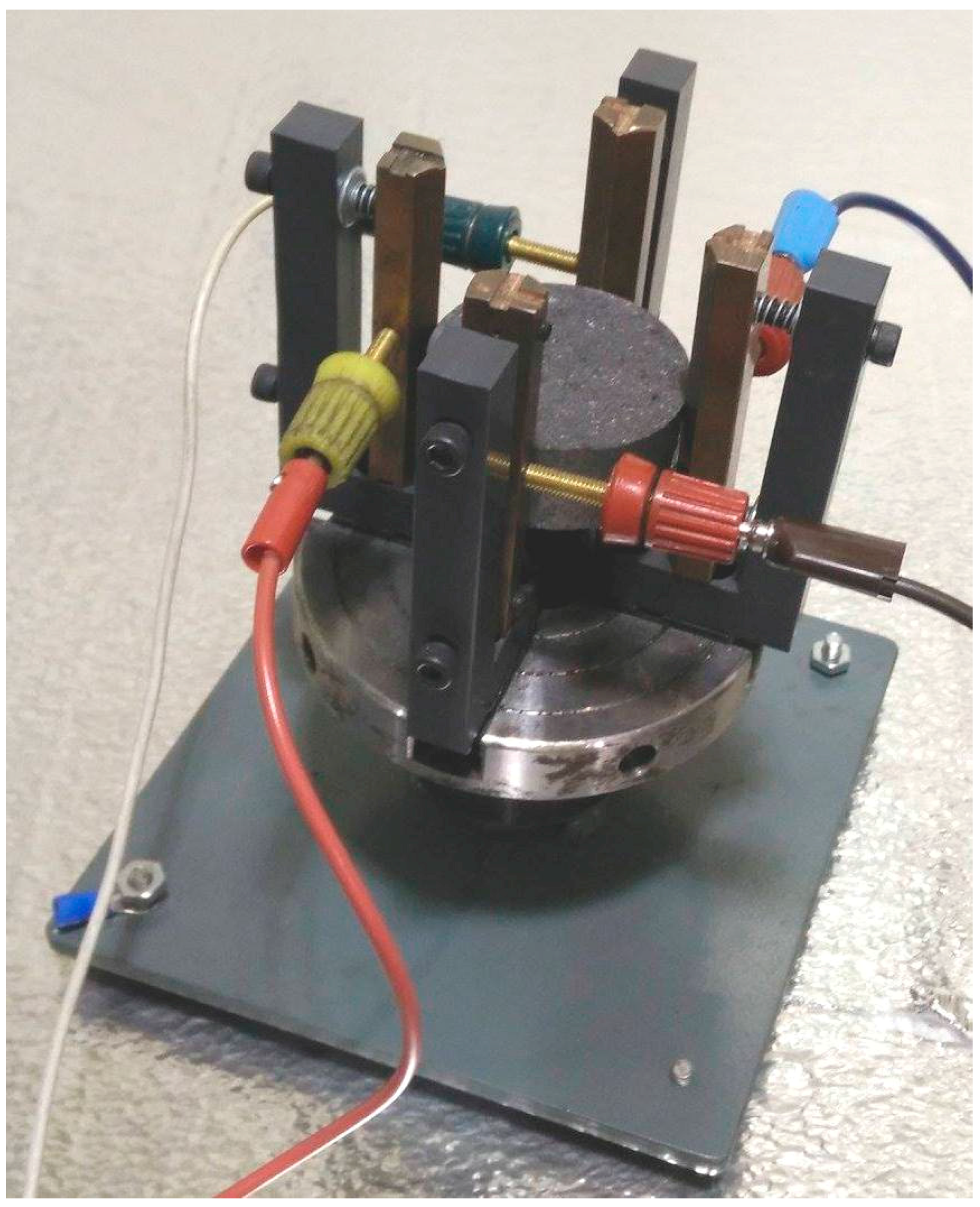
Figure 3.
Anode core shapes for measuring electrical resistivity using the standard method (A) and the Van der Pauw method (B).
Figure 3.
Anode core shapes for measuring electrical resistivity using the standard method (A) and the Van der Pauw method (B).

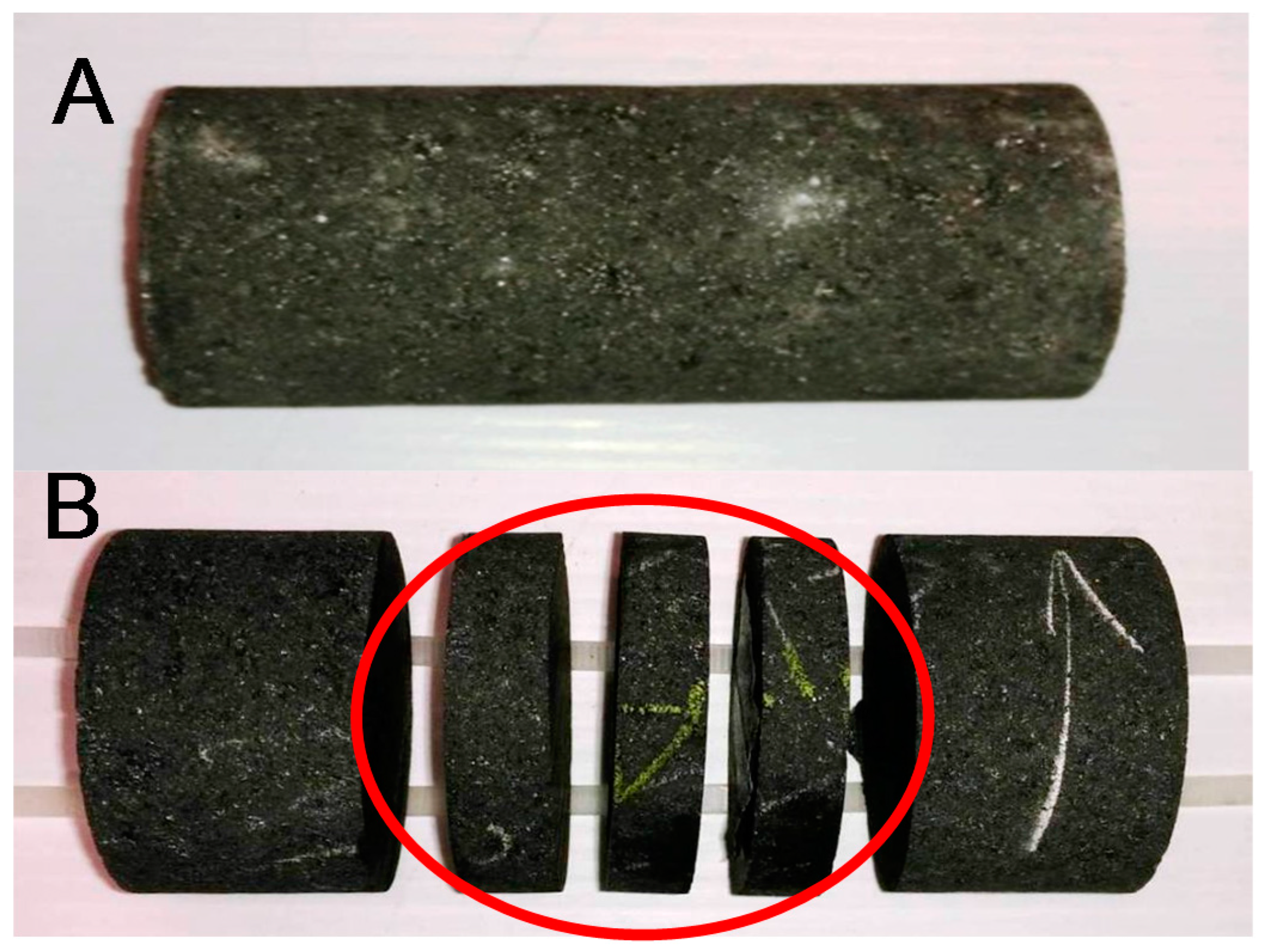
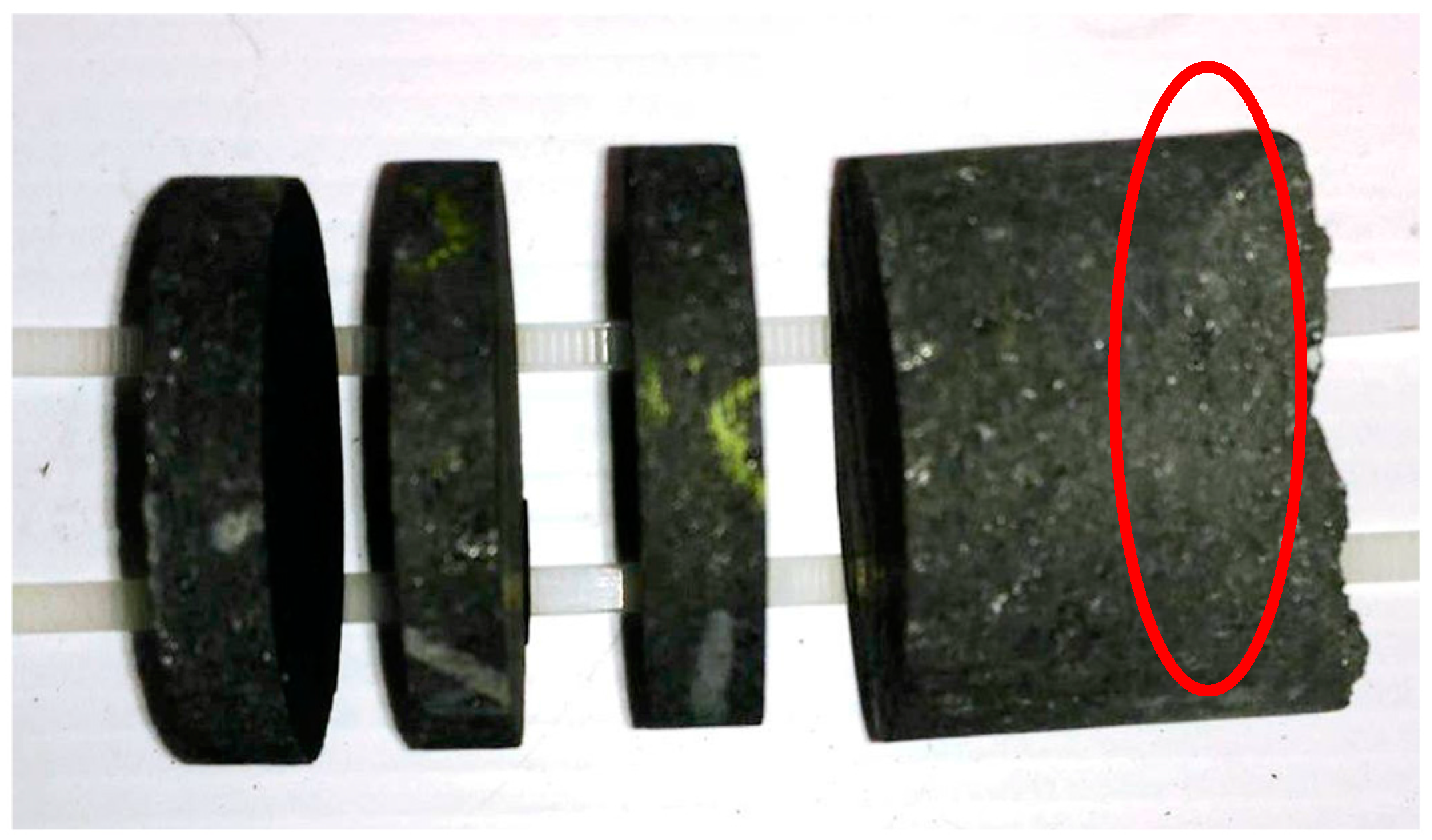
Figure 4.
Broken sample prepared for measurement using the Van der Pauw method. The failure was circled at the right of the sample.
Figure 4.
Broken sample prepared for measurement using the Van der Pauw method. The failure was circled at the right of the sample.

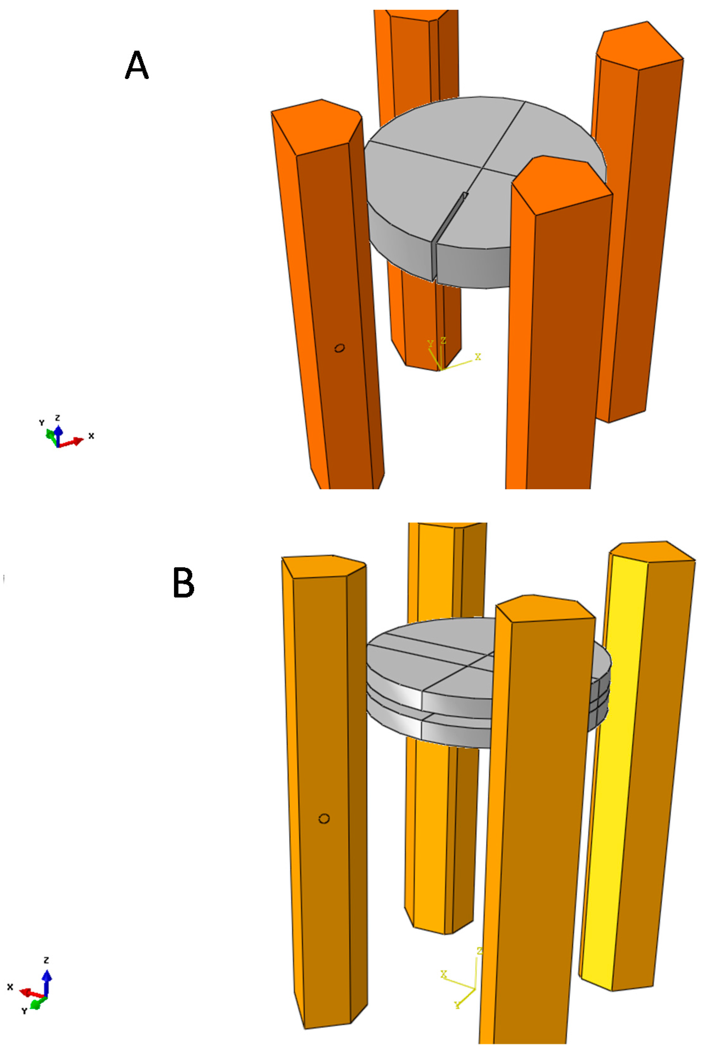
Figure 5.
Schematic view of the cuts performed on sliced samples, along the revolution axis (z-axis) (A-1,A-2) and normal to the revolution axis (B-1,B-2).
Figure 5.
Schematic view of the cuts performed on sliced samples, along the revolution axis (z-axis) (A-1,A-2) and normal to the revolution axis (B-1,B-2).
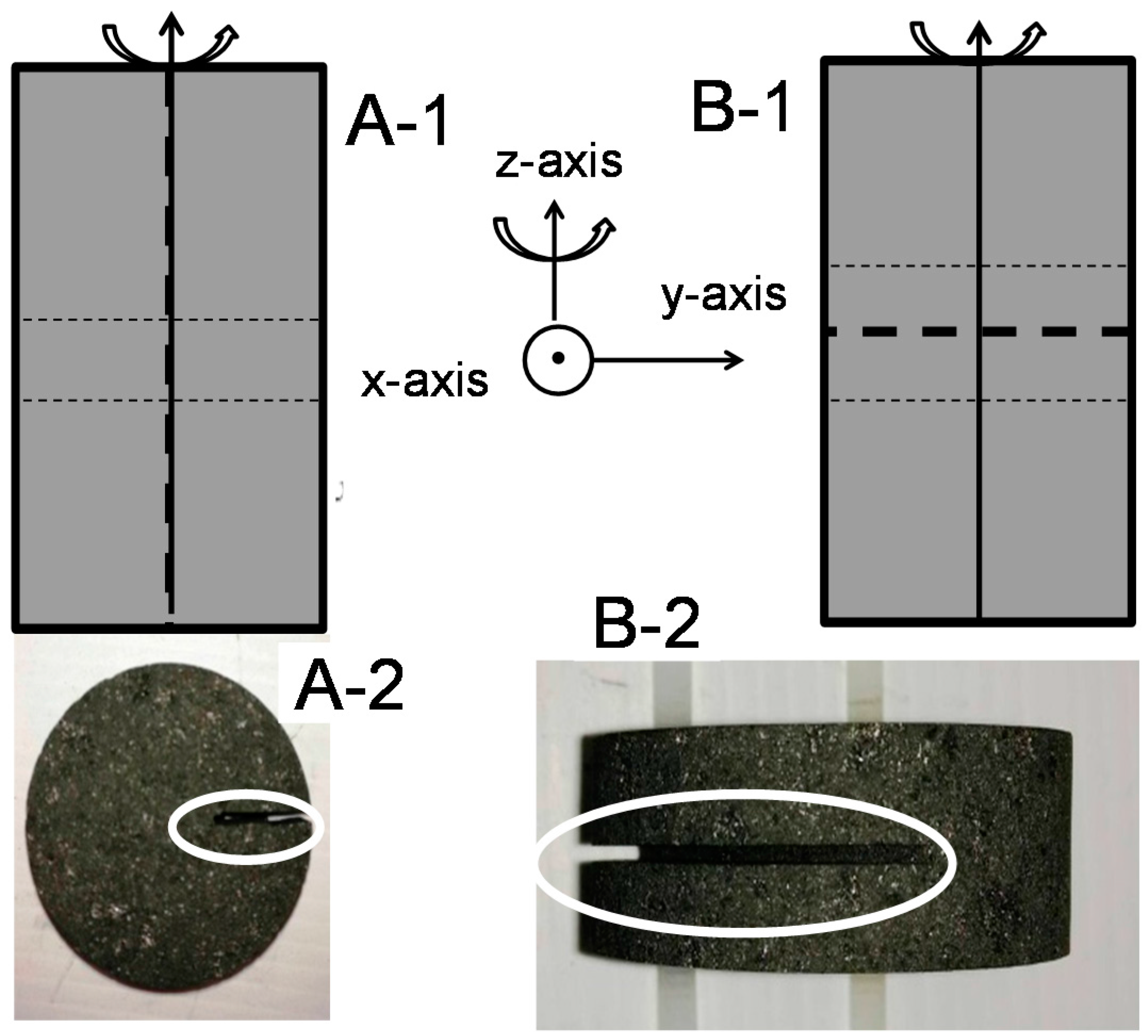
Figure 6.
Comparison of electrical resistivity using the standard and Van der Pauw methods for carbon anode cores.
Figure 6.
Comparison of electrical resistivity using the standard and Van der Pauw methods for carbon anode cores.

Figure 7.
Comparison of standard and Van der Pauw (VdP) methods for intact samples cored from the industrial laboratory. “Indus” and “STD-UL” are the measurements provided respectively by the industrial laboratory and those achieved using standard method in our laboratory. “VDP (1-3)” are measurements performed on slices 1, 2 and 3 of each sample (VdP method); VDP-AVG is the average of the three combined measurements.
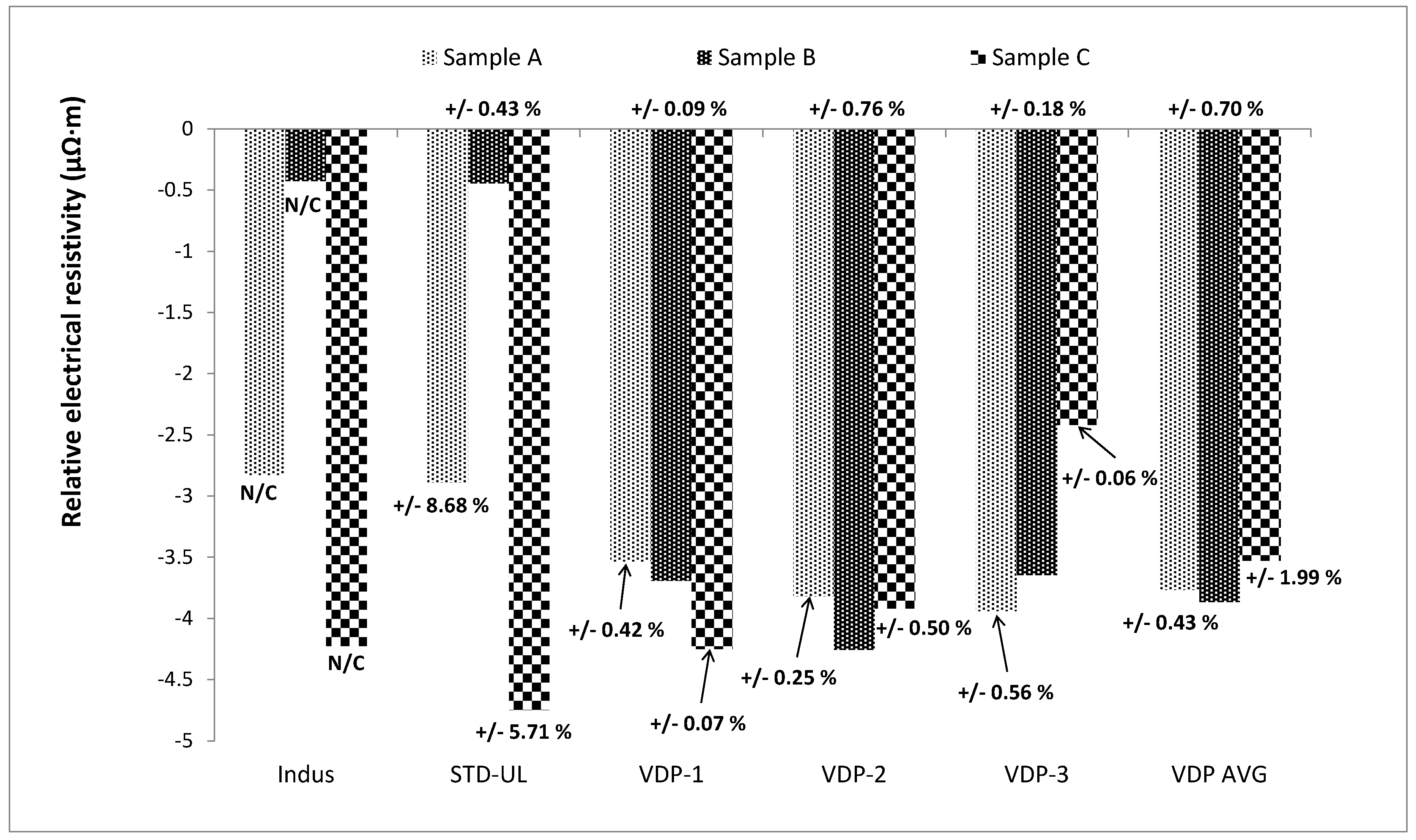
Figure 8.
Comparison of the standard and Van der Pauw methods for flawed samples from the industrial laboratory.
Figure 8.
Comparison of the standard and Van der Pauw methods for flawed samples from the industrial laboratory.
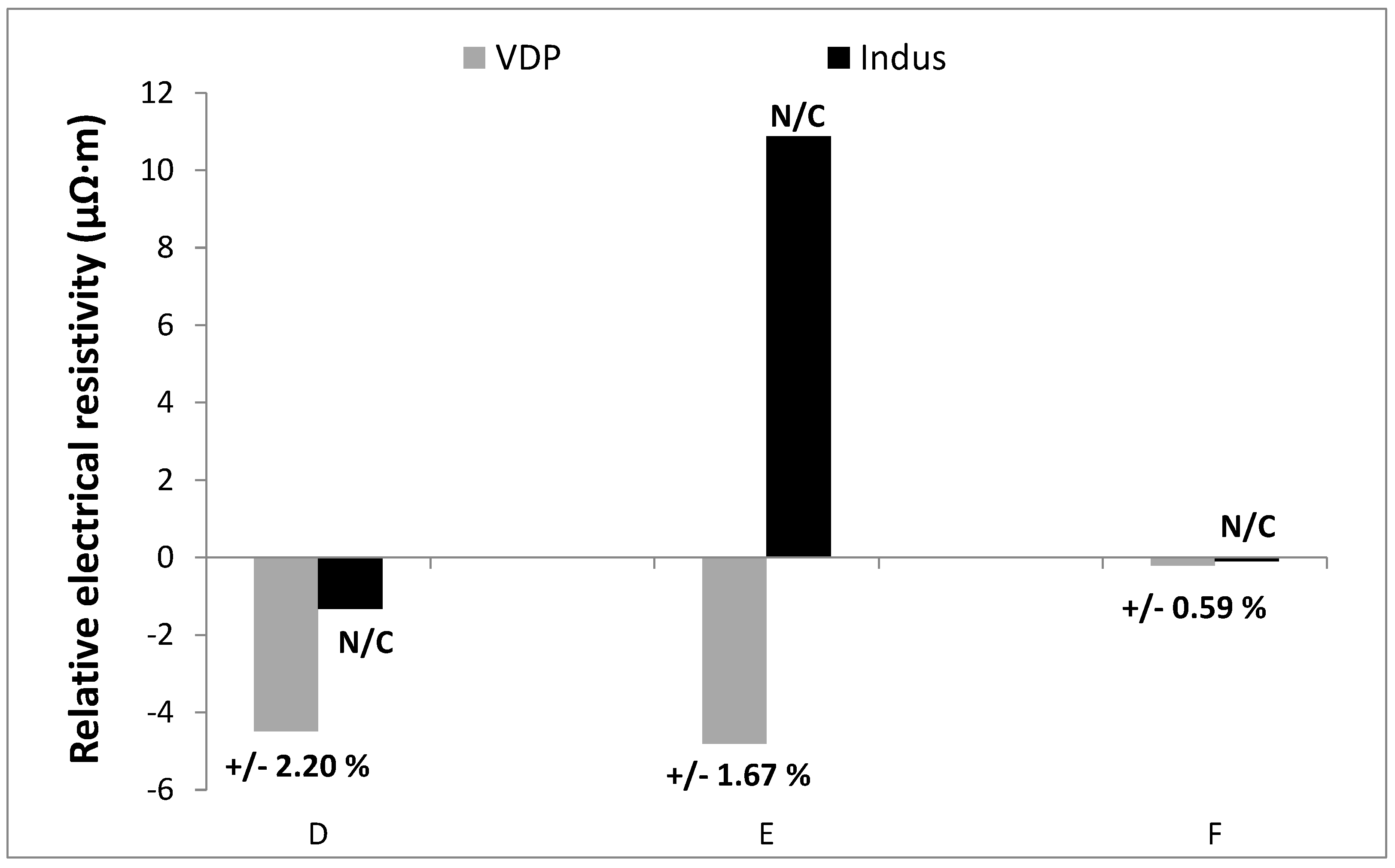
Figure 9.
Position of the crack toward the probes: (1) crack placed between two probes at equal distance; (2) crack placed close to one of the probes.
Figure 9.
Position of the crack toward the probes: (1) crack placed between two probes at equal distance; (2) crack placed close to one of the probes.

Figure 10.
CAD (Computer-Aaided Design) model used for the finite element method (FEM) and the VdP method, (A) radial crack, placed between the probes; (B) transverse crack.
Figure 10.
CAD (Computer-Aaided Design) model used for the finite element method (FEM) and the VdP method, (A) radial crack, placed between the probes; (B) transverse crack.

Figure 11.
Mesh model used for FEM and VdP methods; (A) radial crack, placed between the probes; (B) transverse cracks.
Figure 11.
Mesh model used for FEM and VdP methods; (A) radial crack, placed between the probes; (B) transverse cracks.
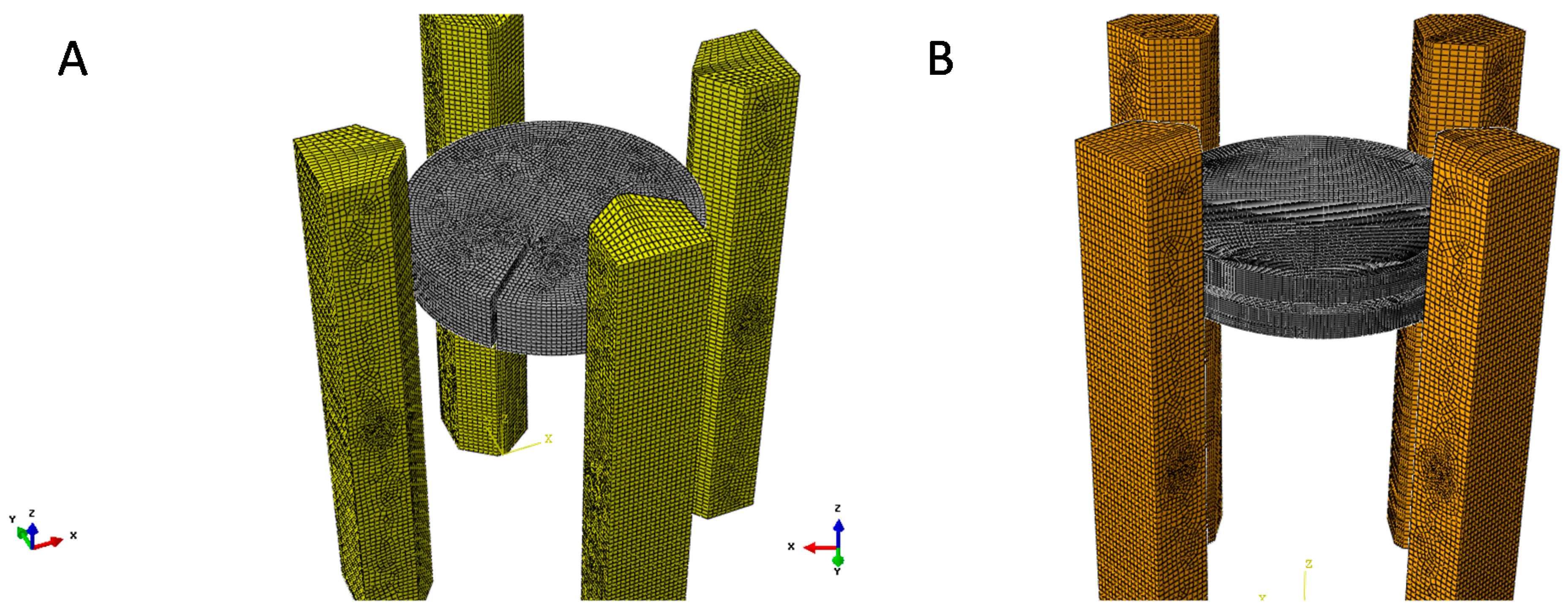
Figure 12.
Representation of the current line on a sample containing radial crack; (A) probes placed on the same side of the crack; (B) probes placed on both sides of the crack.
Figure 12.
Representation of the current line on a sample containing radial crack; (A) probes placed on the same side of the crack; (B) probes placed on both sides of the crack.


Table 1.
Electrical resistivity measurement of samples containing defects using both the standard and the Van der Pauw methods.
Table 1.
Electrical resistivity measurement of samples containing defects using both the standard and the Van der Pauw methods.
| Sample and Configuration | Relative Electrical Resistivity (μΩ∙m) |
|---|---|
| Measurements Using Standard Method | |
| Sample without defect | −2.4 ± 12% |
| Radial Crack | +5 ± 12% |
| void: 1.7% | |
| Transversal crack | +12.9 ± 21% |
| void: 0.18% | |
| Measurements using Van der Pauw method | |
| Sample without defect | +2.5 ± 0.4% |
| Radial Crack | +3.2 ± 2.5% |
| Crack placed between two probes | |
| Radial Crack | +3.3 ± 2% |
| Crack placed near the probe | |
| Transverse crack | +4.5 ± 8% |
Table 2.
Electrical resistivity estimation, using the FEM and VdP methods, for a sample containing a crack parallel to the axis of revolution.
Table 2.
Electrical resistivity estimation, using the FEM and VdP methods, for a sample containing a crack parallel to the axis of revolution.
| Crack Type and Position | Original Conductivity (S/m) | Electrical Conductivity Estimated Using FEM and VdP Methods (S/m) | Error |
|---|---|---|---|
| 2-mm wide crack, parallel to the axis of revolution, equal distance to sensors | 20,000 | 20,316 | +1.58% |
| 2-mm wide crack, parallel to the axis of revolution, close to one sensor | 20,000 | 20,260 | +1.30% |
| 0.1-mm thin crack, parallel to the axis of revolution, close to one sensor | 20,000 | 20,253 | +1.37% |
Table 3.
Electrical resistivity of a sample containing a crack, normal to the axis of rotation, calculated using the FEM and VdP methods.
Table 3.
Electrical resistivity of a sample containing a crack, normal to the axis of rotation, calculated using the FEM and VdP methods.
| Crack Type and Position | Original Conductivity (S/m) | Electrical Conductivity Estimated Using FEM and VdP Methods (S/m) | Error |
|---|---|---|---|
| 2-mm wide crack, normal to the axis of revolution | 20,000 | 19,362 | 3.19% |
| 0.1-mm thin crack, normal to the axis of revolution | 20,000 | 20,215 | +1.07% |
Table 4.
Difference for two contiguous resistances for a sample containing a crack parallel to the axis of rotation, calculated using the FEM method.
Table 4.
Difference for two contiguous resistances for a sample containing a crack parallel to the axis of rotation, calculated using the FEM method.
| Crack Type and Position | Original Conductivity (S/m) | Electrical Resistance Measured Using Finite Element Method | Difference |
|---|---|---|---|
| 2-mm wide crack, parallel to the axis of revolution, equal distance to sensors | 20,000 | R1 = 0.7 mΩ | 59.8% |
| R2 = 1.74 mΩ | |||
| 2-mm wide crack, parallel to the axis of revolution, close to one sensor | 20,000 | R1 = 0.52 mΩ | 73.9% |
| R2 = 1.99 mΩ | |||
| 0.1-mm thin crack, parallel to the axis of revolution, close to one sensor | 20,000 | R1 = 0.553 mΩ | 71.5% |
| R2 = 1.91 mΩ |
Table 5.
Difference for two contiguous resistances for a sample containing a crack normal to the axis of rotation, calculated using the FEM method.
Table 5.
Difference for two contiguous resistances for a sample containing a crack normal to the axis of rotation, calculated using the FEM method.
| Crack Type and Position | Original Conductivity (S/m) | Electrical Resistance Measured Using Finite Element Method | Difference |
|---|---|---|---|
| 2 mm wide crack, normal to the axis of revolution | 20,000 | R1 = 1.1 mΩ | 6.8% |
| R2 = 1.18 mΩ | |||
| 0.1 mm thin crack, normal to the axis of revolution | 20,000 | R1 = 1.086 mΩ | 0.99% |
| R2 = 1.0969 mΩ |
© 2017 by the authors. Licensee MDPI, Basel, Switzerland. This article is an open access article distributed under the terms and conditions of the Creative Commons Attribution (CC BY) license (http://creativecommons.org/licenses/by/4.0/).
Share and Cite
MDPI and ACS Style
Rouget, G.; Chaouki, H.; Picard, D.; Ziegler, D.; Alamdari, H. Electrical Resistivity Measurement of Carbon Anodes Using the Van der Pauw Method. Metals 2017, 7, 369. https://doi.org/10.3390/met7090369
AMA Style
Rouget G, Chaouki H, Picard D, Ziegler D, Alamdari H. Electrical Resistivity Measurement of Carbon Anodes Using the Van der Pauw Method. Metals. 2017; 7(9):369. https://doi.org/10.3390/met7090369
Chicago/Turabian StyleRouget, Geoffroy, Hicham Chaouki, Donald Picard, Donald Ziegler, and Houshang Alamdari. 2017. "Electrical Resistivity Measurement of Carbon Anodes Using the Van der Pauw Method" Metals 7, no. 9: 369. https://doi.org/10.3390/met7090369
Note that from the first issue of 2016, this journal uses article numbers instead of page numbers. See further details here.